the Correct Model?
Model Selection and Averaging of Impulse Responses*
Michael Pollmann†
Abstract
Impulse responses can be estimated to analyze the effects of a shock to a variable over time. Typically, (vector) autoregressive models are estimated and the impulse responses implied by the coefficients calculated. In general, however, there is no knowledge of the correct autoregressive order. In fact, when models are seen as approximations to the data generating process (DGP), all models are imperfect and there is no a priori difference in their validity. Hence, a lag length should be chosen by a sensible method, for instance an information criterion.
In Monte Carlo simulations, this paper studies what characteristics influence the optimal autoregressive order when all models are only approximations to the DGP. It finds that the precise coefficients in the DGP, the sample size, and the impulse response horizon to be estimated all influence the mean squared error-minimizing lag length. Furthermore, it evaluates the performance of model selection and averaging methods for estimating impulse responses. Across the characteristics found to be relevant, averaging outperforms model selection, and in particular Mallows’ Model Averaging and a smoothed Hannan-Quinn Information Criterion perform best. Finally, the study is extended to vector autoregressive models. In addition to the characteristics relevant in the univariate case, the optimal lag length also depends on which (cross) impulse response is to be estimated. Many issues remain for vector autoregressive models, however, and more work is necessary.
1 Introduction
The study of impulse response functions is of importance to many areas, for instance within
macroeconomics. Governments and central banks might attempt to predict the effects of
* Changes have been made for this publication. The original thesis is available from the author upon request. †
Michael Pollmann received a bachelor degree in Econometrics & Operations Research at Maastricht University in 2014, where he currently takes the Master in the same field. In fall 2015, he starts his Ph.D. in Economics at Stanford University.
their policies on the economy. For this purpose, vector autoregressive models are oftentimes
estimated to analyze the dynamics behind the underlying economic variables. To understand
the effect that a shock to one variable has over time on the system of variables studied, impulse response functions can be estimated. Unfortunately, however, many issues remain in this
estimation.
This paper focuses on what order of an autoregressive model should be chosen to minimize the mean squared error of the resulting estimator for the impulse response. Furthermore, it
compares the performance of various model selection and averaging techniques for estimating
impulse responses in a Monte Carlo study. Lastly, it offers preliminary insights into the study of these issues for vector autoregressive models.
In a brief paper, Hansen (2005) discusses challenges to model selection, focusing as an
example on the model also used in this paper. He criticizes the common assumption that the true data generating process is among the candidate models for model selection, and advocates the
use of selection methods specific to the purpose of the selected model. The Focused Information Criterion (FIC), developed by Claeskens and Hjort (2003), is such a method, asymptotically
selecting the model that minimizes the mean squared error of the estimator for the parameter of
interest. Claeskens et al. (2007) justify and demonstrate its use in the setting of this paper. When no candidate model is the true DGP, however, selecting one such model that is
known to be incorrect might be prone to a form of overfitting. As an alternative, estimates
of different models can be pooled and averaged based on a prespecified rule, for instance using smoothed information criteria. Claeskens and Hjort (2008) provide a detailed theoretical
treatment of information criteria (IC), in particular the FIC, and smoothed IC. In a simulation
study of forecasting quality, Hansen (2008) evaluates further averaging techniques.
The remainder of this paper is structured as follows. Section 2 presents some theoretical
background on the time series models used and the calculation of the impulse response functions.
Sections 3 and 4, respectively, offer an overview of the model selection and the averaging criteria employed. In section 5, the results of the Monte Carlo study are presented and their implications
discussed. Section 6 concludes.
2 The Model
This section presents the models considered in this paper. While the true DGP in all simulations
is a (vector) autoregressive moving-average model (ARMA), all candidate models are finite order (vector) autoregressive (AR) models. Section 2 provides theory for ARMA models, while
section 2 extends this to the VAR setting. Section 2 explains the use of the impulse response
ARMA(1,1)
The dynamics of an ARMA process depend solely on past values of the variable and shocks,
the autoregressive and moving-average parts, respectively. In general, an ARMA(p, q)model for the variableycan be written in terms of two polynomials,1
1−
p X
i=1
αiLi !
yt= 1− q X
i=1
βiLi !
t,
whereLidenotes the lag operator applieditimes, andt∼ N(0,1)in this paper. When the roots of the polynomial 1−Pp
i=1αiLi
lie outside the unit circle, the process is said to be stationary,
andytcan be written as an infinite sum of the present and past shockswith diminishing effects over time. Similarly, if the roots of the polynomial 1−Pq
i=1βiLi
lie outside the unit circle, the process is invertible. One can then writeytas an infinite sum of previous values ofyplus the present shock, t. An invertible ARMA process is therefore equivalent to an infinite order AR process.
In this paper, only ARMA(1,1) processes are used as DGP. Such a process takes the form
(1−αL)yt= (1−βL)t or, equivalently,
yt=αyt−1+t−βt−1 (2.1)
with the further restriction that the process is stationary and invertible, that is|α|< 1 and
|β|<1. As mentioned above, invertibility implies that an equivalent AR(∞)process exists. A special case arises whenα=β, and the ARMA(1,1) is white noise, that isyt=twith no time interdependencies; see appendix A for details.
In the simulations in this paper, models foryare estimated by AR(p) for finitep, of the structure
yt= p X
i=1
γiyt−i+t.
Hence, whenα6=βand thereforey is an AR(∞)process, none of the candidate models is the true DGP. This is a deliberate choice to put the econometrician in the usual situation where
all available models are only approximations to the DGP. As some properties of selection and
averaging methods depend on the true model being among the candidate models, this is a
1
situation of interest. In practice, one would likely try to consider (partial) autocorrelation functions
to determine lag orders for AR and MA polynomials. In the vector autoregressive models that
are the ultimate interest of this work, however, such strategies fail (Verbeek, 2012, ch. 9).
Vector Autoregressive Models
Vector autoregressive models (VAR) allow the dynamics of several variables to be modeled
together, taking into account interdependencies. They can be seen as reduced forms of
simultaneous equation models and therefore do not need additional restrictions to deal with identification issues. The reduced importance of a (potentially flawed) theoretical foundation
has been both praised and criticized. In macroeconomics, VARs have replaced many structural
equation models of the 1950s and 1960s and improved forecasting quality with small-scale models Greene (2007, ch. 20.6).
The general VAR(p)is similar to the univariate AR(p). Using vector notation, write
yt= p X
i=1
Γiyt−i+ut. (2.2)
For simplicity, only bivariate VARs are considered in this paper; that is, the system can be
written as
y1,t y2,t = p X i=1
γ11,i γ21,i γ12,i γ22,i
y1,t−i y2,t−i
+
u1,t u2,t
.
As this corresponds to seemingly unrelated regressions where each equation contains the
same set of explanatory variables, VAR can be estimated consistently and efficiently
equation-by-equation using OLS.
Any VAR(p)can be written as a VAR(1) using the companion matrix. For instance, instead of a bivariate VAR(2) in the form of equation 2.2, write
y1,t y2,t y1,t−1
y2,t−1
=
Γ1 Γ2
I 0
y1,t−1
y2,t−1
y1,t−2
y2,t−2
+
u1,t u2,t
whereIand0are the 2x2 identity and zero matrix, respectively. The companion matrix is then
Γ =
Γ1 Γ2
I 0
.
In this notation, the first two equations correspond to the original VAR(2), while the last two equations are identities. Technically, however, it is a VAR(1) with four variables. In shorter vector
notation,
zt= Γzt−1+vt (2.4)
with the obvious definitions ofzandv.
Such VARs will be used for estimation. The logical extension of the ARMA(1,1) that is the DGP in the setting of section 2 is the vector ARMA(1,1) (VARMA). Using lag polynomials,
(I−AL)yt= (I−BL)ut (2.5) for 2x2 matricesAandB, for which eigenvalues have moduli less than 1 to guarantee stability and invertibility Lütkepohl (2007, ch. 2 and 11), andut∼ N(0,I).
Impulse Responses
The impulse response function gives the effect that a unit-sized shock has on the dependent variable over time. In particular, when the process is written as
yt=t+θ1t−1+θ2t−2+θ3t−3+. . . (2.6)
then the impulse response at horizonhis given byθh. For example, figure 1 shows the impulse response function of the ARMA(1,1) processyt=−0.3yt−1+t−0.5t−1. For illustration,0 = 1
andt= 0for allt6= 0. By plugging these values into the formula,y0,y1,. . . can be calculated
iteratively and are equal to the values of the impulse response function at the corresponding
horizons.
From equation 2.1 one can calculate the impulse response function for general ARMA(1,1)
processes. Appendix A derives a general formula for the impulse response at horizonhas
θh= (α−β)αh−1. (2.7)
Figure 1– Example impulse response function for an ARMA(1,1) process,yt =−0.3yt−1+εt−
0.5εt−1. Here,ε0= 1andεt= 0∀t6= 0. The impulse response function gives the effect
of a unit shock on the dependent variable at different horizons.
expression. If, however, the AR(p)is written as a VAR(1), matrix algebra suffices. First, note that
yt= p X
i=1
γiyt−i+t
⇐⇒ yt yt−1
yt−2
.. .
yt−p−1
=
γ1 γ2 γ3 . . . γp
1 0 0 · · · 0
0 1 0 . . . 0
..
. ... ... . .. ...
0 0 0 . . . 0
yt−1
yt−2
yt−3
.. .
yt−p + t 0 0 .. . 0
with symbols properly defined.2 Recall that for an AR(1) processy
t=αyt−1+t, the impulse response at horizonhis simplyαh, the autoregressive coefficient to the power of the horizon.3 Intuitively, the same holds true for a VAR(1) process. Raising the coefficient matrix to the power ofh,Γh, and taking the coefficient ofyt−1in the equation foryt– that is, the element at position (1,1) ofΓh– gives the impulse response ofytat horizonh. Appendix A shows how this extends to the impulse responses of a VAR and offers a more formal mathematical derivation.
An alternative to analytical solutions for the impulse responses is based on simulations. With
the (estimated) coefficients, it is simple to set for instanceu1,t= 1and all other errorsu= 0to make recursive forecasts fory1,t+h, etc. (Canova, 2007, ch. 4). While possibly less elegant, this is a high-performance alternative especially to the inversion of the lag polynomial in equation 2.5
to find the impulse response of a VARMA process.
This is the simple case for VARs considered in this paper. Oftentimes, however, one finds the errors of the VAR to be contemporaneously correlated, that isVar [ut] = Σ6=σ2Iin equation 2.2. In that case, interest is usually not in shocks to the error terms in the VAR but instead to those of a structural VAR. Intuitively, if the error terms of the equations are not independent, one
is unlikely to observe a pure shock to only one variable as shocks for several variables usually
occur together.
General practice is to orthogonalize the errors, for instance through a Cholesky decomposition.
Such methods, however, are not unique, sometimes responsive to the ordering of the variables,
and in general different methods lead to different conclusions (Lütkepohl, 2007, ch. 2). Such issues and their interplay with model selection and averaging are not covered in this paper and
need to be studied in follow-up work.
3 Model Selection
Since the correct model is typically unknown, various techniques have been developed to select
a model from a set of candidate models. To evaluate several models, the value of an information
criterion can be computed for each. The econometrician then chooses the model with the best (typically lowest) IC. A range of IC has been developed, and most include a measure of fit based
on a likelihood function and a penalty for the number of explanatory variables used, even though the theoretical background might differ widely.
This paper considers Akaike’s Information Criterion (AIC), the Bayesian (also called Schwarz)
Information Criterion (BIC), and Hannan-Quinn Information Criterion (HQIC) of this structure.
2 In this context,Γis also called the companion matrix. 3
Another criterion, the Focused Information Criterion (FIC) by Claeskens and Hjort (2003) is
derived differently as an asymptotic estimate of the mean squared error of an estimator.
Akaike’s Information Criterion (Akaike, 1974) in the linear regression setting with normal errors of this paper can be calculated as
AIC =n·lnbσ2+ 2·p
for each model, wherenis the number of observations,bσ2 = RSSn (the residual sum of squares divided by n) the MLE for the variance, andp the AR order estimated (Claeskens and Hjort, 2008, ch. 2).4 One then selects the model with the lowest AIC. Here,
b
σ2 can be reduced by estimating a higher order AR model at the cost of increasingp. In its original formulation, the AIC estimates the loss of information in terms of the expected Kullback-Leibler distance between the estimated model and the unknown true model. Roughly speaking, choosing the model with
lowest AIC therefore asymptotically corresponds to choosing the model with a probability density
the most similar to that of the true data generating process (Claeskens and Hjort, 2008, ch. 2). A small sample correction can be based on the realization that the maximum likelihood
estimate bσ2 is consistent but biased. Burnham and Anderson (2004, ch. 6) advise to use such a correction in most situations based on better small sample performance and asymptotic equivalence. Burnham and Anderson (2004, ch. 7) derive this corrected AIC as
AICc=AIC+
2 (p+ 1) (p+ 2)
n−p−2 .
The Bayesian Information Criterion is originally based on Bayesian ideas Schwarz (1978). In
the Bayesian view, it is constructed to select the model with the highest posterior probability.
However, in practice one typically uses an approximation that removes the need to specify prior probabilities and strips the BIC of its Bayesian ideas (Claeskens and Hjort, 2008, ch. 3). In the
setting of this paper, it can then be calculated as
BIC =n·lnbσ2+p·lnn
and interpreted in the same way as the AIC. After calculating the BIC for all models, the model with the lowest BIC is chosen.
Some desirable properties of information criteria have been studied in the literature, but
are only stated here. Proofs, further explanations and details can be found in the referenced
4 Technically, this is not the AIC but only the terms that vary from model to model. Claeskens and Hjort (2008) report
papers. The AIC is efficient; that is, it asymptotically minimizes a loss function (Claeskens and
Hjort, 2008, ch. 4). The BIC asymptotically selects the true model if it is among the candidate
models (Burnham and Anderson, 2004, ch. 6), which is not satisfied in this paper. When the true model is not estimated, both the AIC and the BIC select a model that minimizes the
expected Kullback-Leibler distance to the true model. However, only the BIC will select the
smallest, or most parsimonious, of these “closest” models asymptotically, a property referred to as consistency (Claeskens and Hjort, 2008, ch. 4).
Roughly speaking, the AIC tries to find the best model taking into account the sample size and
therefore tends to choose larger models when the sample size increases. For consistency on the other hand, a criterion is expected to choose the correct model irrespective of the sample size;
that is, the criterion should choose the same model even as the sample size increases (Buckland
et al., 1997). To guarantee this, the penalty term needs to increase inn. Specifically, Sin and White (1996) show that one condition for strong consistency is that the penalty term must grow
at least as fast as ln lnnas the sample size increases. Clearly, the penalty term of the AIC, which is constant in the sample sizen, does not satisfy this, whereas the BIC does.
Another criterion, which was designed for strong consistency, the Hannan-Quinn Information
Criterion (Hannan and Quinn, 1979), was specifically developed in the context of order selection for autoregressive models. In the setting of this paper, it can be calculated as
HQIC =n·lnbσ2+ 2·p·ln lnn.
Interestingly, Hannan and Quinn (1979) originally multiply the penalty term by a constantc >1
to derive consistency of the criterion, and Claeskens and Hjort (2008, ch. 4) note that the choice of thiscis important for fine-tuning. However, Hannan and Quinn (1979) decide to usec= 1
“since it would seem pedantic, for the values ofN used [...], to choose some value ofcsuch as 1.01” (p. 194),5a choice that appears to have become standard practice and is followed in this paper.
In the context of lag length selection, AIC will select an AR order at least as large as HQIC,
which selects an order at least as large as BIC, for all but very small samples. Hence, neither HQIC nor AIC can possibly select fewer lags than BIC. Appendix A gives mathematical details.
Recalling that for stationary processes the impulse responses converge to 0, this allows a
hypothesis about the quality of criteria in the Monte Carlo study of this paper. Typically, a lower AR order implies that impulse responses are quicker to converge to 0. The relatively low AR
5 In the simulations of Hannan and Quinn (1979),
order chosen by the BIC might therefore be close in its estimation of the impulse response in
particular at large horizons, as then also the true impulse response is small in absolute value.
For large horizons, the BIC, and to a smaller extent also the HQIC, is therefore expected to perform relatively better.
A criterion based on a fundamentally different concept is the Focused Information
Crite-rion (Claeskens and Hjort, 2003). It is not based on a likelihood function, but instead an asymptotic estimate of the mean squared error in terms of bias and variance of a model with
respect to a particular parameter of interest. Hence, based on the same data, the FIC might
suggest a different model for estimating the impulse response at horizon 2 than for horizon 3. Due to its more complicated nature, no formula is presented here. A detailed description both
of theoretical derivations and practical implementations of the FIC in many different settings,
including linear regression, can be found in Claeskens and Hjort (2008, ch. 6).6 With its adjust-ment to the parameter of interest, the FIC takes a welcomed approach. Since its rather recent
development, relatively little is known of its performance. One could expect a good performance in the simulations of this paper, however, as criteria are evaluated based on the MSE of a
parameter of interest, which is minimized asymptotically by the FIC.
4 Model Averaging
An alternative to selecting an individual model is to average the estimates of several models. A
general framework for frequentist model averaging is developed by Hjort and Claeskens (2003).
Shen and Dougherty (2003) describe the choice between model selection and averaging as a choice between model interpretability and prediction quality. While the selection of a model
might be necessary to test for the significance of parameters or to understand the mechanism
behind a process, Shen and Dougherty (2003) recommend model averaging when prediction accuracy is the primary concern.
As an analogy to finance, buying a stock with good past performance might not be optimal.
Instead, a typical recommendation is to diversify risk by buying a portfolio of stocks. Model selection might similarly lead to a model that just by chance fits the sample very well, while
averaging yields better average performance by reducing the risk of this kind of overfitting. The hypotheses that averaging yields better performance and reduces the risk of large errors are
tested in the Monte Carlo study.
6
In its simplest form, averaging assigns equal weights (EW) to all models. For K models, where in this paperKis the maximum AR order plus 1 as an AR(0) model is estimated as well, each model receives weightwk = 1/K, fork= 1, . . . , K. The estimate for the impulse response that is of interest,θ, is then calculated from the estimated impulse responses of all models,θˆk, and the weights chosen by the averaging scheme,wk, as
ˆ
θ=
K X
i=1
wi·θˆi.
Hansen (2008) tests the performance of various averaging criteria for making one-step-ahead
forecasts in a simulation study. He finds that Mallow’s Model Averaging (MMA), smoothing based on AIC (sAIC), and the constrained Granger-Ramanathan weights perform best. In this paper, a
similar set of criteria is used for estimating impulse responses.
Hansen (2007) develops MMA and proves efficiency. Hansen (2008) extends the proof for stationary time series and shows that it asymptotically minimizes mean squared forecast errors.
MMA chooses weights to minimize the sum of residuals of the weighted models and a penalty based on the weighted number of parameters used, see Hansen (2007) for details.
Smoothing of information criteria has been proposed by Buckland et al. (1997). They suggest,
based on a Bayesian argument that assumes prior probabilities of the models to be equal, to give weightwk to each of theK models according to its information criterion value,ICk, as follows
wk=
exp (−ICk/2) PK
i=1exp (−ICi/2)
, k= 1, . . . , K.
This is an approximation of the Bayes factor (Buckland et al., 1997), and has the desirable
properties that two models with identical IC receive the same weight, a lower (better) IC results
in a higher weight, and weights sum to 1. In his study of forecasting quality, Hansen (2008) uses this to create the smoothed AIC (sAIC) and smoothed BIC (sBIC). For this paper, a similarly
constructed smoothed HQIC (sHQIC), of which no mention in the literature could be found so far,
is also used. Claeskens and Hjort (2008, ch. 10) propose slightly differently calculated weights for the smoothed FIC (sFIC), which are also used for the simulations in this paper.7
7 The constant
5 Results
This section presents results of Monte Carlo studies to evaluate the quality of model selection
and averaging techniques for estimating impulse responses. The general setup is the same for most studies. First, coefficient values α and β are chosen and the ARMA(1,1) process yt=αyt−1+t−βt−1is simulated. From the coefficients, the true impulse response can be
calculated. On each such sample, AR(p) forp = 0,1, . . . ,12, are estimated and the impulse response implied by the coefficients calculated. Furthermore, for each candidate AR(p), the models chosen by the selection criteria are determined. For averaging methods, the implied
impulse responses are averaged accordingly. Then, the squared errors of the estimated impulse responses are summed over all samples for each selection and averaging method, and the
result is reported as the mean squared error (MSE) of the estimator. For all simulations, 50,000
random samples are used.8
First, results are presented showing characteristics that influence the AR order that should be
chosen for estimating impulse responses. Second, the criteria of sections 3 and 4 are tested across these characteristics. Third, a brief study shows how the first results extend to vector
autoregressive models. On all these results, the following hypotheses are tested:
1. Averaging outperforms model selection. In particular, the risk of large errors is reduced.
2. Among the traditional information criteria; AIC, BIC, and HQIC; the criteria that tend to choose more parsimonious models will perform relatively better at large horizons. See
section 3 for an explanation.
3. Since the FIC can choose different models for different tasks, its performance is the most stable across IR horizons, while other criteria might be good for one horizon but perform
poorly on another.
4. The MSE of the criteria is lower for large samples than for small samples.
5. The characteristics that are relevant in the univariate case that is studied in detail in this paper are also relevant for vector autoregressive models.
Optimal AR order
For the first study, ARMA(1,1) processesyt=αyt−1+t−βt−1withαandβ ∈ {−0.9,−0.7, . . . ,0.9}
are simulated. For each of the 100 pairs of coefficients, samples of 200 effective observations are
8
Table 1– MSE-minimizing AR order for estimates of the impulse response at horizon 2 and 6 β
-0.9 -0.7 -0.5 -0.3 -0.1 0.1 0.3 0.5 0.7 0.9
-0.9 0/0 4/5 4/5 3/5 2/3 2/1 2/1 2/3 2/3 12/4
-0.7 8/2 0/0 4/3 2/2 2/1 1/2 1/3 4/3 2/3 2/1
-0.5 9/0 3/0 0/0 1/1 1/1 1/0 1/0 1/0 1/0 2/0
-0.3 8/0 3/0 0/0 0/0 1/0 1/0 2/0 3/0 4/0 1/0
α -0.1 0/0 0/0 0/0 0/0 0/0 0/0 0/0 0/0 0/0 4/0 0.1 4/0 0/0 0/0 0/0 0/0 0/0 0/0 0/0 0/0 0/0
0.3 1/0 4/0 3/0 2/0 1/0 1/0 0/0 0/0 3/0 10/0
0.5 2/0 1/0 1/0 1/0 1/0 1/1 1/2 0/0 3/0 11/0
0.7 2/1 2/3 2/3 1/3 1/1 2/1 2/2 4/3 0/0 10/2
0.9 11/4 2/4 2/1 2/1 2/1 2/2 2/4 3/5 4/5 0/0
The table can be read as follows: Whenα=−0.7andβ=−0.5, always selecting the AR(4) model resulted in a lower MSE for IR(2) than always selecting another AR(p)forp6= 4. Whenα= 0.5and β =−0.3, theoptimal AR order for IR(2) is 1. With the same parameter values, the optimal AR orders for estimating IR(6) are 3 and 0, respectively.
simulated. This is the same setting as in Hansen (2005). Table 1 shows for each parametrization
the AR order that minimizes MSE of the estimator for impulse responses at horizons 2 and 6.
The table closely resembles table 1 of Hansen (2005) and the conclusion remains the same. Since the optimal AR order depends on the coefficient values, which are typically unknown, a
selection or averaging technique is needed.
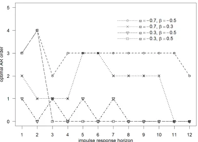
Furthermore, since the optimal AR order also depends on the impulse response horizon, it appears desirable to use a technique that can select a different AR orders to estimate the
impulse response for each horizon. For example, whenα=−0.7andβ =−0.5, the best AR order to estimate the IR at horizon 2 is 4, whereas at horizon 6 order 3 is best. Figure 2 gives further evidence. The optimal AR order is plotted on the vertical axis against the IR horizon on
the horizontal axis for different coefficient values. No clear relationship is apparent between IR horizon and optimal AR order. Only roughly and for relatively large IR horizons, the optimal AR
order appears to go down to 0.
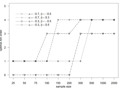
Lastly, the optimal AR order also depends on the sample size as figure 3 illustrates. The optimal AR order is plotted against sample sizes. Here, the number of effective observations for
Figure 2– The impulse response horizon is plotted against its MSE-minimizing AR order for different DGP. No clear relation is apparent. Lines are visual aids only.
number of observations, the optimal AR order increases.
Intuitively, this appears reasonable. When the number of observations increases, the increase in the variance of the coefficients when more explanatory variables are used becomes less
severe. Therefore, the variance of the implied impulse response, and thus also the MSE,
decreases when the sample size is increased. However, even with a sample size of 2,000 the optimal AR order is relatively low. Hence, in practical applications one cannot conclude that the
optimal AR order approaches the true AR(∞).
A notable exception to increasing optimal AR orders is the case ofα=β, not shown in figure 3, so the process is white noise. Then the true IR at any horizon (other than 0) is 0, which is exactly
the value implied by an AR(0). Whenα=β, the AR(0) is thus always the optimal model. Overall, one therefore needs to control for at least three characteristics when using AR models
to estimate impulse responses of ARMA(1,1) processes. First, different AR orders perform
best depending on the horizon at which one estimates the impulse response. This appears to be the most critical point. The FIC and sFIC are the only methods that take into account
Figure 3– Optimal AR order for IR horizon 2 depending on sample size for different coefficient values. In larger samples, MSE is minimized by higher AR orders. Lines are visual aids only; no sample sizes between points have been used for estimation.
independent of the IR horizon that is considered. It therefore appears reasonable expect a more
stable performance of the FIC. Second, great differences exist depending on the values ofα andβ. Typically, these values are unknown, so a criterion needs to perform well over at least a large region of coefficient values. Third, it is desirable to know how criteria perform depending
on sample size. This third problem, however, is the smallest. The sample size is known to the econometrician, so it is possible to use different criteria for small and large samples. Small
sample corrections as for the AICcmight improve the performance across sample sizes.
Performance of Criteria
In this section, results of a study of the performance of the model selection and averaging methods discussed in sections 3 and 4, respectively, along the dimensions investigated in
section 5 are discussed. Clearly, discussing results for all combinations of criteria, coefficient
paper therefore focuses almost exclusively on the mean squared error of the criteria to evaluate
performance, as it is also used by Hansen (2005) and Claeskens et al. (2007). The main text
proceeds with illustrative excerpts supporting the overall results, using graphical representations to allow different perspectives. References to the corresponding parts of the appendices, which
contain more numerical results, are given when appropriate.
First, the behavior of the criteria across coefficient values is studied. Table 2 shows the ratio of the MSE of AIC and FIC at impulse response horizon 2 with 200 effective observations and
50,000 simulations for each coefficient pair. Hansen (2005) creates a similar table for the ratio of
root MSE of FIC divided by AIC. However, neither values nor interpretation are compatible.9 In table 2, values below 1 imply that the average performance of the models selected by AIC
is better than that of the models selected by FIC for a given pair of coefficient values, whereas
ratios greater than 1 imply that FIC performed better. Here, AIC performs better along the “white noise diagonal” than FIC. On the first diagonal,α =β, so the true impulse response is 0. All coefficient pairs on the diagonal lead to the same white noise process, hence the ratios are almost equal. FIC appears to perform better than AIC when the moving average coefficient is
small in absolute value, and when both coefficients are large in absolute value but of opposite
sign.
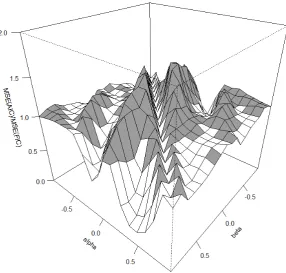
The table is visualized in the surface plot of figure 4. Axes and rotation are chosen to replicate
figure 3 of Claeskens et al. (2007) with the white noise diagonal in the center of the figure. The
resemblance is striking10and supports the conclusion that the ratios reported by Hansen (2005) are incorrect.
Ratio tables and surface plots can help to compare two criteria directly. To evaluate the
performance of all criteria, appendix B presents tables with individual MSE for impulse response horizon 2 with 200 effective observations and 50,000 simulations. Table 3 summarizes
infor-mation to compare inforinfor-mation criteria with weighting based on them. Clearly, the smoothed
IC outperform selecting an individual model, only for the (s)FIC this conclusion is less strong. The sIC lead to a lower MSE for almost all coefficient pairs as indicated by the first row. The
following rows compare the criteria and smoothed criteria on average MSE across coefficients
as well as maximal and minimal MSE. On all statistics, the sIC outperform model selection. In table 4, each column shows the MSE of criteria for one pair of coefficients as a summary
of appendix B. Since the sIC outperform the corresponding IC, these are skipped. The lowest
value in each column is marked with a star and implies that the criterion performed best for these coefficients. Overall, sBIC performs best when the DGP is white noise, but sHQIC, and
9 Footnote 6 also refers to this problem. 10
β
-0.9 -0.7 -0.5 -0.3 -0.1 0.1 0.3 0.5 0.7 0.9
-0.9 0.84 0.81 0.74 0.85 1.02 1.01 0.89 0.97 1.07 1.00
-0.7 0.57 0.85 0.89 0.95 1.00 1.02 1.05 0.99 1.01 1.04
-0.5 0.22 0.73 0.84 0.99 1.02 1.01 1.00 1.19 0.99 1.08
-0.3 0.42 0.45 1.05 0.84 1.18 1.10 0.96 0.77 0.80 1.03
α -0.1 0.95 1.28 1.28 1.45 0.86 1.56 1.29 1.05 0.83 0.52 0.1 0.56 0.86 1.07 1.35 1.55 0.85 1.45 1.27 1.21 0.91
0.3 1.10 0.82 0.80 0.96 1.12 1.16 0.86 1.05 0.46 0.45
0.5 1.09 1.02 1.23 1.02 1.01 1.02 0.98 0.85 0.71 0.22
0.7 1.04 1.02 1.00 1.04 1.01 1.00 0.93 0.90 0.86 0.55
0.9 1.00 1.07 0.98 0.90 1.00 1.03 0.91 0.82 0.79 0.85
Table 2– Ratio: MSE of AIC divided by MSE of FIC. Values below 1 imply better performance by AIC, values above 1 better performance by FIC.
AIC AICc BIC HQIC FIC
pct. sIC better 100 100 98 100 57
avg. MSE 8.53 8.52 9.53 8.73 9.69
avg. MSE sIC 8.10 8.06 8.64 8.02 8.22
max. MSE 24.68 24.73 27.03 25.31 29.66
max. MSE sIC 24.63 24.68 26.66 25.14 26.20
min. MSE 2.34 2.20 0.16 0.77 2.58
min. MSE sIC 2.10 1.95 0.13 0.67 3.78
Figure 4– Surface plot of table 2 including more coefficient pairs for a smoother figure. 5,000 simulations were run to calculate MSE. In the gray areas, the surface lies above 1 and AIC produces a higher (worse) MSE than FIC.
MMA show the best overall performance.
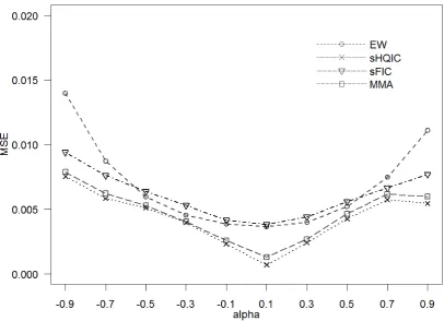
Figures 5 and 6 also help to compare the criteria. MSE is plotted againstαorβ, with the other coefficient held constant. A low line implies good performance. For graphical reasons, not all
criteria can be shown. Again, sHQIC and MMA show a constantly low MSE.
In a more realistic setting, the econometrician is unaware of the coefficient values and must choose a selection or weighting method without this information. Another Monte Carlo
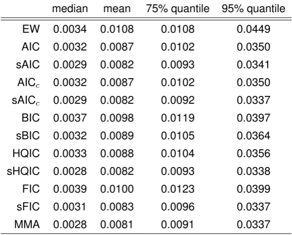
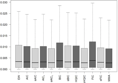
study allows comparing the performance of the criteria when in each simulation coefficients are independent draws from the uniform distribution,α, β ∼i.i.d. Uniform(−1,1). Figure 7 shows box plots of the squared errors of all criteria in the study. Table 5 summarizes this information. Again,
smoothed IC outperform selection based on IC. The difference in means is more pronounced than the difference in the medians. The last two columns offer a possible explanation: The
number of outliers, i.e. particularly large errors, is reduced significantly. Apparently smoothing
α, β
-0.7,-0.5 -0.7,0.3 -0.3,-0.5 -0.3,0.5 white noise
EW 4.28* 11.38 3.90* 6.57* 3.65
sAIC 5.38 9.87 5.20 8.53 2.13
sAICc 5.40 9.83 5.20 8.54 1.98
sBIC 7.01 9.31 6.03 9.57 0.14*
sHQIC 5.88 9.57 5.44 8.85 0.70
sFIC 5.28 9.70 4.76 8.25 3.82
MMA 5.50 9.29* 4.80 8.41 1.28
Table 4– MSE of criteria at IR horizon 2 for selected coefficient values, scaled up by a factor of 1,000. A star marks the best criterion in each column. Tables for all coefficient values can be found in appendix B.
Figure 6– MSE of criteria for fixedα= 0.5.
median mean 75% quantile 95% quantile
EW 0.0034 0.0108 0.0108 0.0449
AIC 0.0032 0.0087 0.0102 0.0350
sAIC 0.0029 0.0082 0.0093 0.0341
AICc 0.0032 0.0087 0.0102 0.0350
sAICc 0.0029 0.0082 0.0092 0.0337
BIC 0.0037 0.0098 0.0119 0.0397
sBIC 0.0032 0.0089 0.0105 0.0364
HQIC 0.0033 0.0088 0.0104 0.0356
sHQIC 0.0028 0.0082 0.0093 0.0338
FIC 0.0039 0.0100 0.0123 0.0399
sFIC 0.0031 0.0083 0.0096 0.0337
MMA 0.0028 0.0081 0.0091 0.0337
Figure 7– Box plot of squared errors of criteria for IR horizon 2 with 200 observations. The box covers the second and third quartile, the black line denotes the median. The whiskers do not extend to cover a fixed quantile but observations within a fixed multiple of the box interval length.
A similar analysis can be carried out for different IR horizons to evaluate the performance of criteria. Table 6 reproduces the earlier table 4 for IR horizon 6. Except for the second column,
MSE differ greatly. The complete overview in appendix B suggests that sHQIC and MMA still
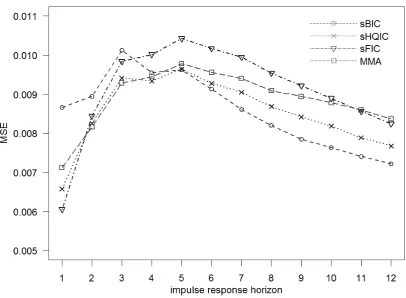
perform very well across all coefficient values, and sBIC also shows good performance. For an easier comparison of criteria across horizons, figure 8 returns to the study with random
coefficients. MSE are plotted against impulse response horizons. The good overall performance
of sHQIC is confirmed, but MMA shows relatively poor performance for large IR horizons. Furthermore, sBIC performs better for large IR horizons than for small horizons, affirming
hypothesis 2.
The figure also allows evaluating hypothesis 3 about FIC showing a more constant perfor-mance across horizons. This is not the case; the MSE of FIC varies as much across impulse
response horizons as the MSE of the other criteria. Apparently, selecting different models for
α, β
-0.7,-0.5 -0.7,0.3 -0.3,-0.5 -0.3,0.5 white noise
EW 1.87 9.12* 1.56 3.52 1.43
sAIC 1.50 10.80 0.97 4.62 0.55
sAICc 1.34 10.60 0.80 4.34 0.43
sBIC 0.86 9.83 0.02* 1.54* 0.00*
sHQIC 0.84* 9.78 0.15 2.66 0.04
sFIC 2.46 11.60 2.10 4.74 1.93
MMA 1.29 10.13 0.75 3.53 0.49
Table 6– MSE of criteria at IR horizon 6 for selected coefficient values, scaled up by a factor of 1,000. A star marks the best criterion in each column. Tables for all coefficient values can be found in appendix B
Figure 9– Comparison of AIC and AICcover sample sizes for IR horizon 2.
Figure 9 compares AIC and AICc, the small sample corrected version of the AIC. Again, the
coefficients in the simulations underlying the figure are drawn from the uniform distribution. The difference in performance for samples up to size 60 is another indication that size needs to
be considered. Choosing a sample size of 200 for the main results of the paper thus appears
justified for a first study to avoid small sample issues.
The scatterplot in figure 10 furthermore shows how the performance of all criteria improves in
larger samples, affirming hypothesis 4. Within each horizontal interval, the same sample size is
used, and the MSE for IR horizon 2 are plotted in the following order: AIC, BIC, sAIC, sBIC, EW, sFIC, AICc, sAICc, HQIC, sHQIC, FIC. In all but the very first interval, the second to last data
point, that is sHQIC, is among the lowest, confirming earlier results that it performs very well,
except for very small sample sizes.11
11The MMA is not shown in the plot due to numerical problems in its calculation for small samples that are rather
Figure 10– Scatterplot of MSE of criteria and sample sizes for IR horizon 2. Within each horizontal interval, the same sample size is used, and the MSE are plotted in the following order: AIC, BIC, sAIC, sBIC, EW, sFIC, AICc, sAICc, HQIC, sHQIC, FIC.
VAR
This section demonstrates that the preceding study and in particular the analysis of section 5 is
relevant for the estimation of impulse responses with vector autoregressive models. To achieve this, the optimal VAR order for estimating IR is found in Monte Carlo simulations. Rewriting
equation 2.5, the data generating process is
y1,t y2,t
=
0.7 −0.8 0.6 0.9
·
y1,t−1
y2,t−2
+
1,t 2,t
−
0.2 −0.6 0.4 −0.3
·
1,t−1
2,t−1
, (5.1)
with[1,t, 2,t]0∼ N(0,I)as in section 2. In each simulation, a sample allowing 200 effective observations for each estimated AR(p)is generated. For the DGP and each AR(p), the implied impulse response can be calculated as described in section 2 and appendix A.2 to calculate the
horizon
1 2 3 4 5 6
sample
siz
e
200 4 4
4 2 ! 4 2 2 4 ! 3 2 2 3 ! 2 4 1 3 ! 2 3 0 2 ! 1 3 2 3 !
50 2 2
2 2 ! 3 2 2 3 ! 2 2 2 0 ! 2 3 1 2 ! 2 0 0 2 ! 1 2 2 3 !
Table 7– The optimal AR orders for estimating the different impulse responses for sample sizes 50 and 200 at horizons 1 through 6, when the DGP is given by equation 5.1.
Θh =
θ11,h θ21,h θ12,h θ22,h
,
whereθ11,his the effect that a unit-sized shock toy1 has ony1 at horizonh. The effect of a
shock toy1 ony2 at horizonh isθ12,h, and θ21,h andθ22,h are defined likewise. Then table 7 shows in each cell a matrix with the optimal VAR orders for estimating the impulse responses
in the corresponding Θh. For instance, for a sample size of 200, it is optimal to use a VAR(4) to estimateθ11,1, but a VAR(2) is best for estimatingθ12,3. For a sample size of 50, a VAR(2) is
optimal for bothθ11,1 andθ12,3.
The table shows that the optimal AR order depends on the IR horizon to be estimated as the matrices within each row differ; hence different AR orders are optimal for different IR horizons.
Furthermore, also the sample size influences the optimal AR order as a comparison within each
column shows. Lastly, the optimal AR order depends on which (cross) impulse response is to be estimated. For fixedh, theθij,hvary withiandj. For instance, to study the effect at horizon 3 of a shock to variabley1ony2, a different AR order should be used than to study the effect of a
shock toy2 on itself.
To see whether also the coefficient values influence the optimal AR order, table 8 gives the
same overview but for the process
y1,t y2,t
=
0.4 −0.4 0.2 0.5
·
y1,t−1
y2,t−2
+ 1,t 2,t −
0.8 −0.1 0.5 −0.7
·
1,t−1
2,t−1
horizon
1 2 3 4 5 6
sample
siz
e
200 7 3
2 5 ! 0 2 2 1 ! 0 2 2 3 ! 2 3 0 0 ! 2 1 0 0 ! 0 0 0 0 !
50 4 3
2 4 ! 0 2 2 1 ! 0 2 0 0 ! 0 1 0 0 ! 0 1 0 0 ! 0 0 0 0 !
Table 8– The optimal AR orders for estimating the different impulse responses for sample sizes 50 and 200 at horizons 1 through 6, when the DGP is given by equation 5.2.
As expected, the optimal AR orders change from table 7 to table 8; that is, the coefficients of the DGP indeed influence the optimal AR orders.
To summarize, the same characteristics that are relevant in the univariate case are also
relevant for vector AR models, affirming hypothesis 5. Additionally, different AR orders are optimal for estimating the effects on different variables. Overall, an in-depth study similar to
section 5 is desirable.
6 Conclusion
This paper investigates the performance of various criteria for estimating impulse responses
when estimated models are only approximations to the true data generating process. The
optimal AR order for estimating IR depends on the coefficients chosen for the DGP, the IR horizon to be estimated, and the sample size. The same characteristics are also relevant for
vector autoregressive models. Furthermore, for VAR different lag lengths can be optimal for the different (cross) impulse responses of each variable.
In the univariate case, Mallows’ Model Averaging and in particular smoothing based on the
Hannan-Quinn information criterion perform best in the Monte Carlo simulations across the characteristics studied. Only for sample sizes below 50, smoothing of the AICcperforms better,
suggesting that a similar small sample correction to the Hannan-Quinn information criterion
could be considered. In general, averaging results in lower mean squared errors than selecting a single model; in particular, large errors are less common. The FIC and smoothed FIC, which are
the only criteria studied that adapt to the parameter estimated; that is, to the impulse response
The simulations in this paper only offer preliminary results for the vector autoregressive models
that are of greater practical importance. A more in-depth analysis is necessary to confirm that
the model characteristics found relevant here indeed translate directly to VARs, and performance of selection and averaging criteria is similar to AR models. Also, the effects of orthogonalization
of the errors need to be studied. Different orthogonalizations might be optimal depending on the
characteristics of the model and the model selection or averaging method used. Confidence intervals and bands for the estimates are of further interest. However, in VARs these pose
problems of their own, and Hjort and Claeskens (2003) and Claeskens and Hjort (2008, ch. 10)
discuss the additional difficulty as the model selection or averaging process needs to be taken into account.
References
Akaike, Hirotugu. (1974). A new look at the statistical model identification. Automatic Control,
IEEE Transactions on,19(6):716–723. doi:10.1109/TAC.1974.1100705.
Buckland, Steven T., Burnham, Kenneth P., & Augustin, Nicole H. (1997). Model Selection: An
Integral Part of Inference. Biometrics,53(2):603–618. doi:10.2307/2533961.
Burnham, Kenneth P., & Anderson, David R. (2004). Model Selection and Multimodel Inference:
A Practical Information-Theoretic Approach. Springer, New York, NY, second edition. ISBN 0387953647. doi:10.1007/b97636.
Canova, Fabio. (2007). Methods for Applied Macroeconomic Research. Princeton University
Press, Princeton, NJ. ISBN 0691115044. URLhttp://press.princeton.edu/titles/8434.
html.
Claeskens, Gerda, & Hjort, Nils Lid. (2003). The Focused Information Criterion. Journal of the American Statistical Association,98(464):900–916. doi:10.1198/016214503000000819.
Claeskens, Gerda, & Hjort, Nils Lid. (2008). Model Selection and Model Averaging. Cambridge
University Press, Cambridge, United Kingdom.
Claeskens, Gerda, Croux, Christophe, & Van Kerckhoven, Johan. (2007). Prediction focussed
model selection for autoregressive models. Australian & New Zealand Journal of Statistics,49
(4):359–379. doi:10.1111/j.1467-842X.2007.00487.x.
Hannan, Edward J., & Quinn, Brian G. (1979). The Determination of the Order of an
Autoregres-sion. Journal of the Royal Statistical Society. Series B (Methodological),41(2):190–195. ISSN
00359246. URLhttp://www.jstor.org/stable/2985032.
Hansen, Bruce E. (2005). Challenges for Econometric Model Selection. Econometric Theory,
21(1):60–68. doi:10.1017/S0266466605050048.
Hansen, Bruce E. (2007). Least Squares Model Averaging. Econometrica,75(4):1175–1189.
doi:10.1111/j.1468-0262.2007.00785.x.
Hansen, Bruce E. (2008). Least-squares forecast averaging. Journal of Econometrics,146(2):
342–350. doi:10.1016/j.jeconom.2008.08.022.
Hjort, Nils Lid, & Claeskens, Gerda. (2003). Frequentist Model Average Estimators. Journal of
the American Statistical Association,98(464):879–899. doi:10.1198/016214503000000828.
Hjort, Nils Lid, & Claeskens, Gerda. (2006). Focused Information Criteria and Model Averaging for the Cox Hazard Regression Model. Journal of the American Statistical Association,101
(476):1449–1464. doi:10.1198/016214506000000069.
Lütkepohl, Helmut. (2007). New Introduction to Multiple Time Series Analysis. Springer, Berlin,
Germany. ISBN 3540401725. doi:10.1007/978-3-540-27752-1.
Schwarz, Gideon. (1978). Estimating the Dimension of a Model. Annals of Statistics,6:461–464.
doi:10.1214/aos/1176344136.
Shen, Xiaotong, & Dougherty, Daniel P. (2003). Discussion: Inference and Interpretability Considerations in Frequentist Model Averaging and Selection. Journal of the American
Statistical Association,98(464):917–919. doi:10.1198/016214503000000837.
Sin, Chor-Yiu, & White, Halbert. (1996). Information criteria for selecting possibly
misspec-ified parametric models. Journal of Econometrics, 71(1-2):207–225. ISSN 0304-4076. doi:10.1016/0304-4076(94)01701-8.
Verbeek, Marno. (2012). A Guide to Modern Econometrics. Wiley, Chichester, United
King-dom, fourth edition. ISBN 1119951674. URL http://wiley.com/WileyCDA/WileyTitle/
Appendices
A Mathematics
White Noise Process
This appendix shows that the ARMA(1,1) process of equation 2.1 is a white noise process when
α=β. Let
yt=αyt−1+t−αt−1.
Rewrite this as
yt−t=α(yt−1−t−1),
and note that the equation holds for allt, in particular fort−h. Hence
yt−h−t−h=α(yt−h−1−t−h−1). (A.1)
Takingh= 1, substitute above to get
yt−t=α·a(yt−2−t−2).
Now, takeh= 2in equation A.1 and substitutea(yt−3−t−3)for(yt−2−t−2). By successive
substitution,
yt−t=αk·(yt−k−t−k)
fork= 1,2, . . . Taking the limit fork→ ∞and addingtto both sides,
=⇒ yt=t+ lim k→∞α
k·(y
t−k−t−k).
Since|a|<1,yis stationary, see section 2. Also sincet∼i.i.d. N(0,1), alsois stationary. Thus, with|a|<1,
lim
k→∞α k·(y
t−k−t−k) = 0 and henceyt=t; that is, the process is white noise.
Impulse Response of ARMA(1,1)
This appendix derives a general formula for the impulse response function of an ARMA(1,1)
time 0 onyh. Therefore, let0 = 1andt= 0for allt6= 0. Then by equation 2.1,
yh =αyh−1+h−βh−1.
In particular,y0=αy−1+0−β·−1. Since only06= 0,yh= 0for allh <0, and hencey0 = 1.
Then
y1=αy0+1−β0 =α·1 + 0−β·1.
Note thatyh, forh >1sumsh=h−1= 0as well asyh−1. Hence, forh >1,
yh=αyh−1 =αh−1y1 = (α−β)αh−1.
Since alsoy1 =α1−1(α−β), define for an ARMA(1,1) process in the form of equation 2.1 the
impulse response at horizonh≥1as
θh= (α−β)αh−1.
Impulse Response of VAR(p)
For a more formal derivation of the impulse response of an autoregressive process that also
includes the VARs discussed in section 2, first rewrite the VAR(p)as a VAR(1) as in equation 2.3, and then consider again equation 2.4. As before, the impulse response functions give the effect
of a unit-sized shock to one variable on the other variables.
In a bivariate VAR, there are hence four impulse responses at each horizon: the effect of a shock to variable 1 on variable 1, to variable 1 on variable 2, to variable 2 on variable 1, and
to variable 2 on variable 2. To calculate the response, for instance to a unit shock to the first
variabley1,0, setv0= (1,0,0,0)0. Then clearlyz0 = (1,0,0,0)0.
Since all further shocks are0, equation 2.4 implies thatz1 = Γz0+0,z2 = Γz1+0= Γ2z0
and in general
zh= Γhz0. (A.2)
Recalling the definition ofzh in equation 2.4,
zh = (y1,h, y2,h, y1,h−1, y2,h−1)0,
note that only the first two rows of Γhzt are relevant to find the effect ony1,h andy2,h. Since
z0= (1,0,0,0)0, the impulse responses of the variables to a shock to the first variable are equal
second column in equation A.2.
In general, the impulse responses at horizonh of the firstkvariables can be found in the upper leftk-by-ksubmatrix ofΓh. The univariate AR is therefore simply a special case, where the impulse response can be found in the upper left 1-by-1 submatrix of the companion matrix
Γh; that is, the IR is the element (1,1).
Ranking of AR Order Chosen by Criteria
In the setting of this paper, the candidate models can be ordered by the number of lags included. Due to their similar structure, one can then find a fixed ordering of the information criteria by
the number of lags included. In particular, for sufficiently large samples, AIC will always select
at least as many lags as HQIC and BIC, and HQIC will select at least as many lags as BIC. Mathematically, the following statement will be shown to be true.
Suppose two models, an AR(p) and an AR(q), are compared, whereq > p. Assume that BICq< BICp; that is, BIC selects the AR(q). Then∃N such that∀n > N,AICq < AICp; that is, AIC also selects the larger AR(q), wherenis the effective sample size.
By assumptionBICq−BICp <0. Using the formulas of section 3, rewrite this inequality as
nlnσb2q−nlnσbp2+qlnn−plnn <0.
Note thatAICq−AICp =nlnbσ
2
q −nlnbσ
2
p + 2q−2p. Clearly, the first two terms are the same as in the inequality of the BIC. Hence, if
2q−2p < qlnn−plnn,
thenAICq−AICp < BICq−BICp <0, so alsoAICq < AICp. Clearly,
2 (q−p)<lnn(q−p)
⇐⇒ 2<lnn ⇐= n≥8.
So withN = 7,∀n > N,AICq < AICp asn∈N. Hence, forn≥8, AIC selects at least as many lags as BIC.
Similarly, one can compare AIC with HQIC and HQIC with BIC by considering the penalty terms. For the former,
So for samples with at least 16 effective observations, AIC selects a model at least as large
as HQIC. Lastly, when comparing HQIC to BIC,
2 ln lnn <lnn ⇐= n≥2,
hence for all samples, HQIC selects models at least as large as BIC. Overall, for samples of at least 16 effective observations, the order of BIC is less than or equal to the order of HQIC,
B MSE of all Criteria
Appendix B contains tables with the MSE of all criteria and coefficient pairs for different impulse
response horizons and sample sizes. Appendix B uses 200 effective observations to estimate the impulse response at horizon 2. Appendix B uses 200 effective observations to estimate the
impulse response at horizon 6.
Impulse Response Horizon 2
This appendix gives detailed numerical results. The mean squared errors of all criteria for all coefficient pairs at impulse response horizon 2 with 200 effective observations are given. 50,000
simulations were run for each pair of coefficients. All MSE are scaled up by a factor of 1,000
for improved readability. Each criterion is shown in its own table. For example, whenα = 0.7
andβ = 0.3, equal weights result in a mean squared error of5.73·10−3 = 0.00573. When the AIC is used instead, the MSE for the same coefficient pair is6.66·10−3 = 0.00666, hence equal weights performs better (has a lower MSE) than the AIC for these coefficients. Color-coded tables that allow an easy comparison of the performance of a criterion for a given coefficient
pair to the performance of the other criteria for that coefficient pair are available in digital Excel
format from the author upon request.
β
-0.9 -0.7 -0.5 -0.3 -0.1 0.1 0.3 0.5 0.7 0.9
α
-0.9 3.65 4.20 5.02 6.38 9.41 13.96 19.68 27.61 39.40 69.24
-0.7 4.96 3.63 4.28 5.43 6.81 8.72 11.38 15.14 20.76 35.36
-0.5 7.50 3.98 3.67 4.10 4.91 5.98 7.34 9.04 11.57 16.77
-0.3 8.59 5.08 3.90 3.66 4.01 4.54 5.38 6.57 7.90 9.45
-0.1 8.14 5.98 4.61 3.85 3.64 3.87 4.48 5.47 6.81 7.90
0.1 7.78 6.65 5.43 4.50 3.92 3.65 3.84 4.70 6.32 8.92
0.3 10.06 8.17 6.81 5.64 4.67 4.02 3.66 3.95 5.35 9.41
0.5 18.97 12.82 9.99 7.96 6.43 5.20 4.15 3.64 4.12 8.16
0.7 39.33 23.82 17.19 12.87 9.74 7.49 5.73 4.44 3.64 5.24
0.9 77.23 45.34 31.75 22.98 16.26 11.10 7.51 5.54 4.48 3.61
β
-0.9 -0.7 -0.5 -0.3 -0.1 0.1 0.3 0.5 0.7 0.9
α
-0.9 2.36 6.23 7.35 7.55 7.02 9.69 12.80 15.69 18.70 22.87
-0.7 7.16 2.35 6.56 6.48 6.21 7.01 10.40 12.94 15.41 18.90
-0.5 6.36 7.32 2.41 5.14 5.05 6.02 8.42 10.54 12.53 15.36
-0.3 7.18 6.32 6.97 2.39 3.84 5.15 7.36 8.81 10.32 12.57
-0.1 8.38 7.15 7.18 5.42 2.40 4.06 7.20 7.41 8.48 10.09
0.1 10.44 8.58 7.42 7.06 3.99 2.37 5.54 7.20 7.14 8.48
0.3 12.91 10.44 8.87 7.31 5.08 3.83 2.39 7.08 6.28 7.26
0.5 16.05 12.87 10.74 8.39 6.03 5.30 5.29 2.38 7.31 6.48
0.7 19.89 15.89 13.19 10.40 7.29 6.50 6.66 6.87 2.40 7.26
0.9 24.68 19.63 16.41 13.07 10.56 7.16 7.22 7.26 6.49 2.34
Table 10– MSE of AIC at impulse response horizon 2 with 200 observations.
β
-0.9 -0.7 -0.5 -0.3 -0.1 0.1 0.3 0.5 0.7 0.9
α
-0.9 2.13 5.80 6.56 6.37 6.25 8.52 12.36 15.47 18.60 22.77
-0.7 6.32 2.13 5.38 5.71 5.91 6.84 9.87 12.73 15.30 18.78
-0.5 6.28 5.83 2.15 4.34 4.73 5.82 7.97 10.30 12.46 15.22
-0.3 7.07 6.26 5.20 2.14 3.60 4.73 6.83 8.53 10.24 12.44
-0.1 8.27 7.04 6.64 4.15 2.14 3.55 6.03 7.22 8.39 9.98
0.1 10.32 8.49 7.23 5.92 3.50 2.14 4.24 6.66 7.04 8.39
0.3 12.79 10.35 8.59 6.84 4.68 3.56 2.13 5.30 6.26 7.17
0.5 15.95 12.79 10.47 8.02 5.88 4.93 4.40 2.14 5.93 6.41
0.7 19.81 15.79 12.95 10.01 7.16 6.15 5.88 5.59 2.14 6.43
0.9 24.63 19.53 16.14 12.82 9.38 6.62 6.35 6.40 5.97 2.10
β
-0.9 -0.7 -0.5 -0.3 -0.1 0.1 0.3 0.5 0.7 0.9
α
-0.9 2.24 6.33 7.48 7.58 6.92 9.63 12.78 15.68 18.65 22.92
-0.7 7.45 2.23 6.64 6.50 6.16 6.91 10.38 12.94 15.36 18.88
-0.5 6.43 7.49 2.28 5.13 4.98 5.95 8.40 10.56 12.51 15.32
-0.3 7.20 6.35 7.08 2.27 3.74 5.09 7.38 8.84 10.30 12.52
-0.1 8.36 7.15 7.28 5.40 2.26 3.98 7.28 7.44 8.47 10.06
0.1 10.40 8.56 7.43 7.11 3.90 2.24 5.53 7.31 7.15 8.49
0.3 12.85 10.39 8.88 7.30 5.01 3.74 2.25 7.18 6.33 7.31
0.5 16.00 12.82 10.75 8.35 5.94 5.25 5.27 2.26 7.50 6.57
0.7 19.89 15.82 13.17 10.35 7.19 6.45 6.69 6.97 2.26 7.61
0.9 24.73 19.58 16.37 13.02 10.54 7.05 7.20 7.34 6.59 2.20
Table 12– MSE of AICcat impulse response horizon 2 with 200 observations.
β
-0.9 -0.7 -0.5 -0.3 -0.1 0.1 0.3 0.5 0.7 0.9
α
-0.9 1.98 5.86 6.62 6.34 6.11 8.40 12.33 15.46 18.56 22.79
-0.7 6.50 1.98 5.40 5.69 5.83 6.73 9.83 12.72 15.26 18.76
-0.5 6.35 5.90 2.00 4.28 4.65 5.74 7.94 10.31 12.43 15.18
-0.3 7.08 6.30 5.20 1.99 3.48 4.65 6.82 8.54 10.22 12.40
-0.1 8.25 7.04 6.70 4.07 1.99 3.43 6.05 7.25 8.39 9.95
0.1 10.28 8.47 7.24 5.92 3.38 1.99 4.17 6.74 7.05 8.39
0.3 12.74 10.32 8.59 6.81 4.59 3.45 1.98 5.31 6.32 7.21
0.5 15.91 12.75 10.46 7.97 5.80 4.85 4.34 1.99 6.01 6.50
0.7 19.80 15.75 12.93 9.95 7.05 6.09 5.87 5.62 1.99 6.63
0.9 24.68 19.50 16.10 12.76 9.29 6.47 6.28 6.45 6.04 1.95
β
-0.9 -0.7 -0.5 -0.3 -0.1 0.1 0.3 0.5 0.7 0.9
α
-0.9 0.18 11.62 12.46 8.55 5.64 9.19 13.73 15.95 18.45 24.42
-0.7 19.36 0.17 9.23 7.78 5.53 5.12 10.19 13.83 15.14 18.99
-0.5 15.66 13.27 0.17 4.82 3.91 4.76 7.82 11.83 12.52 14.68
-0.3 9.60 13.19 8.57 0.17 1.99 3.90 8.86 10.24 10.78 11.80
-0.1 8.95 9.02 13.50 4.29 0.16 2.02 9.67 10.48 9.62 9.92
0.1 9.96 9.37 9.96 9.06 1.82 0.19 4.69 13.99 9.45 9.45
0.3 12.01 10.61 9.79 8.26 3.54 2.08 0.16 9.07 13.76 10.20
0.5 15.50 12.62 11.41 7.38 4.51 4.28 5.20 0.17 13.75 16.77
0.7 20.41 15.52 13.50 9.74 5.56 6.02 8.54 10.01 0.19 19.79
0.9 27.03 19.49 16.01 13.25 11.18 5.43 7.10 11.14 12.18 0.16
Table 14– MSE of BIC at impulse response horizon 2 with 200 observations.
β
-0.9 -0.7 -0.5 -0.3 -0.1 0.1 0.3 0.5 0.7 0.9
α
-0.9 0.14 9.18 9.85 7.14 5.03 7.24 13.03 15.38 18.32 24.06
-0.7 15.46 0.14 7.01 6.19 5.30 5.16 9.31 13.19 15.02 18.80
-0.5 13.76 9.78 0.14 4.04 3.65 4.68 7.34 11.07 12.39 14.57
-0.3 9.33 11.12 6.03 0.14 1.83 3.54 7.67 9.57 10.58 11.72
-0.1 8.74 8.75 10.47 2.95 0.14 1.56 7.40 9.64 9.33 9.79
0.1 9.83 9.07 9.18 6.82 1.38 0.15 3.27 10.96 9.16 9.24
0.3 11.92 10.39 9.17 7.14 3.22 1.89 0.13 6.43 11.65 9.98
0.5 15.39 12.48 10.70 7.00 4.49 3.97 4.38 0.14 10.14 14.67
0.7 20.18 15.37 12.88 9.12 5.59 5.73 6.78 7.72 0.15 15.85
0.9 26.66 19.33 15.47 13.05 9.17 5.03 6.16 8.86 9.57 0.13
β
-0.9 -0.7 -0.5 -0.3 -0.1 0.1 0.3 0.5 0.7 0.9
α
-0.9 0.82 8.17 9.47 7.94 6.04 9.32 12.81 15.80 18.45 23.25
-0.7 13.04 0.82 7.90 7.09 5.71 5.87 10.34 13.28 15.18 18.85
-0.5 8.03 10.53 0.81 4.94 4.38 5.28 8.22 11.03 12.41 15.05
-0.3 7.60 7.93 8.26 0.78 2.65 4.47 7.95 9.38 10.33 12.25
-0.1 8.38 7.52 9.52 5.09 0.83 2.90 8.46 8.34 8.70 9.91
0.1 10.16 8.66 8.12 8.13 2.76 0.81 5.34 9.69 7.62 8.64
0.3 12.54 10.31 9.22 7.66 4.26 2.68 0.79 8.54 8.10 7.92
0.5 15.80 12.64 11.01 7.95 5.14 4.70 5.19 0.81 10.66 8.37
0.7 19.99 15.60 13.33 10.01 6.22 6.09 7.50 8.44 0.84 13.22
0.9 25.31 19.43 16.26 12.67 10.73 5.99 7.03 8.89 8.62 0.77
Table 16– MSE of HQIC at impulse response horizon 2 with 200 observations.
β
-0.9 -0.7 -0.5 -0.3 -0.1 0.1 0.3 0.5 0.7 0.9
α
-0.9 0.70 6.93 7.68 6.36 5.23 7.54 12.34 15.42 18.39 23.03
-0.7 9.63 0.70 5.88 5.76 5.39 5.83 9.57 12.85 15.10 18.69
-0.5 7.73 7.29 0.69 3.91 4.01 5.11 7.65 10.55 12.33 14.94
-0.3 7.42 7.47 5.44 0.68 2.42 3.97 7.06 8.85 10.24 12.14
-0.1 8.24 7.35 7.93 3.39 0.70 2.31 6.49 7.93 8.57 9.81
0.1 10.06 8.51 7.75 6.16 2.19 0.70 3.60 8.12 7.49 8.50
0.3 12.44 10.22 8.73 6.82 3.79 2.42 0.68 5.69 7.64 7.73
0.5 15.70 12.56 10.50 7.51 5.05 4.26 4.08 0.69 7.50 8.09
0.7 19.84 15.53 12.87 9.50 6.19 5.73 6.10 6.31 0.70 9.90
0.9 25.14 19.35 15.84 12.53 8.88 5.45 5.92 7.21 7.20 0.67
β
-0.9 -0.7 -0.5 -0.3 -0.1 0.1 0.3 0.5 0.7 0.9
α
-0.9 2.81 7.66 9.89 8.84 6.86 9.58 14.39 16.12 17.45 22.84
-0.7 12.64 2.77 7.36 6.80 6.23 6.85 9.92 13.05 15.29 18.21
-0.5 28.77 10.01 2.86 5.19 4.96 5.97 8.46 8.87 12.63 14.28
-0.3 17.08 13.93 6.67 2.83 3.26 4.69 7.64 11.50 12.94 12.23
-0.1 8.79 5.57 5.61 3.75 2.79 2.61 5.57 7.09 10.28 19.37
0.1 18.72 10.02 6.95 5.21 2.58 2.81 3.81 5.68 5.91 9.32
0.3 11.74 12.71 11.12 7.59 4.53 3.30 2.80 6.73 13.71 16.26
0.5 14.69 12.58 8.71 8.25 5.95 5.23 5.38 2.79 10.27 29.66
0.7 19.21 15.59 13.22 10.02 7.18 6.50 7.14 7.66 2.79 13.20
0.9 24.68 18.34 16.68 14.56 10.57 6.96 7.94 8.88 8.24 2.76
Table 18– MSE of FIC at impulse response horizon 2 with 200 observations.
β
-0.9 -0.7 -0.5 -0.3 -0.1 0.1 0.3 0.5 0.7 0.9
α
-0.9 3.82 5.46 5.98 6.53 7.28 9.40 12.70 15.12 17.84 23.66
-0.7 6.13 3.81 5.28 5.70 6.44 7.62 9.70 12.53 14.80 18.45
-0.5 7.80 5.25 3.85 4.84 5.41 6.38 7.75 9.52 12.02 14.29
-0.3 6.54 5.42 4.76 3.84 4.44 5.30 6.64 8.25 9.62 11.15
-0.1 8.67 6.17 5.09 4.26 3.82 4.15 5.34 6.96 8.80 9.93
0.1 9.77 8.70 6.95 5.31 4.18 3.83 4.24 5.14 6.42 9.27
0.3 11.17 9.48 8.28 6.76 5.33 4.42 3.83 4.75 5.46 7.06
0.5 15.06 12.21 9.66 7.88 6.52 5.59 4.86 3.81 5.30 8.18
0.7 19.80 15.21 12.78 10.05 7.90 6.65 5.82 5.41 3.82 6.29
0.9 26.20 18.83 15.78 13.39 10.00 7.69 6.66 5.93 5.66 3.78
β
-0.9 -0.7 -0.5 -0.3 -0.1 0.1 0.3 0.5 0.7 0.9
α
-0.9 1.28 6.09 7.07 6.45 5.67 7.88 12.17 15.36 18.57 23.68
-0.7 6.54 1.28 5.50 5.97 5.78 6.22 9.29 12.42 15.01 18.82
-0.5 7.50 5.61 1.30 3.93 4.34 5.29 7.45 9.98 12.12 14.77
-0.3 7.79 6.72 4.80 1.28 2.66 4.05 6.58 8.41 10.03 11.95
-0.1 8.38 7.34 6.78 3.46 1.29 2.58 5.89 7.41 8.52 9.80
0.1 9.93 8.39 7.23 5.66 2.52 1.29 3.60 6.95 7.58 8.79
0.3 12.20 9.99 8.32 6.44 3.95 2.67 1.28 4.99 6.96 8.25
0.5 15.60 12.39 10.05 7.41 5.33 4.65 4.07 1.29 5.80 7.99
0.7 20.14 15.60 12.62 9.47 6.62 6.16 6.34 5.84 1.29 6.82
0.9 26.20 19.84 16.13 12.82 9.19 5.98 6.19 6.89 6.40 1.26
Table 20– MSE of MMA at impulse response horizon 2 with 200 observations.
Impulse Response Horizon 6
This appendix gives detailed numerical results. The mean squared errors of all criteria for all coefficient pairs at impulse response horizon 6 with 200 effective observations are given. 50,000
simulations were run for each pair of coefficients. All MSE are scaled up by a factor of 1,000
for improved readability. Each criterion is shown in its own table. For example, whenα = 0.7
andβ = 0.3, equal weights result in a mean squared error of3.04·10−3 = 0.00304. When the
AIC is used instead, the MSE for the same coefficient pair is3.13·10−3 = 0.00313, hence equal weights performs better (has a lower MSE) than the AIC for these coefficients. Color-coded
tables that allow an easy comparison of the performance of a criterion for a given coefficient
β
-0.9 -0.7 -0.5 -0.3 -0.1 0.1 0.3 0.5 0.7 0.9
α
-0.9 1.43 3.19 5.88 8.94 12.86 18.26 25.30 35.23 47.39 67.13
-0.7 2.23 1.42 1.87 2.84 4.35 6.51 9.12 12.23 15.89 19.19
-0.5 2.28 1.62 1.44 1.62 2.15 3.03 4.27 5.98 7.73 9.35
-0.3 2.47 1.94 1.56 1.44 1.57 1.95 2.61 3.52 4.64 5.74
-0.1 3.06 2.44 1.90 1.55 1.44 1.56 1.90 2.46 3.25 4.07
0.1 3.96 3.24 2.44 1.85 1.56 1.44 1.56 1.89 2.46 3.13
0.3 5.71 4.63 3.47 2.57 1.93 1.55 1.45 1.57 1.95 2.55
0.5 9.45 7.86 6.00 4.38 3.07 2.16 1.62 1.43 1.64 2.38
0.7 21.93 17.73 13.48 9.96 6.94 4.73 3.04 1.93 1.43 2.38
0.9 87.59 62.39 45.74 33.67 24.03 17.00 11.91 7.74 3.84 1.42
Table 21– MSE of equal weights at impulse response horizon 6 with 200 observations.
β
-0.9 -0.7 -0.5 -0.3 -0.1 0.1 0.3 0.5 0.7 0.9
α
-0.9 0.74 4.99 6.06 8.42 12.23 16.13 24.74 35.41 51.46 61.81
-0.7 5.12 0.66 1.96 3.11 4.07 7.11 11.69 17.14 23.50 28.66
-0.5 6.52 2.16 0.70 1.13 1.53 2.60 5.14 10.49 14.73 17.67
-0.3 7.13 3.83 1.33 0.70 1.02 1.38 2.61 5.88 11.00 12.67
-0.1 8.29 5.79 2.09 1.11 0.70 1.00 1.59 3.41 8.38 9.95
0.1 9.83 8.24 3.25 1.49 1.01 0.71 1.12 2.19 6.06 8.36
0.3 12.82 11.13 5.60 2.44 1.31 0.97 0.73 1.35 4.07 7.29
0.5 17.98 15.24 10.39 5.03 2.55 1.51 1.11 0.70 2.30 6.66
0.7 30.72 25.08 18.30 12.26 7.02 4.22 3.13 1.90 0.71 5.25
0.9 70.90 58.02 41.17 30.65 19.95 15.22 10.58 7.38 5.53 0.70
β
-0.9 -0.7 -0.5 -0.3 -0.1 0.1 0.3 0.5 0.7 0.9
α
-0.9 0.55 4.05 5.48 8.04 11.61 15.71 23.75 33.84 48.92 61.35
-0.7 3.78 0.50 1.50 2.56 3.64 6.37 10.80 16.17 22.56 28.34
-0.5 5.53 1.51 0.52 0.86 1.25 2.13 4.36 8.79 13.92 17.47
-0.3 6.59 2.84 0.97 0.53 0.77 1.08 2.07 4.62 9.66 12.53
-0.1 7.97 4.47 1.57 0.82 0.54 0.75 1.20 2.63 6.82 9.81
0.1 9.65 6.69 2.51 1.14 0.75 0.52 0.83 1.65 4.68 8.08
0.3 12.66 9.70 4.38 1.93 1.04 0.74 0.55 0.98 3.01 6.75
0.5 17.76 14.30 8.70 4.35 2.08 1.23 0.85 0.52 1.64 5.65
0.7 30.41 24.13 17.30 11.45 6.30 3.80 2.64 1.48 0.52 3.96
0.9 70.51 55.62 39.82 29.52 19.52 14.56 10.17 6.77 4.55 0.51
Table 23– MSE of sAIC at impulse response horizon 6 with 200 observations.
β
-0.9 -0.7 -0.5 -0.3 -0.1 0.1 0.3 0.5 0.7 0.9
α
-0.9 0.60 4.94 5.97 8.27 12.07 15.77 24.38 34.97 51.50 61.77
-0.7 5.00 0.53 1.78 2.94 3.87 6.91 11.50 17.03 23.46 28.62
-0.5 6.59 1.93 0.56 0.95 1.33 2.36 4.88 10.41 14.83 17.63
-0.3 7.22 3.62 1.13 0.58 0.84 1.17 2.35 5.68 11.11 12.68
-0.1 8.35 5.65 1.84 0.92 0.57 0.83 1.36 3.13 8.40 10.00
0.1 9.83 8.24 2.97 1.29 0.83 0.56 0.93 1.93 5.95 8.45
0.3 12.79 11.23 5.37 2.18 1.11 0.80 0.59 1.15 3.87 7.41
0.5 17.94 15.34 10.28 4.75 2.31 1.30 0.93 0.56 2.08 6.76
0.7 30.65 25.11 18.19 12.06 6.77 3.99 2.95 1.73 0.57 5.16
0.9 70.89 58.18 40.82 30.40 19.63 15.11 10.49 7.37 5.50 0.56
β
-0.9 -0.7 -0.5 -0.3 -0.1 0.1 0.3 0.5 0.7 0.9
α
-0.9 0.43 4.00 5.43 7.96 11.48 15.42 23.43 33.38 48.68 61.28
-0.7 3.64 0.39 1.34 2.41 3.44 6.15 10.60 16.02 22.44 28.27
-0.5 5.45 1.32 0.41 0.70 1.06 1.91 4.10 8.58 13.89 17.43
-0.3 6.55 2.61 0.80 0.41 0.62 0.90 1.82 4.34 9.59 12.52
-0.1 7.95 4.25 1.35 0.66 0.42 0.60 1.01 2.37 6.68 9.81
0.1 9.63 6.52 2.25 0.95 0.60 0.41 0.67 1.43 4.47 8.08
0.3 12.62 9.62 4.10 1.68 0.86 0.59 0.43 0.81 2.78 6.74
0.5 17.69 14.26 8.47 4.06 1.85 1.05 0.69 0.40 1.44 5.59
0.7 30.34 24.03 17.14 11.23 6.06 3.58 2.48 1.33 0.40 3.83
0.9 70.51 55.51 39.52 29.33 19.27 14.48 10.14 6.77 4.53 0.40
Table 25– MSE of sAICc at impulse response horizon 6 with 200 observations.
β
-0.9 -0.7 -0.5 -0.3 -0.1 0.1 0.3 0.5 0.7 0.9
α
-0.9 0.00 6.67 7.99 10.52 12.51 12.51 23.48 31.20 49.75 68.67
-0.7 1.54 0.00 1.00 2.48 2.42 5.39 11.19 19.06 23.30 29.71
-0.5 3.48 0.13 0.00 0.07 0.15 0.81 3.24 9.68 18.71 19.30
-0.3 6.68 0.68 0.03 0.00 0.01 0.04 0.45 2.59 12.96 15.98
-0.1 10.36 2.43 0.15 0.01 0.00 0.01 0.06 0.60 6.67 13.67
0.1 13.51 6.39 0.54 0.05 0.01 0.00 0.01 0.17 2.69 10.67
0.3 16.28 13.11 2.29 0.39 0.04 0.01 0.00 0.03 0.80 7.14
0.5 19.97 19.26 9.23 2.92 0.67 0.14 0.06 0.00 0.15 3.68
0.7 32.50 25.19 20.57 11.80 4.67 2.59 2.56 0.99 0.00 1.58
0.9 79.54 57.50 39.64 30.34 15.98 16.21 13.71 10.36 7.70 0.00