Two-Stage Performance Engineering of Container-based Virtualization

(1)

www.astesj.com

Special issue on Advancement in Engineering Technology

ISSN: 2415-6698

Two-Stage Performance Engineering of Container-based

Virtualization

Zheng Li1,4, Maria Kihl*,2, Yiqun Chen3, He Zhang1

1_{Software Institute, Nanjing University, 210008, China}

2_{Department of Electrical and Information Technology, Lund University, 223 63, Sweden}

3_{Centre for Spatial Data Infrastructures & Land Administration, University of Melbourne, 3010, Australia} 4_{Department of Computer Science, University of Concepci´on, 4070386, Chile}

A R T I C L E I N F O A B S T R A C T

Article history:

Received: 14 November, 2017 Accepted: 05 February, 2018 Online: 28 February, 2018 Keywords:

Cloud Computing Container Hypervisor MapReduce

Performance Engineering Virtualization

Cloud computing has become a compelling paradigm built on compute and storage virtualization technologies. The current virtualization solu-tion in the Cloud widely relies on hypervisor-based technologies. Given the recent booming of the container ecosystem, the container-based vir-tualization starts receiving more attention for being a promising alter-native. Although the container technologies are generally considered to be lightweight, no virtualization solution is ideally resource-free, and the corresponding performance overheads will lead to negative impacts on the quality of Cloud services. To facilitate understanding container technologies from the performance engineering’s perspective, we con-ducted two-stage performance investigations into Docker containers as a concrete example. At the first stage, we used a physical machine with “just-enough” resource as a baseline to investigate the performance overhead of a standalone Docker container against a standalone virtual machine (VM). With findings contrary to the related work, our evalua-tion results show that the virtualizaevalua-tion’s performance overhead could vary not only on a feature-by-feature basis but also on a job-to-job basis. Moreover, the hypervisor-based technology does not come with higher performance overhead in every case. For example, Docker containers par-ticularly exhibit lower QoS in terms of storage transaction speed. At the ongoing second stage, we employed a physical machine with “fair-enough” resource to implement a container-based MapReduce application and try to optimize its performance. In fact, this machine failed in aff ord-ing VM-based MapReduce clusters in the same scale. The performance tuning results show that the effects of different optimization strategies could largely be related to the data characteristics. For example, LZO compression can bring the most significant performance improvement when dealing with text data in our case.

1 Introduction

The container technologies have widely been accepted for building next-generation Cloud systems. This pa-per investigates the pa-performance overhead of container-based virtualization and the performance optimization of a container-based MapReduce application, which is an extension of work originally presented in the 31st

IEEE International Conference on Advanced Informa-tion Networking and ApplicaInforma-tion (AINA 2017) [1].

The Cloud has been considered to be able to pro-vide computing capacity as the next utility in our mod-ern daily life. In particular, it is the virtualization technologies that enable Cloud computing to be a new paradigm of utility, by playing various vital roles in supporting Cloud services, ranging from resource

iso-*_{Corresponding Author; Address: Ole R¨omers V¨ag 3, Lund 223 63, Sweden; Tel: + 46 46 222 9010; Email: [email protected]}

(2)

Z. Li et al. / Advances in Science, Technology and Engineering Systems Journal Vol. 3, No. 1, 521-536 (2018)

lation to resource provisioning. The existing virtu-alization technologies can roughly be distinguished between the hypervisor-based and the container-based solutions. Considering their own resource consump-tion, both virtualization solutions inevitably introduce performance overheads to running Cloud services, and the performance overheads could then lead to negative impacts to the corresponding quality of service (QoS). Therefore, it would be crucial for both Cloud providers (e.g., for improving infrastructural efficiency) and con-sumers (e.g., for selecting services wisely) to under-stand to what extend a candidate virtualization solu-tion incurs influence on the Cloud’s QoS.

Recall that hypervisor-driven virtual machines (VMs) require guest operating systems (OS), while con-tainers can share a host OS. Suppose physical machines, VMs and containers are three candidate resource types for a particular Cloud service, a natural hypothesis could be:

The physical machine-based service has the best quality among the three resource types, while the container-based service performs better than the hypervisor-based VM service.

Unfortunately, to the best of our knowledge, there is little quantitative evidence to help test this hypothe-sis in an “apple-to-apple” manner, except for the sim-ilar qualitative discussions. Furthermore, the perfor-mance overhead of hypervisor-based and container-based virtualization technologies can even vary in prac-tice depending on different service circumstance (e.g., uncertain workload densities and resource competi-tions). Therefore, we decided to conduct a twofold investigation into containers from the performance’s perspective. Firstly, we used a physical machine with “just-enough” resource as a baseline to quantitatively investigate and compare the performance overheads between the container-based and hypervisor-based vir-tualizations. In particular, since Docker is currently the most popular container solution [2] and VMWare is one of the leaders in the hypervisor market [3], we chose Docker and VMWare Workstation 12 Pro to rep-resent the two virtualization solutions respectively. Secondly, we implemented a container-based MapRe-duce cluster on a physical machine with “fair-enough” resource to investigate the performance optimization of our MapReduce application at least in this use case.

According to the clarifications in [4, 5], our qualita-tive investigations can be regulated by the discipline of experimental computer science (ECS). By employing ECS’s recently available Domain Knowledge-driven Methodology (DoKnowMe) [6], we experimentally ex-plored the performance overheads of different virtual-ization solutions on a feature-by-feature basis, i.e. the communication-, computation-, memory- and storage-related QoS aspects. As for the investigation into performance optimization, we were concerned with the task timeout, out-of-band heartbeat, buffer setting, stream merging, data compression and the cluster size of our container-based MapReduce application.

The experimental results and analyses of perfor-mance overhead investigation generally advocate the aforementioned hypothesis. However, the hypothe-sis is not true in all the cases. For example, we do not see computation performance difference between the three resource types for solving a combinatorially hard chess problem; and the container exhibits even higher storage performance overhead than the VM when reading/writing data byte by byte. Moreover, we find that the remarkable performance loss incurred by both virtualization solutions usually appears in the performance variability.

The performance optimization investigation re-veals that various optimization strategies might take different effects due to different data characteristics of a container-based MapReduce application. For ex-ample, dealing with text data can significantly benefit from enabling data compression, whereas buffer set-tings have little effect for dealing with relatively small amount of data.

Overall, our work makes fourfold contributions to the container ecosystem, as specified below.

(1) Our experimental results and analyses can help both researchers and practitioners to better un-derstand the fundamental performance of the present container-based and hypervisor-based virtualization technologies. In fact, the perfor-mance evaluation practices in ECS can roughly be distinguished between two stages: the first stage is to reveal the primary performance of spe-cific (system) features, while the second stage is generally based on the first-stage evaluation to investigate real-world application cases. Thus, this work can be viewed as a foundation for more sophisticated evaluation studies in the future.

(2) Our method of calculating performance over-head can easily be applied or adapted to diff er-ent evaluation scenarios by others. The literature shows that the “performance overhead” has nor-mally been used in the context of qualitative dis-cussions. By quantifying such an indicator, our study essentially provides a concrete lens into the case of performance comparisons.

(3) As a second-stage evaluation work, our case study on the performance optimization of a MapReduce application both demonstrates a practical use case and supplies an easy-to-replicate scenario for engineering performance of container-based applications. In other words, this work essentially proposed a characteristic-consistent data set (i.e. Amazon’s spot price his-tory that is open to the public) for future perfor-mance engineering studies.

(3)

can be conveniently repeated or replicated even by different evaluators at different times and locations. More importantly, by emphasizing the backend logic and evaluation activities, the template-driven evaluation implementations (in-stead of results only) would be more traceable and comparable.

The remainder of this paper is organized as follows. Section 2 briefly summarizes the background knowl-edge of container-based and the hypervisor-based vir-tualization technologies. Section 3 introduces the fundamental performance evaluation of a single con-tainer. The detailed performance overhead investi-gation is divided into two reporting parts, namely pre-experimental activities and experimental results & analyses, and they are correspondingly described into Section 3.2 and 3.3 respectively. Section 4 explains our case study on the performance optimization of a container-based MapReduce application. Section 5 highlights the existing work related to container’s per-formance evaluation. Conclusions and some future work are discussed in Section 6.

2 Hypervisor-based vs.

Container-based Virtualization

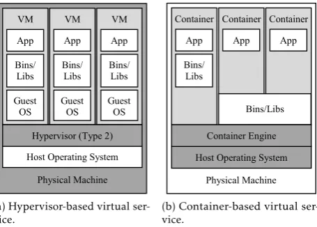
When it comes to the Cloud virtualization, the de facto solution is to employ the hypervisor-based technolo-gies, and the most representative Cloud service type is offering VMs [8]. In this virtualization solution, the hypervisor manages physical computing resources and makes isolated slices of hardware available for creat-ing VMs [7]. We can further distcreat-inguish between two types of hypervisors, namely the bare-metal hypervisor that is installed directly onto the computing hardware, and the hosted hypervisor that requires a host OS. To make a better contrast between the hypervisor-related and container-related concepts, we particularly empha-size the second hypervisor type, as shown in Figure 1a. Since the hypervisor-based virtualization provides access to physical hardware only, each VM needs a com-plete implementation of a guest OS including the bina-ries and librabina-ries necessary for applications [9]. As a result, the guest OS will inevitably incur resource com-petition against the applications running on the VM service, and essentially downgrade the QoS from the application’s perspective. Moreover, the performance overhead of the hypervisor would also be passed on to the corresponding Cloud services and lead to negative impacts on the QoS.

To relieve the performance overhead of hypervisor-based virtualization, researchers and practition-ers recently started promoting an alternative and lightweight solution, namely container-based virtual-ization. In fact, the foundation of the container technol-ogy can be traced back to the Unixchrootcommand in 1979 [9], while this technology is eventually evolved into virtualization mechanisms like Linux VServer, OpenVZ and Linux Containers (LXC) along with the

booming of Linux [10]. Unlike the hardware-level so-lution of hypervisors, containers realize virtualization at the OS level and utilize isolated slices of the host OS to shield their contained applications [9]. In essence, a container is composed of one or more lightweight images, and each image is a prebaked and replaceable file system that includes necessary binaries, libraries or middlewares for running the application. In the case of multiple images, the read-only supporting file systems are stacked on top of each other to cater for the writable top-layer file system [2]. With this mechanism, as shown in Figure 1b, containers enable applications to share the same OS and even binaries/libraries when appropriate. As such, compared to VMs, containers would be more resource efficient by excluding the exe-cution of hypervisor and guest OS, and more time effi -cient by avoiding booting (and shutting down) a whole OS [11, 7]. Nevertheless, it has been identified that the cascading layers of container images come with inher-ent complexity and performance penalty [12]. In other words, the container-based virtualization technology could also negatively impact the corresponding QoS due to its performance overhead.

Physical Machine VM

App

Bins/ Libs

Guest OS

VM

App

Bins/ Libs

Guest OS

VM

App

Bins/ Libs

Guest OS

Physical Machine Host Operating System Container

App

Bins/ Libs

Container

App

Container

App

Bins/Libs

Container Engine

Host Operating System Hypervisor (Type 2)

(a) Hypervisor-based virtual ser-vice.

Physical Machine VM

App

Bins/ Libs

Guest OS

VM

App

Bins/ Libs

Guest OS

VM

App

Bins/ Libs

Guest OS

Physical Machine Host Operating System Container

App

Bins/ Libs

Container

App

Container

App

Bins/Libs

Container Engine

Host Operating System Hypervisor

(b) Container-based virtual ser-vice.

Figure 1: Different architectures of hypervisor-based and container-based virtual services.

3 Fundamental Performance

Eval-uation of a Single Container

3.1 Performance Evaluation Methodology

(4)

of “object”) to facilitate evaluating different concrete computing systems. The skeleton of DoKnowMe is composed of ten generic evaluation steps, as listed below.

(1) Requirement recognition;

(2) Service feature identification;

(3) Metrics and benchmarks listing;

(4) Metrics and benchmarks selection;

(5) Experimental factors listing;

(6) Experimental factors selection;

(7) Experiment design;

(8) Experiment implementation;

(9) Experimental analysis;

(10) Conclusion and documentation.

Each evaluation step further comprises a set of ac-tivities together with the corresponding evaluation strategies. The elaboration on these evaluation steps is out of the scope of this paper. To better structure our report, we divide the evaluation implementation into pre-experimental activities and experimental results & analyses.

3.2 Pre-Experimental Activities

3.2.1 Requirement Recognition

Following DoKnowMe, the whole evaluation imple-mentation is essentially driven by the recognized re-quirements. In general, the requirement recognition is to define a set of specific requirement questions both to facilitate understanding the real-world problem and to help achieve clear statements of the corresponding evaluation purpose. In this case, the basic requirement is to give a fundamental quantitative comparison be-tween the hypervisor-based and container-based virtu-alization solutions. As mentioned previously, we con-cretize these two virtualization solutions into VMWare Workstation VMs and Docker containers respectively, in order to facilitate our evaluation implementation (i.e., using a physical machine as a baseline to investi-gate the performance overhead of a Docker container against a VM). Thus, such a requirement can further be specified into two questions:

RQ1: How much performance overhead does a standalone Docker container introduce over its base physical machine?

RQ2: How much performance overhead does a standalone VM introduce over its base physi-cal machine?

Considering that virtualization technologies could lead to variation in performance of Cloud services [14], we are also concerned with the container’s and VM’s potential variability overhead besides their average performance overhead:

RQ3: How much performance variability overhead does a standalone Docker container intro-duce over its base physical machine during a particular period of time?

RQ4: How much performance variability overhead does a standalone VM introduce over its base physical machine during a particular period of time?

3.2.2 Service Feature Identification

Recall that we treat Docker containers as an alternative type of Cloud service to VMs. By using the taxonomy of Cloud services evaluation [15], we directly list the service feature candidates, as shown in Figure 2. Note that a service feature is defined as a combination of a physical property and its capacity, and we individually examine the four physical properties in this study:

• Communication • Computation • Memory • Storage

Capacity Part Physical

Property Part

Computation Communication

Storage Memory (Cache)

Availability

Latency (Time)

Data Throughput (Bandwidth)

Transaction Speed

Reliability

Variability Scalability

Figure 2: Candidate service features for evaluating Cloud service performance (cf. [15]).

3.2.3 Metrics/Benchmarks Listing and Selection

(5)

Physical Property

Capacity Metric Benchmark Version

Communication Data Throughput Iperf 2.0.5 Computation (Latency) Score HardInfo 0.5.1 Memory Data Throughput STREAM 5.10 Storage Transaction Speed Bonnie++ 1.97.1 Storage Data Throughput Bonnie++ 1.97.1

Table 1: Metrics and benchmarks for this evaluation study.

In particular, although Bonnie++ only measures the amount of data processed per second, the disk I/O transactions are on a byte-by-byte basis when accessing small size of data. Therefore, we consider to measure storage transaction speed when operating byte-size data and measure storage data throughput when oper-ating block-size data. As for the property computation, considering the diversity in CPU jobs (e.g., integer and floating-point calculations), we employ HardInfo that includes six micro-benchmarks to generate perfor-mance scores, as briefly explained in Table 2. HardInfo is a tool package that can summarize the information about the host machine’s hardware and operating sys-tem, as well as benchmarking the CPU. In this study, we employ HardInfo for CPU benchmarking only.

Benchmark Brief Explanation

CPU Blowfish Encrypting blocks of random data using the Blowfish algorithm.

CPU CryptoHash*

Checking the ability of the computer to find the hash of a specific test file.

CPU Fibonacci

Calculating the 42ndFibonacci number.

CPU N-Queens

Solving the combinatorially hard chess problem of placingNqueens on anN×_N chessboard such that no queen can attack any other.

FPU FFT Computing a fast Fourier transform. FPU

Raytracing

Generating an image by tracing the path of light through pixels in an image plane and simulating the effects of its encounters with virtual objects.

*The higher the better. (The lower the better for the others.)

Table 2: Micro-benchmarks included in HardInfo.

When it comes to the performance overhead, we use the business domain’sOverhead Ratio1_{as an}

anal-ogy to its measurement. In detail, we treat the per-formance loss compared to a baseline as the expense, while imagining the baseline performance to be the overall income, as defined in Equation (1).

Op=

|_P_m−_P_b|

Pb

×_100% ₍₁₎

whereOprefers to the performance overhead;Pm de-notes the benchmarking result as a measurement of a service feature;Pbindicates the baseline performance of the service feature; and then |_P_m−_P_b| _represents the corresponding performance loss. Note that the

physical machine’s performance is used as the base-line in our study. Moreover, considering possible ob-servational errors, we allow a margin of error for the confidence level as high as 99% with regarding to the benchmarking results. In other words, we will ignore the difference between the measured performance and its baseline if the calculated performance overhead is less than 1% (i.e. ifOp<1%, thenPm=Pb).

3.2.4 Experimental Factor Listing and Selection

The identification of experimental factors plays a prerequisite role in the following experimental de-sign. More importantly, specifying the relevant fac-tors would be necessary for improving the repeatabil-ity of experimental implementations. By referring to the experimental factor framework of Cloud services evaluation [16], we choose the resource- and workload-related factors as follows.

The resource-related factors:

• Resource Type:Given the evaluation requirement, we have essentially considered three types of re-sources to support the imaginary Cloud service, namely physical machine, container and VM. • Communication Scope: We test the

communica-tion between our local machine and an Amazon EC2 t2.micro instance. The local machine is lo-cated in our broadband lab at Lund University, and the EC2 instance is from Amazon’s available zone ap-southeast-1a within the region Asia Pa-cific (Singapore).

• Communication Ethernet Index: Our local side uses a Gigabit connection to the Internet, while the EC2 instance at remote side has the “Low to Moderate” networking performance defined by Amazon.

• CPU Index:The physical machine’s CPU model is Intel Core™2 Duo Processor T7500. The pro-cessor has two cores with the 64-bit architecture, and its base frequency is 2.2 GHz. We allocate both CPU cores to the standalone VM upon the physical machine.

• Memory Size:The physical machine is equipped with a 3GB DDR2 SDRAM. When running the VMWare Workstation Pro without launching any VM, “watch -n 5 free -m” shows a memory usage of 817MB while leaving 2183MB free in the physical machine. Therefore, we set the mem-ory size to 2GB for the VM to avoid (at least to minimize) the possible memory swapping. • Storage Size:There are 120GB of hard disk in the

physical machine. Considering the space usage by the host operating system, we allocate 100GB to the VM.

• Operating System: Since Docker requires a 64-bit installation and Linux kernels older than

(6)

1 1

Memory Communication

RAM 1..*

1

Storage Computation

1 1 1

Ethernet 1..* CPU 1 Disk 1..*

Set Type Various types

(physical machine, container & vm)

Data Request Running the benchmark

Iperf.

Calculation benchmarks in Running the

HardInfo.

Execution Running the benchmark

STREAM.

File Operation

Running the benchmark Bonnie++.

1 1

Repeat for a period of time

Repeating (25 hours in this study)

Resource Instance

Communication Data Throughput

Computation Latency

Memory Data Throughput

Storage Transaction Speed

Storage Data Throughput 1

1 1 1

1 1

Layer Workload

Layer Capacity Layer Resource

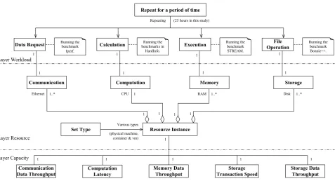
Figure 3: Experimental blueprint for evaluating three types of resources in this study.

3.10 do not support all the features for run-ning Docker containers, we choose the latest 64-bit Ubuntu 15.10 as the operating system for both the physical machine and the VM. In ad-dition, according to the discussions about base images in the Docker community [17, 18], we intentionally set an OS base image (by specifying

FROM ubuntu:15.10in the Dockerfile) for all the Docker containers in our experiments. Note that a container’s OS base image is only a file system representation, while not acting as a guest OS.

The workload-related factors:

• Duration: For each evaluation experiment, we decided to take a whole-day observation plus one-hour warming up (i.e. 25 hours).

• Workload Size: The experimental workloads are predefined by the selected benchmarks. For example, the micro-benchmark CPU Fibonacci generates workload by calculating the 42nd Fi-bonacci number (cf. Table 2). In particular, the benchmark Bonnie++ distinguishes between reading/writing byte-size and block-size data.

3.2.5 Experimental Design

It is clear that the identified factors are all with single value except for theResource Type. Therefore, a straight-forward design is to run the individual benchmarks on each of the three types of resources independently for a whole day plus one hour.

Furthermore, following the conceptual model of IaaS performance evaluation [19], we record the exper-imental design into a blueprint both to facilitate our experimental implementations and to help other eval-uators replicate/repeat our study. In particular, the

experimental elements are divided into three layers (namely Layer Workload, Layer Resource, and Layer Capacity), as shown in Figure 3. To avoid duplica-tion, we do not elaborate the detailed elements in this blueprint.

3.3 Experimental Results and Analyses

3.3.1 Communication Evaluation Result and Anal-ysis

Docker creates a virtual bridgedocker0on the host machine to enable both the host-container and the container-container communications. In particular, it is the Network Address Translation (NAT) that for-wards containers’ traffic to external networks. For the purpose of “apple-to-apple” comparison, we also con-figure VM’s network type as NAT that uses theVMnet8

virtual switch created by VMware Workstation. Using NAT, both Docker containers and VMs can establish outgoing connections by default, while they require port binding/forwarding to accept incoming connections. To reduce the possibility of configura-tional noise, we only test the outgoing communication performance, by setting the remote EC2 instance to Iperf server and using the local machine, container and VM all as Iperf clients.

(7)

There-fore, we particularly focus on the longest period of relatively stable data out of the whole-day observation, and thus the results here are for rough reference only.

Resource Type Average Standard Deviation

Physical machine 29.066 Mbits/sec 1.282 Mbits/sec Container 28.484 Mbits/sec 1.978 Mbits/sec Virtual machine 12.843 Mbits/sec 2.979 Mbits/sec

Table 3: Communication benchmarking results using Iperf.

Given the extra cost of using the NAT network to send and receive packets, there would be unavoidable performance penalties for both the container and the VM. Using Equation (1), we calculate their communica-tion performance overheads, as illustrated in Figure 4.

Physical Machine Container Virtual Machine

average 29.06630058 28.48428928 12.84306931

stdev 1.282297571 1.978326959 2.978496178

Container Virtual Machine

Variability Overhead 54.27986481 132.27808

ppp 0 0

ttt 0 0

Data Throughput Overhead 2.002357673 55.81457202

0 10 20 30 40 50 60

0 20 40 60 80 100 120 140

Container Virtual Machine

D

at

a

T

hr

ou

gh

pu

t O

ve

rh

ea

d

(%)

V

ar

iab

ili

ty

O

ve

rh

ead

(

%)

Variability Overhead Data Throughput Overhead

Figure 4: Communication data throughput and its variability overhead of a standalone Docker container vs. VM (using the benchmark Iperf).

A clear trend is that, compared to the VM, the con-tainer loses less communication performance, with only 2% data throughput overhead and around 54% variability overhead. However, it is surprising to see a more than 55% data throughput overhead for the VM. Although we have double checked the relevant configuration parameters and redone several rounds of experiments to confirm this phenomenon, we still doubt about the hypervisor-related reason behind such a big performance loss. We particularly highlight this observation to inspire further investigations.

3.3.2 Computation Evaluation Result and Analysis

Recall that HardInfo’s six micro benchmarks deliver both “higher=better” and “lower=better” CPU scores (cf. Table 2). To facilitate experimental analysis, we use the two equations below to standardize the “higher=better” and “lower=better” benchmarking

re-sults respectively.

HBi=

Benchmarkingi max Benchmarking1,2,...,n

(2)

LBi=

1 Benchmarkingi

max 1

Benchmarking1,2,...,n

! (3)

whereHBi further scores the service resource typei by standardizing the “higher=better” benchmarking result Benchmarkingi; and similarly, LBi represents the standardized “lower=better” CPU score of the ser-vice resource typei. Note that Equation (3) essen-tially offers the “lower=better” benchmarking results a “higher=better” representation through reciprocal standardization.

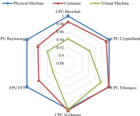
For the purpose of conciseness, here we only spec-ify the standardized experimental results, as shown in Table 4. Exceptionally, the container and VM have slightly higher CPU N-Queens scores than the physical machine. Given the predefined observational margin of error (cf. Section 3.2.3), we are not concerned with this trivial difference, while treating their performance values as equal to each other in this case.

Benchmark Physical machine Container VM

CPU Blowfish 1 0.986 0.942

CPU CryptoHash 1 0.992 0.943

CPU Fibonacci 1 0.999 0.976

CPU N-Queens 0.996 1 0.997

FPU FFT 1 0.966 0.924

FPU Raytracing 1 0.968 0.941

Table 4:Standardized computation benchmarking results using HardInfo.

We can further use a radar plot to help ignore the trivial number differences, and also help intuitively contrast the performance of the three resource types, as demonstrated in Figure 5. For example, the diff er-ent polygon sizes clearly indicate that the container generally computes faster than the VM, although the performance differences are on a case-by-case basis with respect to different CPU job types.

0.88 0.9 0.92 0.94 0.96 0.98 1 CPU Blowfish

CPU CryptoHash

CPU Fibonacci

CPU N-Queens FPU FFT

FPU Raytracing

Figure 5: Computation benchmarking results by using HardInfo.

(8)

does not even show worse variability than the phys-ical machine when running CPU CryptoHash, CPU N-Queens and FPU Raytracing. On the contrary, there is an almost 2500% variability overhead for the VM when calculating the 42nd Fibonacci number. In par-ticular, the virtualization technologies seem to be sensi-tive to the Fourier transform jobs (the benchmark FPU FFT), because the computation latency overhead and the variability overhead are relatively high for both the container and the VM.

0 2 4 6 8 10

0 500 1000 1500 2000 2500

L

at

en

cy

(

Sc

or

e)

O

ve

rh

ea

d

(%)

V

ar

ia

bi

lit

y

O

ve

rh

ea

d

(%)

Container (variability overhead) Virtual Machine (variability overhead) Container (latency (score) overhead) Virtual Machine (latency (score) overhead)

Figure 6: Computation latency (score) and its variabil-ity overhead of a standalone Docker container vs. VM (using the tool kit HardInfo).

3.3.3 Memory Evaluation Result and Analysis

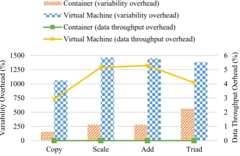
STREAM measures sustainable memory data through-put by conducting four typical vector operations, namely Copy, Scale, Add and Triad. The memory benchmarking results are listed in Table 5. We fur-ther visualize the results into Figure 7 to facilitate our observation. As the first impression, it seems that the VM has a bit poorer memory data throughput, and there is little difference between the physical machine and the Docker container in the context of running STREAM.

Operation (MB/s) Physical machine

Container VM

Copy 2902.685 2914.023 2818.291

(Std. Dev.) (4.951) (12.579) (57.633)

Scale 2916.247 2910.485 2765.737

(Std. Dev.) (3.783) (14.488) (59.193)

Add 3335.634 3332.822 3159.188

(Std. Dev.) (3.765) (14.405) (58.385)

Triad 3341.327 3340.416 3204.811

(Std. Dev.) (3.976) (26.361) (59.004)

Table 5: Memory benchmarking results using STREAM.

By calculating the performance overhead in terms of memory data throughput and its variability, we are able to see the significant difference among these three

types of resources, as illustrated in Figure 8. Take the operation Triad as an example, although the con-tainer performs as well as the physical machine on average, the variability overhead of the container is more than 500%; similarly, although the VM’s Triad data throughput overhead is around 4% only, its vari-ability overhead is almost 1400%. In other words, the memory performance loss incurred by both virtualiza-tion techniques is mainly embodied with the increase in the performance variability.

0 500 1000 1500 2000 2500 3000 3500

Copy Scale Add Triad

M

emo

ry

D

at

a

T

hr

ou

gh

pu

t (

M

B

/s)

Memory Operation by STREAM

Figure 7: Memory benchmarking results by using STREAM. Error bars indicate the standard deviations of the corresponding memory data throughput.

0 1 2 3 4 5 6

0 250 500 750 1000 1250 1500

Copy Scale Add Triad

D

at

a

T

hr

ou

gh

pu

t O

er

he

ad

(

%)

V

ar

ia

bi

lit

y

O

ve

rh

ea

d

(%)

Container (variability overhead) Virtual Machine (variability overhead) Container (data throughput overhead) Virtual Machine (data throughput overhead)

Figure 8: Memory data throughput and its variabil-ity overhead of a standalone Docker container vs. VM (using the benchmark STREAM).

In addition, it is also worth notable that the con-tainer’s average Copy data throughput is even slightly higher than the physical machine (i.e. 2914.023MB/s vs. 2902.685MB/s) in our experiments. Recall that we have considered a 1% margin of error. Since those two values are close to each other within this error margin, here we ignore such an irregular phenomenon as an observational error.

3.3.4 Storage Evaluation Result and Analysis

(9)

on both the physical machine and the container, by running “sudo bonnie++ -r 2048 -n 128 -d / -u root”. Correspondingly, the benchmarking trials are conducted with 4GB of random data on the disk. When Bonnie++ is running, it carries out various storage op-erations ranging from data reading/writing to file cre-ating/deleting. Here we only focus on the performance of reading/writing byte- and block-size data.

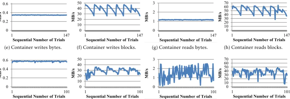
To help highlight several different observations, we plot the trajectory of the experimental results along the trial sequence during the whole day, as shown in Figure 9. The first surprising observation is that, all the three resource types have regular patterns of performance jitter in block writing, rewriting and reading. Due to the space limit, we do not report their block rewriting performance in this paper. By exploring the hardware information, we identified the hard disk drive (HDD) model to be ATA Hitachi HTS54161, and its specifi-cation describes “It stores 512 bytes per sector and uses four data heads to read the data from two plat-ters, rotating at 5,400 revolutions per minute”. As we know, the hard disk surface is divided into a set of con-centrically circular tracks. Given the same rotational speed of an HDD, the outer tracks would have higher data throughput than the inner ones. As such, those regular patterns might indicate that the HDD heads sequentially shuttle between outer and inner tracks when consecutively writing/reading block data during the experiments.

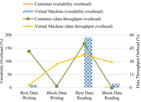
The second surprising observation is that, unlike most cases in which the VM has the worst performance, the container seems significantly poor at accessing the byte size of data, although its performance variability is clearly the smallest. We further calculate the storage performance overhead to deliver more specific com-parison between the container and the VM, and draw the results into Figure 10. Note that, in the case when the container’s/VM’s variability is smaller than the physical machine’s, we directly set the corresponding variability overhead to zero rather than allowing any performance overhead to be negative. Then, the bars in the chart indicate that the storage variability over-heads of both virtualization technologies are nearly negligible except for reading byte-size data on the VM (up to nearly 200%). The lines show that the container brings around 40% to 50% data throughput overhead when performing disk operations on a byte-by-byte basis. On the contrary, there is relatively trivial per-formance loss in VM’s byte data writing. However, the VM has roughly 30% data throughput overhead in other disk I/O scenarios, whereas the container barely incurs overhead when reading/writing large size of data.

Our third observation is that, the storage perfor-mance overhead of different virtualization technolo-gies can also be reflected through the total number of the iterative Bonnie++ trials. As pointed by the maximum x-axis scale in Figure 9, the physical ma-chine, the container and the VM can respectively fin-ish 150, 147 and 101 rounds of disk tests during 24 hours. Given this information, we estimate the

con-tainer’s and the VM’s storage performance overhead to be 2% (=|₁₄₇−₁₅₀|_/_{150) and 32}_._{67% (=}|₁₀₁−₁₅₀|_/₁₅₀₎ respectively.

0 15 30 45 60

0 50 100 150 200

Byte Data Writing

Block Data Writing

Byte Data Reading

Block Data Reading

D

at

a

T

hr

ou

gh

pu

t O

er

he

ad

(

%)

V

ar

ia

bi

lit

y

O

ve

rh

ea

d

(%)

Container (variability overhead) Virtual Machine (variability overhead) Container (data throughput overhead) Virtual Machine (data throughput overhead)

Figure 10:Storage data throughput and its variability overhead of a standalone Docker container vs. VM (using the benchmark Bonnie++).

3.4 Performance Evaluation Conclusion

Following the performance evaluation methodology DoKnowMe, we draw conclusions mainly by answer-ing the predefined requirement questions. Driven by RQ1 and RQ2, our evaluation result largely confirms the aforementioned qualitative discussions: The con-tainer’s average performance is generally better than the VM’s and is even comparable to that of the physical machine with regarding to many features. Specifically, the container has less than 4% performance overhead in terms of communication data throughput, compu-tation latency, memory data throughput and storage data throughput. Nevertheless, the container-based virtualization could hit a bottleneck of storage transac-tion speed, with the overhead up to 50%. Note that, as mentioned previously, we interpret the byte-size data throughput into storage transaction speed, because each byte essentially calls a disk transaction here. In contrast, although the VM delivers the worst perfor-mance in most cases, it could perform as well as the physical machine when solving the N-Queens prob-lem or writing small-size data to the disk. By further comparing the storage filesystems of those two types of virtualization technologies, we believe that it is the copy-on-write mechanism that makes containers poor at storage transaction speed.

(10)

0 0.2 0.4 0.6

1 150

M

B

/s

Sequential Number of Trials

(a) Physical machine writes bytes.

0 10 20 30 40 50

1 150

M

B

/s

(b) Physical machine writes blocks.

0 1 2 3

1 150

M

B

/s

(c) Physical machine reads bytes.

0 10 20 30 40 50 60 70

1 150

M

B

/s

(d) Physical machine reads blocks.

0 0.2 0.4 0.6

1 147

M

B

/s

(e) Container writes bytes.

0 10 20 30 40 50

1 147

M

B

/s

(f) Container writes blocks.

0 1 2 3

1 147

M

B

/s

(g) Container reads bytes.

0 10 20 30 40 50 60 70

1 147

M

B

/s

(h) Container reads blocks.

0 0.2 0.4 0.6

1 101

M

B

/s

(i) Virtual machine writes bytes.

0 10 20 30 40 50

1 101

M

B

/s

Sequential Number of Trials (j) Virtual machine writes blocks.

0 1 2 3

1 101

M

B

/s

Sequential Number of Trials (k) Virtual machine reads bytes.

0 10 20 30 40 50 60 70

1 101

M

B

/s

Sequential Number of Trials (l) Virtual machine reads blocks.

Figure 9: Storage benchmarking results by using Bonnie++ during 24 hours. The maximum x-axis scale indicates the iteration number of the Bonnie++ test (i.e. the physical machine, the container and the VM run 150, 147 and 101 tests respectively).

the physical machine’s when running CryptoHash, N-Queens, and Raytracing jobs.

4 Container-based

Application

Case Study and Performance

Op-timization

4.1 Motive from a Background Project

Adequate pricing techniques play a key role in success-ful Cloud computing [20]. In the de facto Cloud mar-ket, there are generally three typical pricing schemes, namely on-demand pricing scheme, reserved pricing scheme, and spot pricing scheme. Although the fixed pricing schemes are dominant approaches to trad-ing Cloud resources nowadays, spot prictrad-ing has been broadly agreed as a significant supplement for building a full-fledged market economy for the Cloud ecosystem [21]. Similar to the dynamic pricing in the electricity distribution industry, the spot pricing scheme here also employs a market-driven mechanism to provide spot service at a reduced and fluctuating price, in order to attract more demands and better utilize idle compute resources [22].

Unfortunately, the backend details behind chang-ing spot prices are invisible for most of the Cloud market participants. In fact, unlike the static and

straightforward pricing schemes of on-demand and reserved Cloud services, the market-driven mechanism for pricing Cloud spot service has been identified to be complicated both for providers to implement and for consumers to understand.

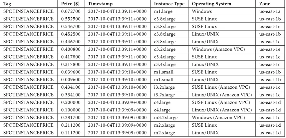
Therefore, it has become popular and valuable to take Amazon’s spot service as a practical example to investigate Cloud spot pricing, so as to encourage and facilitate more players to enter the Cloud spot market. We are currently involved in a project on Cloud spot pricing analytics by using the whole-year price his-tory of Amazon’s 1053 types of spot service instances. Since Amazon only offers the most recent 60-day price trace to the public for review, we downloaded the price traces monthly in the past year to make sure the com-pleteness of the whole-year price history.

(11)

Tag Price ($) Timestamp Instance Type Operating System Zone

SPOTINSTANCEPRICE 0.072700 2017-10-04T13:39:11+0000 m1.large Windows us-east-1a SPOTINSTANCEPRICE 0.552500 2017-10-04T13:39:11+0000 c3.8xlarge SUSE Linux us-east-1b SPOTINSTANCEPRICE 0.546700 2017-10-04T13:39:11+0000 c3.8xlarge SUSE Linux us-east-1e SPOTINSTANCEPRICE 0.452500 2017-10-04T13:39:11+0000 c3.8xlarge Linux/UNIX us-east-1b SPOTINSTANCEPRICE 0.446700 2017-10-04T13:39:11+0000 c3.8xlarge Linux/UNIX us-east-1e SPOTINSTANCEPRICE 0.400800 2017-10-04T13:39:11+0000 c3.2xlarge Windows (Amazon VPC) us-east-1e SPOTINSTANCEPRICE 0.417800 2017-10-04T13:39:11+0000 c3.4xlarge SUSE Linux us-east-1c SPOTINSTANCEPRICE 0.317800 2017-10-04T13:39:11+0000 c3.4xlarge Linux/UNIX us-east-1c SPOTINSTANCEPRICE 0.039600 2017-10-04T13:39:10+0000 m1.small SUSE Linux us-east-1b SPOTINSTANCEPRICE 0.009600 2017-10-04T13:39:10+0000 m1.small Linux/UNIX us-east-1b SPOTINSTANCEPRICE 0.434100 2017-10-04T13:39:10+0000 i3.2xlarge SUSE Linux (Amazon VPC) us-east-1c SPOTINSTANCEPRICE 0.334100 2017-10-04T13:39:10+0000 i3.2xlarge Linux/UNIX (Amazon VPC) us-east-1c SPOTINSTANCEPRICE 0.200000 2017-10-04T13:39:09+0000 c4.large SUSE Linux (Amazon VPC) us-east-1d SPOTINSTANCEPRICE 0.100000 2017-10-04T13:39:09+0000 c4.large Linux/UNIX (Amazon VPC) us-east-1d SPOTINSTANCEPRICE 0.281700 2017-10-04T13:39:09+0000 m3.2xlarge Windows (Amazon VPC) us-east-1c SPOTINSTANCEPRICE 0.211200 2017-10-04T13:39:09+0000 m2.xlarge SUSE Linux us-east-1d SPOTINSTANCEPRICE 0.111200 2017-10-04T13:39:09+0000 m2.xlarge Linux/UNIX us-east-1d

Table 6: A small piece of Amazon’s spot price trace.

4.2 WordCount-alike Solution

Given the aforementioned requirement of data clean-ing, we propose a WordCount-alike solution by analogy. WordCount is a well-known application that calculates the numbers of occurrences of different words within a document or word set. In the domain of big data analytics, WordCount is now a classic application to demonstrate the MapReduce mechanism that has be-come a standard programming model since 2004 [23]. As shown in Figure 11, the key steps in a MapReduce workflow are:



Shuffle Map

Map

Map Input

data

Output data Reduce

Reduce

Reduce Shuffle

Shuffle

Figure 11: Workflow of the MapReduce process.

(1) The initial input source data are segmented into blocks according to the predefined split function and saved as a list of key-value pairs.

(2) The mapper executes the user-defined map func-tion which generates intermediate key-value pairs.

(3) The intermediate key-value pairs generated by mapper nodes is sent to a specific reducer based on the key.

(4) Each reducer computes and reduces the data to one single key-value pair.

(5) All the reduced data are integrated into the final result of a MapReduce job.

Benefiting from MapReduce, applications like WordCount can deal with large amounts of data paral-lelly and distributedly. For the purpose of conciseness, we use a three-file scenario to demonstrate the process of MapReduce-based WordCount, as illustrated in Fig-ure 12. In brief, the input files are broken into a set of <key, value>pairs for individual words, then the<key, value>pairs are shuffled alphabetically to facilitate summing up the values (i.e. the occurrence counts) for each unique key, and the reduced results are also a set of<key, value>pairs that directly act as the output in this case.

Input:

File1: Hello World Bye World File2: Hello Docker Bye Docker File3: Hello Hadoop Bye Hadoop

Map: <Hello, 1> <World, 1> <Bye, 1> <World, 1> <Hello, 1> <Docker, 1> <Bye, 1> <Docker, 1> <Hello, 1> <Hadoop, 1> <Bye, 1> <Hadoop, 1>

Shuffle: <Bye, 1> <Bye, 1> <Bye, 1> <Docker, 1> <Docker, 1> <Hadoop, 1> <Hadoop, 1> <Hello, 1> <Hello, 1> <Hello, 1> <World, 1> <World, 1>

Output: <Bye, 3> <Docker, 2> <Hadoop, 2> <Hello, 3> <World, 2>

Reduce: <Bye, 1+1+1> <Docker, 1+1> <Hadoop, 1+1> <Hello, 1+1+1> <World, 1+1>

Figure 12: A Three-file Scenario of MapReduce-based WordCount.

Recall that the information of Amazon’s spot price trace is composed of Tag, Price, Timestamp, Instance Type and Zone (cf. Table 6). By considering the value in each information field to be a letter, we treat every

(12)

single spot price record as an English word. For ex-ample, by random analogy, the spot price record “tag price1 time1 OS1 zone1” can be viewed as a six-letter word like “Hadoop”, as highlighted in Figure 13.

Spot Price Trace File:

Tag Price1 Time1 Type1 OS1 Zone1 Tag Price2 Time2 Type2 OS3 Zone2 Tag Price3 Time3 Type1 OS1 Zone1 Tag Price4 Time4 Type3 OS2 Zone3

Word Set File (by random analogy):

H a d o o p

H b e v z q

H c f o o p

H k g w y n

Figure 13: Treating spot price records as six-letter words.

As such, we are able to follow the logic of Word-Count to fulfill the needs of cleaning our collected spot price history. In particular, instead of summing up the occurrences of the same price records, the duplicate records are simply ignored (removed). Moreover, the price records are sorted by the order of values of In-stance Type, Operating System, Zone and Timestamp sequentially during the shuffling stage, while Tag and Price are not involved in data sorting. To avoid duplica-tion, here we do not further elaborate the MapReduce-based data cleaning process.

4.3 Application Environment and

Imple-mentation

Unlike using “just-enough” environment for micro-level performance evaluation, here we employ “fair-enough” hardware resource to implement the MapReduce-based WordCount application, as listed in Table 7. In detail, the physical machine is Dell Pow-erEdge T110 II with the CPU model Intel Xeon E3-1200 series E3-1220 / 3.1 GHz. When preparing the MapRe-duce framework, we choose Apache Hadoop 2.7.0 [24] running in the operating system Ubuntu Server 16.04, and using Docker containers to construct a Hadoop cluster. In particular, Docker allows us to create an ex-clusive bridge network for the Hadoop cluster by using a specific name, e.g., sudo docker network create --driver=bridge cluster.

Environmental Item Specification

Physical Machine Dell PowerEdge T110 II Operating System Ubuntu Server 16.04 Java Environment JDK 1.8.0

MapReduce Framework Hadoop 2.7.0

Table 7: Summary of application environment.

In our initial implementation, we realized a three-node Hadoop cluster by packing Hadoop 2.7.0 into a Docker image and starting one master container and two slave ones. As illustrated in Figure 14, such a Hadoop cluster can logically be divided into a dis-tributed processing layer (i.e. MapReduce workflow) and a distributed file-system layer (i.e. Hadoop Dis-tributed File System (HDFS) in this case). When run-ning a MapReduce application, the main interactions are:



Secondary NameNode MapReduce

layer

HDFS layer

Master

DataNode TaskTracker

Slave

NameNode JobTracker

DataNode TaskTracker

Slave

Figure 14: A three-node Hadoop cluster.

(1) A MapReduce job can run in a Hadoop cluster.

(2) The JobTracker in the cluster accepts a job from the MapReduce application, and locates relevant data through the NameNode.

(3) Suitable TaskTrackers are selected and then ac-cept the tasks delivered by the JobTracker.

(4) The JobTracker communicates with the Task-Trackers and manages failures.

(5) When the collaboration among the TaskTrackers finish the job, the JobTracker updates its status and returns the result.

4.4 Performance Optimization Strategies

It is known that the performance of MapReduce ap-plications can be tuned by adjusting the various pa-rameters in the three configuration files of Hadoop. However, it is also clear that there is no one-size-fits-all approach to performance tuning. Therefore, we conducted a set of performance evaluation of our data cleaning application, in order to come up with a set of optimization strategies at least for this case.

(13)

<property>

<name>mapred.task.timeout</name> <value>60000</value>

</property>

• Turn on Out-of-Band Heartbeat.Unlike regular heartbeats, the out-of-band heartbeat is triggered when a task is complete or failed. As such, Job-Tracker will be noticed the first time when there are free resources, so as to assign them to new tasks and eventually to save time. The config-uration for turning on out-of-band heartbeat is specified as follows.

<name>mapreduce.tasktracker. outofband.heartbeat</name> <value>true</value>

</property>

• Setting Buffer.To begin with, we are concerned with a threshold percentage of buffer, and a back-ground thread will be issued to spill buffer con-tents to hard disk when the threshold is reached. Inspired by the storage micro-benchmarking re-sults (cf. Section 3.3.4), we decided to increase the threshold from 80% to 90% of buffer. As for the amount of memory to be buffer size, we double the default value (i.e. 100MB) for an intu-itive test. These two parameters can be adjusted respectively as shown below.

<name>io.sort.spill.percent</name> <value>0.9</value>

</property> <property>

• Merging Spilled Streams. As a continuation of spilling buffer contents to hard disk, the inter-mediate streams from multiple spill threads are merged into one single sorted file per partition which is to be fetched by reducers. Thus, we can control how many of spills will be merged into one file at a time. Since the smaller merge factor incurs more parallel merge activities and more disk IO for reducers, we decided to increase the merge value from 10 to 100, as shown below.

<name>io.sort.factor</name> <value>100</value>

</property>

• LZO Compression. Recall that the data we are dealing with are plain texts. The text data can generally be compressed significantly to reduce the usage of hard disk space and transmission bandwidth, and correspondingly to save the time

taken for data copying/transferring. As a loss-less algorithm with high decompression speed, Lempel-Ziv-Oberhumer (LZO) is one of the com-pression mechanisms supported by the Hadoop framework. In addition to various benefits and characteristics in common, LZO’s block structure is particularly split-friendly for parallel process-ing in MapReduce jobs [25]. Therefore, we install and enable LZO for Hadoop by specifying the configurations below.

<property>

<name>io.compression.codecs</name> <value>org.apache.hadoop.io.compress.

GzipCodec,org.apache.hadoop. io.compress.DefaultCodec, com.hadoop.compression.lzo.

LzoCodec,com.hadoop. compression.lzo.LzopCodec, org.apache.hadoop.io.compress.

BZip2Codec</value> </property>

<name>io.compression.codec. lzo.class</name> <value>com.hadoop.compression.

lzo.LzoCodec</value> </property>

<name>mapreduce.map.output. compress</name> <value>true</value>

</property> <property>

<name>mapreduce.map.output.

compress.codec</name> <value>com.hadoop.compression.

lzo.LzoCodec</value> </property>

• Doubling Slave Nodes. In distributed comput-ing, a common scenario is to employ more re-sources to deal with more workloads. Recall that map and reduce tasks of a MapReduce job are distributed to the slave nodes in a Hadoop clus-ter, and the physical machine used in this study has a Quad-Core processor. To obtain some quick clues at this current stage, we try to improve our application’s performance by doubling the slave nodes, i.e. extending the original three-node clus-ter (with two slave nodes) into a five-node one (with four slave nodes). Note that, in this opti-mization strategy, we keep the other configura-tions settings by default.

4.5 Performance Evaluation Results

(14)

these optimization strategies, we are concerned with 2GB+ and 5GB+ data respectively in the performance evaluation. Correspondingly, we draw the evaluation results in Figure 15 and 16 respectively.

0 8 16 24 32 40 48

0 20 40 60 80 100 120

Pe

rf

or

man

ce

Imp

ro

ve

me

nt

(

%

)

Ex

ec

ut

io

n

T

ime

(

s)

Execution Time Performance Improvement

Figure 15: Performance optimization for 2GB+ data cleaning.

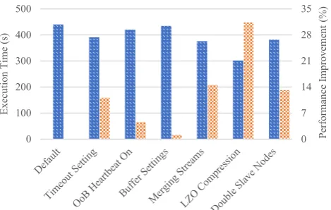
The results show three relatively different patterns of optimization effects. First, LZO compression acts as the most effective optimization strategy, and it can improve the performance nearly by 50% when dealing with 2GB+ data. Second, we can expect similar and moderate performance improvement by three individ-ual strategies, such as merging more spilled streams, reducing the timeout value, and doubling the slave nodes. Third, out-of-band heartbeat and buffer set-tings seem not to be influential optimization strategies in this case.

These different optimization patterns could be closely related to the data characteristics of our appli-cation. On one hand, since text data can be compressed significantly [26], our application mostly benefits from the optimization strategy of LZO compression. On the other hand, since the current price traces used in this study are still far from “big data”, the buffer setting could not take clear effects until the data size reaches TB levels.

0 7 14 21 28 35

0 100 200 300 400 500

Pe

rf

or

man

ce

Imp

ro

ve

me

nt

(

%)

Ex

ec

ut

io

n

T

ime

(

s)

Execution Time Performance Improvement

Figure 16: Performance optimization for 5GB+ data cleaning.

5 Related Work

Although the performance advantage of containers were investigated in several pioneer studies [3, 27, 10], the container-based virtualization solution did not gain significant popularity until the recent underlying im-provements in the Linux kernel, and especially until the emergence of Docker [28, 29]. Starting from an open-source project in early 2013 [7], Docker quickly becomes the most popular container solution [2] by significantly facilitating the management of containers. Technically, through offering the unified tool set and API, Docker relieves the complexity of utilizing the relevant kernel-level techniques including the LXC, the cgroup and a copy-on-write filesystem. To exam-ine the performance of Docker contaexam-iners, a molecular modeling simulation software [30] and a postgreSQL database-based Joomla application [31] have been used to benchmark the Docker environment against the VM environment.

Considering the uncertainty of use cases (e.g., dif-ferent workload densities and QoS requirements), at this current stage, a baseline-level investigation would be more useful and helpful for understanding the fun-damental difference in performance overhead between those two virtualization solutions. A preliminary study has particularly focused on the CPU consumption by using the 100000! calculation within a Docker con-tainer and a KVM VM respectively [32]. Nevertheless, the concerns about other features/resources like mem-ory and disk are missing. Similarly, the performance analysis between VM and container in study [33] is not feature-specific enough (even including security that is out of the scope of performance). On the con-trary, by treating Docker containers as a particular type of Cloud service, our study considers the four physi-cal properties of a Cloud service [15] and essentially gives a fundamental investigation into the Docker con-tainer’s performance overhead on a feature-by-feature basis.

The closest work to ours is the IBM research report on the performance comparison of VM and Linux con-tainers [34]. In fact, it is this incomplete report (e.g., the container’s network evaluation is partially miss-ing) that inspires our study. Surprisingly, our work denies the IBM report’s finding “containers and VMs impose almost no overhead on CPU and memory us-age” that was also claimed in [35], and we also doubt about “Docker equals or exceeds KVM performance in every case”. In particular, we are more concerned with the overhead in performance variability.

(15)

container-based MapReduce cluster in a specific appli-cation scenario.

Note that, although there are also performance studies on deploying containers inside VMs (e.g., [36, 37]), such a redundant structure might not be suitable for an “apple-to-apple” comparison between Docker containers and VMs, and thus we do not in-clude this virtualization scenario in our study.

6 Conclusions and Future Work

It has been identified that virtualization is one of the foundational elements of Cloud computing and helps realize the value of Cloud computing [38]. On the other hand, the technologies for virtualizing Cloud infrastructures are not resource-free, and their perfor-mance overheads would incur negative impacts on the QoS of the Cloud. Since hypervisors that currently dominate the Cloud virtualization market are a rela-tively heavyweight solution, there comes a rising trend of interest in its lightweight alternative [7], namely the container-based virtualization. Their mechanism difference is that, the former manages the host hard-ware resources, while the latter enables sharing the host OS. Although straightforward comparisons can be done from the existing qualitative discussions, we conducted a fundamental evaluation study to quan-titatively understand the performance overheads of these two different virtualization solutions. In particu-lar, we employed a standalone Docker container and a VMWare Workstation VM to represent the container-based and the hypervisor-container-based virtualization tech-nologies respectively.

Recall that there are generally two stages of per-formance engineering in ECS, for revealing the pri-mary performance of specific (system) features and investigating the overall performance of real-world applications respectively. In addition to the fundamen-tal performance of a single container, we also studied performance optimization of a container-based MapRe-duce application in terms of cleaning Amazon’s spot price history. At this current stage, we only focused on one factor at a time to evaluate the optimization strategies ranging from setting task timeout to dou-bling slave nodes.

Overall, our work reveals that the performance overheads of these two virtualization technologies could vary not only on a feature-by-feature ba-sis but also on a job-to-job baba-sis. Although the container-based solution is undoubtedly lightweight, the hypervisor-based technology does not come with higher performance overhead in every case. At the application level, the container technology is clearly more resource-friendly, as we failed in building VM-based MapReduce clusters on the same physical ma-chine. When it comes to container-based MapReduce applications, it seems that the effects of performance optimization strategies are closely related to the data characteristics. For dealing with text data in our case study, LZO compression can bring the most significant

performance improvement.

Due to the time and resource limit, our current in-vestigation into the performance of container-based MapReduce applications is still an early study. Thus, our future work will be unfolded along two directions. Firstly, we will adopt sophisticated experimental de-sign techniques (e.g., the full-factorial dede-sign) [39] to finalize the same case study on tuning the MapReduce performance of cleaning Amazon’s price history. Sec-ondly, we will gradually apply Docker containers to different real-world applications for dealing with dif-ferent types of data. By employing “more-than-enough” computing resource, the application-oriented practices will also be replicated in the hypervisor-based virtual environment for further comparison case studies.

Acknowledgment This work is supported by the Swedish Research Council (VR) under contract number C0590801 for the project Cloud Control, and through the LCCC Linnaeus and ELLIIT Excellence Centers. This work is also supported by the National Natural Science Foundation of China (Grant No.61572251).

References

[1] Z. Li, M. Kihl, Q. Lu, and J. A. Andersson, “Performance over-head comparison between hypervisor and container based vir-tualization,” inProceedings of the 31st IEEE International Confer-ence on Advanced Information Networking and Application (AINA 2017). Taipei, Taiwan: IEEE Computer Society, 27-29 March 2017, pp. 955–962, https://doi.org/10.1109/AINA.2017.79. [2] C. Pahl, “Containerization and the PaaS Cloud,”IEEE Cloud

Computing, vol. 2, no. 3, pp. 24–31, May/June 2014, https: //doi.org/10.1109/MCC.2015.51.

[3] J. P. Walters, V. Chaudhary, M. Cha, S. G. Jr., and S. Gallo, “A comparison of virtualization technologies for HPC,” in Pro-ceedings of the 22nd International Conference on Advanced Infor-mation Networking and Applications (AINA 2008). Okinawa, Japan: IEEE Computer Society, 25-28 March 2008, pp. 861–868, https://doi.org/10.1109/AINA.2008.45.

[4] P. J. Denning, “Performance evaluation: Experimental com-puter science at its best,” ACM SIGMETRICS Performance Evaluation Review, vol. 10, no. 3, pp. 106–109, Fall 1981, https://doi.org/10.1145/1010629.805480.

[5] D. G. Feitelson, “Experimental computer science,” Communi-cations of the ACM, vol. 50, no. 11, pp. 24–26, November 2007, https://doi.org/10.1145/1297797.1297817.

[6] Z. Li, L. O’Brien, and M. Kihl, “DoKnowMe: Towards a do-main knowledge-driven methodology for performance eval-uation,”ACM SIGMETRICS Performance Evaluation Review, vol. 43, no. 4, pp. 23–32, 2016, https://doi.org/10.1145/ 2897356.2897360.

[7] D. Merkel, “Docker: Lightweight Linux containers for consis-tent development and deployment,”Linux Journal, vol. 239, pp. 76–91, March 2014.

[8] X. Xu, H. Yu, and X. Pei, “A novel resource scheduling approach in container based clouds,” inProceedings of the 17th IEEE In-ternational Conference on Computational Science and Engineer-ing (CSE 2014). Chengdu, China: IEEE Computer Society, 19-21 December 2014, pp. 257–264, https://doi.org/10.1109/ CSE.2014.77.