DISCRETE WAVES
LAURA JAMES
ADVISOR: HANS CHRISTIANSON
Abstract. We study the discrepancies between the continuous versus discretized wave equations. Motivated by the theoretical study of so-called “spurious” high-frequency wave packets initiated in [1], we use the finite difference algorithm to approximate solutions to a one-dimensional wave equation onS1at low and high frequencies. We numerically compare these approximate solutions
to the explicit continuous solutions using the discrete analog of the usual wave energy. For low frequencies there is good agreement, while for high frequencies there is very bad agreement. We explain this high frequency phenomenon heuristically by observing that, for initial data resulting in propagation in one direction only, the approximate solution nevertheless has non-trivial wave packets propagating in both directions.
1. Introduction
In this paper, we are concerned with a phenomenon which occurs with the numerical study of high frequency waves. In order to show this phenomenon, we study the wave equation on [0,1] with periodic boundary conditions using two different methods.
utt−uxx= 0
u(t,0) =u(t,1)
ux(t,0) =ux(t,1)
u(0, x) =f(x)
ut(0, x) =g(x) (1.1)
In the first method, we discretize on a uniform mesh with N subdivisions of lengthh= N1. We use the usual finite difference matrixAand solve the resulting ODE’s to get an approximation of the solution to (1.1). In the second method, we solve the wave equation in the continuum and then sample the solution on our mesh. The energy
(1.2) E(t) =
Z 1
0
(|ut|2+|ux|2)dx
is known to be conserved for (1.1) (see Appendix A). If~u is a discretized approximate solution, then the discrete analog of (1.2) is
(1.3) E(~u) =~ut·~ut+ (A~u)·~u,
which we use to calculate the discrete energy for the approximate solution using each method. Not surprisingly, the energy is (almost) conserved using each method. Additionally, the energy in the first method is very close to the energy in the second method. However, something interesting
occurs when we examine the energy of the difference of the two approximate solutions. For low frequencies, the energy of the difference is relatively small. On the other hand, for high frequencies the energy of the difference is much larger. This is numerical confirmation of the defects seen in high frequency discrete waves. This phenomenon was first observed numerically but the high frequencies were “truncated” (see, for example, the survey article [4] and the references therein). [1] explains theoretically what happens with these high frequencies.
1.1. Acknowledgements. We programmed the algorithms used in this project from scratch, which was very time consuming. Additionally, computer time was limited. Therefore, it took too much time to be able to study geometric control for the damped wave equation, which was our original motivation [1]. I would like to extend a special thanks and appreciation to my advisor Hans Christianson for his guidance on this project. Also, thank you to Jason Metcalfe, Jeremy Marzuola, and Hans Christianson for serving on the committee.
2. Descriptions of the Two Methods
2.1. First Method. It should be noted that we do not use any built-in functions (other than sqrt, exp, dot, andzeros) or algorithms in MATLAB, as they may have added features which we do not want in our method. In the first method, we discretize first. Our discretization occurs on a uniform mesh with N subdivisions of lengthh= N1.
0 h 2h. . . (N−1)h 1
We use the second order finite difference matrix
A= 1
h2
2 −1 0 . . . −1
−1 2 −1 0 . . . 0 0 −1 2 −1 0 . . . 0
..
. . ..
−1 0 . . . 0 −1 2
to approximate −∂x∂22 (see Appendix B).
Our discrete solution can be written as the discrete Fourier series
(2.1) U~ =X
j Uj~ej
where
~ej= √
h
e2πijh∗0 e2πijh∗1
.. .
e2πijh∗(N−1)
is the basis of orthonormal eigenvectors of A with eigenvalues µ
2
j h2
A~ej= 2−2 cos(2πjh)
h2 ~ej (see Appendix C)
= µ
2 j h2~ej
(2.2)
andUj is given by
Uj =hU , ~~ eji.
Our wave equation then becomes the discretized wave equation
(2.3) U~ 00+A ~U =X
j
Uj00~ej+
X
j µ2j
h2Uj~ej = 0
with initial conditions
~
U(0) =F~
~
U0(0) =G.~
Notice that the boundary conditions are contained inA. By matching the coefficients in (2.3) we see that
Uj00=−µ 2 j h2Uj,
and solving this ODE gives us a formula forUj.
(2.4) Uj=Cj+e
iµj
h t+Cj−e −iµj
h t
Now let’s also sample our initial conditions and write them as a discrete Fourier series. We will compare to the continuum dataf, g later.
(2.5) F~ =X
j Fj~ej
(2.6) G~ =X
j Gj~ej
Using (2.1), (2.4), (2.5), and (2.6), we obtain formulas forFj andGj.
~
U(0) =X
j
(Cj++Cj−)~ej=F~
~
U0(0) =X
j
iµj
h Cj+− iµj
h Cj−
~ ej =G~
Therefore,
(2.7) Fj =Cj++Cj−
(2.8) Gj =iµj
h Cj+− iµj
2.2. Second Method. In the second method, we solve the wave equation in the continuum and then discretize. We can explicitly write out the solution as
(2.9) u=X
n
Dn+e2πint+Dn−e−2πint
e2πinx
with initial conditions
(2.10) u(0, x) =f(x) =X
n
fne2πinx
(2.11) ut(0, x) =g(x) =X
n
gne2πinx.
Using (2.9), (2.10), and (2.11), we obtain formulas forfn andgn.
u(0) =X
n
Dn++Dn−
e2πinx=f(x)
ut(0) =
X
n
2πinDn+−2πinDn−
e2πinx=g(x)
Therefore,
(2.12) fn=Dn++Dn−
(2.13) gn= 2πinDn+−2πinDn−
2.3. Choice of Frequencies. Now that we have both of our methods set up, we must determine what frequencies to use in order to illustrate the phenomenon. For our numerical experiments we need a narrow band of low frequencies as well as a narrow band of high frequencies, and both bands should not be too computationally expensive to use. The low frequency band should be near zero where the eigenvalues of both methods are very close. Therefore, we want a range where 2πn is very close to µj
h. We can study the Taylor expansion of µj
h in order to determine what range to
pick.
µj h =
(2−2 cos (2πjh))1/2
h
=
√
2
h
h
1−(1−(2πjh) 2
2 +O((jh)
4))i1/2
=
√
2
h
(2πjh)2 2
1/2h
1 +O((jh)2)i
1/2
= 2πj(1 +O(j2h2)) = 2πj+O(j3h2)
Our algorithm error isO(h), which is the mesh size. This is one order of magnitude worse than the
O(h2) error in the more modern finite element method (see, for example, [3]). Therefore, a relative
error in our Taylor series ofO(h1+) for >0 is sufficient as long as N is big enough. We choose O(h2) because of our computer resources. Since O(j3h2) = O(h2) if j is bounded independent
For our high frequency range we choose N−20 ≤j ≤N −1. By periodicity, these µj are close toµj for 1≤j≤20 and will therefore be small. However, since 2πngrows linearly in n, 2πnwill be much larger than µj
h in this high frequency range. In other words, we expect good agreement
of the eigenvalues in each method at low frequencies, but bad agreement at high frequencies. Our way of measuring this is to use the energy.
3. Numerical Experiments
3.1. Low Frequency Experiments. We now compute the low frequency approximate solution using each method, as well as compute the energy of the difference of the solutions. We write a program in MATLAB that computes all of the following equations. For simplicity we take specific frequency-localized initial dataf, g. To single out the low frequencies we take
Dn−= 0∀n
Dn+=
(
1, 1≤n≤20 0, otherwise
so that the wave only propagates in one direction. This determinesfn andgn.
(3.1) fn=
(
1, 1≤n≤20 0, otherwise
(3.2) gn=
(
2πin, 1≤n≤20 0, otherwise
Our solution in the continuum is therefore
(3.3) u=
20
X
n=1
e2πinte2πinx=
20
X
n=1
e2πin(x+t)
and
(3.4) ut=
20
X
n=1
(2πin)e2πinte2πinx.
We now discretize u by sampling it on our mesh. We call itw~:
~ w= √1
h 20
X
n=1
e2πint~en.
We also sampleut and call itwt. Notice thatwt~ is the same no matter if we sampleutor take∂t
ofw~.
~ wt=
1
√ h
20
X
n=1
(2πin)e2πint~en.
We renormalizew~ andwt~ by multiplying both equations by √h.
(3.5) w~ =
20
X
n=1
(3.6) wt~ =
20
X
n=1
(2πin)e2πint~en
On the other hand, we samplef andgand call themF~1andG~1.
~ F1=
20 X n=1 ~ en ~ G1=
20
X
n=1
(2πin)~en
This determinesCn+ andCn− in the first method and we can therefore explicitly write outU~ and ~
Ut.
(3.7) Cn+=
1 2
1 + h
µn ·2πn
(3.8) Cn−=
1 2
1− h µn
·2πn
(3.9) U~ =
20
X
n=1
h
Cn+e iµn
h t+Cn−e −iµn
h t
i
~en
(3.10) U~t=
20
X
n=1
hiµn
h Cn+e iµn
h t−iµn h Cn−e
−iµn h t
i
~ en
Notice that for 1≤n≤20,Cn−is small and therefore the wave mostly propagates in one direction.
This is similar to the continuous case in (3.3), which is a function ofx+tand therefore propagates to the left only. We use Hamiltonian flow to explain the propagation rule x−x0=±tin section
4.
Next we compute the energy of the approximate solutions at timest= 0, πh,2πh, . . . ,(N−1)πh. The times must be irrational so that the time evolution is not periodic.
(3.11) E(U~) =Ut~ ·Ut~ + (A ~U)·U~
(3.12) E(w~) =w~t·w~t+ (A ~w)·w~
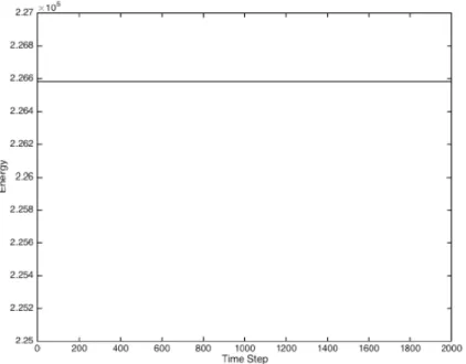
We run our experiments for several values of N, and we find that the energy is (almost) conserved within each method as well as between the two methods∗. For example, Figure 1 shows the energy at each time using the first method and Figure 2 shows the energy at each time using the second method forN = 2000.
Figure 1. Energy of U~ forN = 2000 using the low frequency band 1≤n≤20. The
same experiment was run for N = 100, 200, 300, . . ., 2000, 2500, 3000,. . . , 5000 and the picture is similar.
Figure 2. Energy of w~ forN = 2000 using the low frequency band 1 ≤n≤20. The
We also examine the energy of the difference of the two approximate solutions.
(3.13) E(U~ −w~) = (U~t−w~t)·(U~t−w~t) + (A(U~ −w~))·(U~ −w~)
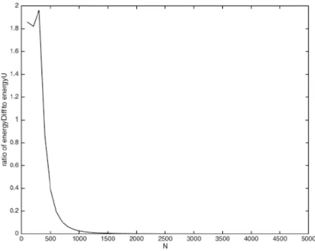
We find that as N increases, the energy of the difference becomes small relative toE(U~). This fact
is obvious when we graph the ratios E(U~−w~)((N−1)πh)
E(U~)((N−1)πh) for different values of N.
Figure 3. Ratio of the energy of U~ −w~ to the energy of U~ at the last time step for
increasing N using the low frequency band 1≤n≤20. Ratios were computed forN = 100, 200, 300,. . ., 2000, 2500, 3000,. . ., 5000.
3.2. High Frequency Experiments. We now run the exact same experiments with the high frequency band near N†. This time,Cn
−in (3.8) is large and therefore the wave propagates in both
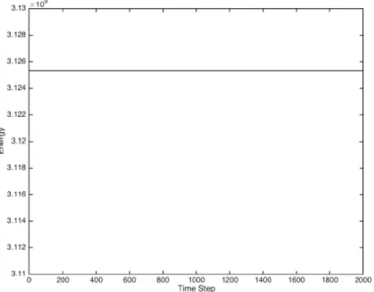
directions. We again compute the energy of the approximate solution from each method as well as the energy of the difference. Again, we find that the energy is (almost) conserved within each method as well as between the two methods. This is shown in Figure 4 and Figure 5.
Figure 4. Energy ofU~ forN= 2000 using the high frequency bandN−20≤n≤N−1. The same experiment was run forN = 100, 200, 300,. . ., 2000, 2500, 3000,. . . , 5000 and the picture is similar.
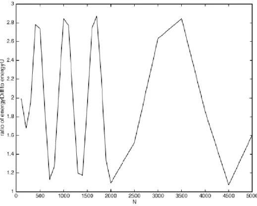
However, we observe that as N becomes large, the energy of the difference is on the same order
of magnitude asE(U~). We graph the ratios E(U~−w~)((N−1)πh)
E(U~)((N−1)πh) , which are all order 10
0. The ratios
clearly do not decay to zero as N increases.
Figure 6. Ratio of the energy of U~ −w~ to the energy of U~ at the last time step for
increasing N using the high frequency bandN−20≤n≤N−1. Ratios were computed forN= 100, 200, 300,. . ., 2000, 2500, 3000,. . ., 5000.
4. Hamiltonian Flow
We can explain this phenomenon of defects seen in high frequency discrete waves by studying the Hamiltonian Flow of the continuous case versus the discrete case. It is well known that waves propagate along the Hamiltonian flow of the principal symbol of the wave equation,τ2−ξ2[2] (See
Appendix D). For low frequencies (near zero), the discrete wave propagates close to the continuous wave. However, for high frequencies (near N), propagation in the discrete case is much different than in the continuous case. The Hamiltonian in the continuum is given by
whereξ= 2πnandn6= 0. Our Hamiltonian ODE’s are ˙
ξ=−Hx= 0 ˙
τ =−Ht= 0
˙
t=Hτ = 2τ
˙
x=Hξ =−2ξ
(4.2)
and solving gives us
ξ=ξ0
τ =τ0
t=t0+ 2τ0s
x=x0−2ξ0s.
(4.3)
We taket0= 0. We also avoidξ0= 0 andτ0= 0 so that we can solve fors.
s=x0−x 2ξ0
= t
2τ0
Waves live whereHc= 0 and thereforeτ =±ξ. This gives us x0−x
2ξ0
= ±t 2ξ0
or
(4.4) x−x0=±t.
Notice that the wave always has constant speed 1 no matter the frequency.
In the discrete case, our eigenvalues in (2.2) can be written as h42sin
2
(πhj) using trig identities. The Hamiltonian is therefore given by
Hd=τ2− 4 h2sin
2(πhj)
=τ2− 4 h2sin
2hξ
2
.
(4.5)
The Hamiltonian ODE’s in this case are ˙
ξ=−Hx= 0 ˙
τ=−Ht= 0
˙
t=Hτ = 2τ
˙
x=Hξ = −4
h sin
hξ 2
coshξ 2
(4.6)
and solving gives us
ξ=ξ0
τ =τ0
t=t0+ 2τ0s
x=x0−s
4
hsin
hξ 2
coshξ
2
.
For low frequencies near zero,
˙
x=−4
h sin
hξ 2
coshξ 2
=−4
h sin(πhj) cos(πhj) −4
h · hξ
2 ·1 =−2ξ,
which is equal to ˙xin (4.2) and therefore the discrete case propagates close to the continuous case for low frequencies.
For high frequencies near N,
˙
x=−4
h sin(πhj) cos(πhj) 0.
Appendix A. Energy Conservation for Wave Equation
We show energy conservation for the wave equation
utt−uxx= 0
u(t,0) =u(t,1)
ux(t,0) =ux(t,1)
u(0, x) =f(x)
ut(0, x) =g(x).
We define the energy as
E(t) = Z 1
0
(|ux|2+|ut|2)dx.
To show energy conservation, we need to showE0(t) = 0. We compute
E0(t) = Z 1
0
(uxuxt+uxtux+ututt+uttut)dx
= 2Re
Z 1
0
(uxuxt+uttut)dx.
We integrate by parts inx.
E0(t) = 2Re
Z 1
0
(−uxxut+uttut)dx+uxut
1
0
The periodic boundary conditions
u(t,0) =u(t,1)
ux(t,0) =ux(t,1)
are independent of t. Hence,
ut(t,0) =ut(t,1).
So
ux(t,0)ut(t,0) =ux(t,1)ut(t,1)
and we are left with
E0(t) = 2Re
Z 1
0
(utt−uxx)utdx
= 0
Appendix B. Derivation of Second Difference Matrix A
We sample a functionuon a mesh of size h to get a vector with h1 components.
~ u= u0 u1 .. . uN−1
, uj =u(jh)
We approximate the derivatives using difference quotients. The first derivative is approximated by
u0(jh)'u((j+ 1)h)−u(jh)
h .
The second derivative is then approximated by
u00(jh)' u
0((j+ 1)h)−u0(jh) h
=
u((j+1)h)−u(jh))
h
−u(jh)−uh((j−1)h) h
= u((j+ 1)h)−2u(jh) +u((j−1)h)
h2
= uj+1−2uj+uj−1
h2 .
Since we are indexing ~ustarting at zero, this formula works for 1 ≤ j ≤N −2. For j = 0 and
j=N−1 we need to use the periodic boundary conditions. That is, sinceu(t,0) =u(t,1), when we discretize we identify u0 with uN and u−1 with uN−1. Thus for j = 0, u1 −2u0+u−1 = u1−2u0+uN−1and similarly forj =N−1. Therefore,
−∂2 ∂x2u≈
1 h2
2 −1 0 . . . −1
−1 2 −1 0 . . . 0 0 −1 2 −1 0 . . . 0 ..
. . ..
−1 0 . . . 0 −1 2 ~ u.
Appendix C. Eigenvalues of MatrixA
We define the vectorsej~ to be
~ ej =√h
e2πijh∗0 e2πijh∗1
.. .
e2πijh∗(N−1)
.
The√hfactor makes the vectors orthonormal, that is
~
We apply matrixAto ej~:
A ~ej= 1
h2
2 −1 0 . . . −1
−1 2 −1 0 . . . 0 0 −1 2 −1 0 . . . 0 ..
. . ..
−1 0 . . . 0 −1 2 √ h
e2πijh∗0 e2πijh∗1
.. .
e2πijh∗(N−1)
The kth entry is
(A ~ej)k = √
h
−(e2πijh)k−1+ 2(e2πijh)k−(e2πijh)k+1 h2
=√h
−e2πijhke−2πijh+ 2e2πijhk−e2πijhke2πijh h2
=√h
(2−e−2πijh−e2πijh)e2πijhk h2
Notice
e−2πijh+e2πijh= (cos(−2πjh)) +isin(−2πjh)) + (cos(2πjh) +isin(2πjh)) = 2 cos(2πjh).
So
(A ~ej)k = √
h
2
−2 cos(2πjh))
h2 e 2πijhk
and therefore
A ~ej= 2−2 cos(2πjh)
h2 ej.~
In other words, the collection{ej}~ are eigenvectors with eigenvaluesµ2j h2 =
2−2 cos(2πjh)
h2 . Hence
they constitute an orthonormal basis ofRN of eigenvectors of the matrixA.
Appendix D. Derivation of Symbols
Fourier series replaces differentiation with multiplication. Take, for example, the Fourier series of a functionG(x).
G(x) =X
n
Gne2πinx
Gn=hG(x), e2πinxi
If we differentiateG(x) twice, we get:
∂x2G(x) =X
n
Gn(2πin)2e2πinx
=X
n
−(2πn)2Gne2πinx
For the wave equation, we take:
(∂t2−∂ 2
x)u(t, x) = (∂ 2 t−∂
2 x)
X
n
un(t)e2πinx= 0
=∂t2X n
un(t)e2πinx+X
n
(2πn)2un(t)e2πinx
=X
n
[u00n(t) + (2πn)2un(t)]e2πinx
Therefore for each n,
∂t2un(t) + (2πn)2un= 0.
We take the Fourier transform in time:
F(∂t2un(t) + (2πn)2un) =√1
2π
Z ∞
−∞
e−iτ t(∂t2un(t) + (2πn)2un)dt= 0
To solve this integral, we formally integrate by parts twice:
= √1
2π
Z ∞
−∞
−∂te−iτ t∂tun+e−iτ t(2πn)2undt
= √1
2π
Z ∞
−∞
∂t2e−iτ tun+e−iτ t(2πn)2undt
= √1
2π
Z ∞
−∞
[−τ2un+ (2πn)2un]e−iτ tdt
This is the definition of the Fourier transform of−τ2un+ (2πn)2un. Hence, −τ2unˆ + (2πn)2unˆ = (−τ2+ξ2)ˆun= 0
Therefore the symbol for the wave equation in the continuum is
−τ2+ξ2
or
τ2−ξ2.
For the discrete case, we have
(∂t2+A)U~ = 0 or
X
n
(∂t2+A)Un(t)e~n=
X
n
Un00e~n+
X
n µ2
n
h2Une~n= 0.
Now the eigenvalues are µ2n h2 =
4 h2sin
2(πhn) instead of (2πn)2. Hence, the symbol for the wave
equation in the discrete case is
τ2− 4 h2sin
2
(πhn) or
τ2− 4 h2sin
2(hξ
References
[1] H. Christianson and F. Mac`ıa. Semiclassical measures and observability for discrete waves.in preparation, 2016. [2] L. H¨ormander. Fourier integral operators. I.Acta Math., 127(1-2):79–183, 1971.
[3] G. Strang.Computational science and engineering. Wellesley-Cambridge Press, Wellesley, MA, 2007.