Bulletin of Mathematical Analysis and Applications ISSN: 1821-1291, URL: http://www.bmathaa.org Volume 8 Issue 3(2016), Pages 78-110.
THE Du-CLASSICAL ORTHOGONAL POLYNOMIALS
(COMMUNICATED BY FRANCISCO MARCELLAN)
ATEF ALAYA
Abstract. TheDu-classical orthogonal polynomial sequences are defined through
theDu-Hahn’s property: sequences that are orthogonal together with their
Du-first derivative, where Du(p) =p0+uθ0p,for allp ∈C[X]. We charac-terize them by means of a functional equation, aDu-second order linear
dif-ferential equation, the first and the second structure relations. ADu-classical
orthogonal sequence is especially a D-Laguerre-Hahn sequence of class less than or equal to two. A complete classification of theDu-classical sequences
is obtained. The functional equation coefficients, the structure relations coef-ficients, the three-term recurrence relation coefficients and the class are when-ever given.
1. introduction
Lot of works dealing with orthogonal polynomials mention the very classical ones: continuous (Hermite, Laguerre, Bessel and Jacobi), discrete (Charlier, Meixner, Krawtchouk and Hahn) or their analogues with respect to lowering difference or differential operators (Hahn operator, Delta operator, Dunkl operator, etc..) [14], [18], [19], [32], [36], [47], [49], [51], [55], and [11], [13], [15], [35], [56].
Rodrigues formula, Hahn property, Bochner condition, first and second structure relations, and Pearson equation are important common tools to characterize and construct these polynomial sequences [1], [4], [6], [7], [8], [14], [18], [22], [26], [30], [32], [36], [37], [49], [50], [51], [57], [63], [20]. In fact, using these tools, different unified presentations of classical orthogonal polynomials are done in the literature either for continuous case, discrete case or their analogues: through an algebraic approach [47], [49], a functional approach [26], [39], a distributional approach [27], [53], a hypergeometrical approach [9], [33], a difference calculus approach [19], a matrix approach [63], etc...[44]
Besides, different natural procedures are used to build new orthogonal polyno-mial sequences (see [2], [5], [10], [13], [18], [21], [23], [24], [25], [38], [40], [46], [48]
2010Mathematics Subject Classification. 33C45, 42C05.
Key words and phrases. linear functionals; Orthogonal polynomials; Laguerre-Hahn
polynomials. c
2016 Universiteti i Prishtin¨es, Prishtin¨e, Kosov¨e.
Submitted February 19, 2016. Published September 2, 2016.
A. Alaya was supported by Institute of Scientific Research and Revival of Islamic Heritage at Umm Al-Qura University (Project ID 43305032), Saudi Arabia.
u
and [54]). They start by using some classical polynomials and yield a lot of poly-nomial sequences but generally with no apparent link between them. In front of the accumulation of the obtained results of such procedures, the need of structure and classification of orthogonal polynomial sequences was natural. Among others, the papers [9], [12], [23], [25], [28], [31], [44], [34], [35], [41], [43], [45] and [46] pro-vide sketches in this direction highlighting the so-called semiclassical polynomial sequences, and where classical orthogonal polynomials are seen as semiclassical ones of class zero. In the same context, in [33] the authors emphasize the hyper-geometric character rather than the sequences therein. An algebraic approach is also presented in [47] for the so-called Laguerre-Hahn polynomials generalizing the semiclassical case. Some early tries worthy of being evoked too in the same object are [59], [60] and [61].
All these works usually give orthogonal polynomials generalizing (by their prop-erties and their characterizations) the classical orthogonal polynomials, but gener-ally it is difficult to explicitly construct them except under further assumptions as the symmetry [2], [3], [16], [17], [29], [52], [57], [58] and [62].
The aim of this work is to pick up orthogonal polynomial sequences under a
low-ering operator denoted byDu, generalizing the standard derivative D= dxd. This
operator was first introduced to see all Laguerre-Hahn polynomials of class zero,
build in [16], as the unique solutions ofDu Hahn’s property. In [42], the authors
define the Du-semiclassical polynomials and classify them using the notion of the
class. Here, we expose theDu-classical orthogonal polynomials by means of Hahn’s
property with respect to the operatorDu. In particular, through an algebraic
ap-proach, we state several characterizations of them as a natural extension of the cor-responding properties for the very classical ones (generalizing the Hahn property, the Pearson equation, the second order linear differential equation and the structure
relations). It is also shown that such polynomial sequences are D-Laguerre-Hahn
sequences of class at most two, and that are Du-semiclassical sequences of class
zero. Finally, by solving a nonlinear system fulfilled by the corresponding
three-term recurrence relation coefficients, we give explicitly allDu-classical orthogonal
polynomial sequences.
2. background
LetPbe the vector space of polynomials with coefficients inCandP0its dual. For
u∈P0,hu, pimeans the action of the form (linear functional)uover the polynomial
p.In particular, (u)n=hu, xni, n≥0,are the moments ofu.When (u)0= 1,then
uis said to be normalized.
We setP00:={u∈P0 | (u)06=−n, n≥1}.
Let us define the following operations onP0:
For allc∈C, p, q∈P, andu, v∈P0
hqu, pi = hu, qpi, hu0, pi= −hu, p0i,
hδc, pi = p(c), δc: Dirac delta at c, (δ:=δ0),
huv, pi = hv, upi, where up
(x) =huy,
xp(x)−yp(y)
x−y i,
h(x−c)−1u, pi = hu, θc(p)i= hu,
p(x)−p(c)
wherehuy, .imeans the action of uover the polynomial on the y-variable.
Now, let {Bn}n≥0 be a monic polynomial sequence (MPS), with degBn =n, and
let {wn}n≥0 be its dual sequence defined by hwn, Bmi =δn,m, n, m ≥0, where
δn,m is the Kronecker delta. Note that w0 is normalized and it is said to be the
canonical form of{Bn}n≥0. The following Lemmas are helpful for the sequel.
Lemma 2.1. [47, 49] Let {wn}n≥0 denotes the dual sequence of a given MPS
{Bn}n≥0. For any u ∈ P0, and any integer p ≥ 1, the following statements are equivalent
(a) hu, Bp−1i 6= 0,and hu, Bni= 0, n≥p.
(b) ∃λµ∈C, 0≤µ≤p−1, λp−16= 0such that u=
p−1
X
µ= 0
λµwµ.
Lemma 2.2. [2, 46]Let u, v∈P0, f, g∈
P, and(a, b, c)∈C3 with a6= 0, we have
δu=u, uv=vu, f(uv) = (f u)v+x(uθ0f)(x)v, (2.1)
(f u)0=f u0+f0u, f(τbu) =τb (τ−bf
u
, f(hau) =ha (haf)
u,
x−1(uv) = (x−1u)v=u(x−1v), (x−c) (x−c)−1u
=u,
(x−c)−1 (x−c)u
=u−(u)0δc,
(x−c)−1(f u) =f(c) (x−c)−1u
+ (θcf)u− hu, θcfiδc, (2.2)
u f g(x) = (f u)g(x) +xg(x)(uθ0f)(x),
θ0(f g)(x) = (θ0f)g
(x) +f(0) θ0g
(x). (2.3)
Here the shiftτb,and the dilationha are respectively defined by
hτbu, fi=hu, τ−bfi=hu, f(x+b)i, and hhau, fi=hu, hafi=hu, f(ax)i.
Lemma 2.3. [2, 46]For all u, v∈P0, andf, g∈
P,the following formulas hold
uθ0(f g)
(x) =g(x)(uθ0f)(x) + (f u)θ0g(x), (2.4)
f(x−1u) =x−1(f u) +hu, θ0fiδ, (2.5)
f x−1(uv)
=x−1 u(f v)
+ (vθ0f)(x)u, f2u2= (f u)2+ 2xf(x)(uθ0f)(x)u,
hu2, θ0(f g)i=hu, f(uθ0g) +g(uθ0f)i. (2.6)
Remark. [2, 16] A form u has an inverse u−1 (i.e uu−1 = δ), if and only if
(u)06= 0.
A MPS {Bn}n≥0 is called orthogonal (MOPS) with respect to a form w, if
hw, BnBmi = 0, n 6= m, and hw, Bn2i 6= 0, n ≥ 0. In this case, w is said to be
regular (quasi-definite). Necessarilyw= (w)0w0,with (w)06= 0.In the sequel, we
shall take any regular formwnormalized. Hencew=w0.
Definition 2.4. [18, 42]A nonzero formw is said to be weakly regular, if for any polynomialA such thatAw= 0, thenA= 0.
Lemma 2.5. [42] A regular form is weakly regular.
Proposition 2.6. [46, 47, 49] Let {Pn}n≥0 and {Qn}n≥0 be two MOPS with
re-spect to u andv respectively, andA, B are two polynomials with deg(A) =s, and
deg(B) =t. The following assertions are equivalent:
u
(b) A(x)Qn(x) = n+s X
ν=n−t
λn,νPν(x), n≥t withλn,n−t6= 0, n≥t.
Proposition 2.7. [46, 47]A MPS{Bn}n≥0 with dual sequence{wn}n≥0is
orthog-onal, if and only if one of the following statements holds:
(a) wn=hw0, Bn2i−1Bnw0, n≥0.
(b) {Bn}n≥0 satisfies the three-term recurrence relation(TTRR)
B0(x) = 1, B1(x) = x−β0,
Bn+2(x) = (x−βn+1)Bn+1(x)−γn+1Bn(x), n≥0,
(2.7)
withβn∈Candγn+16= 0, n≥0.
(c) There exist two complex number sequences {βn}n≥0 and {γn+1}n≥0, such
that
γn+1wn+1= (x−βn)wn−wn−1, γn+16= 0, n≥0, (w−1= 0). (2.8)
Definition 2.8. Let w be a normalized form. For any MPS {Bn}n≥0, we define
the associated sequence of the first kind with respect tow,denoted by{B(1)n (w)}n≥0
as follows (see[1,10])
Bn(1)(w)(x) = (wθ0Bn+1)(x) =hw,
Bn+1(x)−Bn+1(ξ)
x−ξ i, n≥0.
Once{Bn}n≥0 is orthogonal with respect tow0 and fulfills (2.7), then we have:
Proposition 2.9. [2, 47]The sequence{B(1)n (w)}n≥0 is orthogonal with respect to $, if and only if:
hw, Bni= 0, n≥3,
hw, B2i 6=γ2.
(2.9)
In this case, we havew=Aw0 with A(x) =
hw, B2i
γ1γ2
B2(x) +
hw, B1i
γ1
B1(x) + 1.
Besides, the sequence{Bn(1)(u)}n≥0 verifies the following TTRR
(
B0(1)(w)(x) = 1 , B1(1)(w)(x) =x−β(1)0 ,
Bn(1)+2(w)(x) = (x−βn(1)+1)B(1)n+1(w)(x)−γn(1)+1Bn(1)(w)(x), n≥0,
(2.10)
where
β0(1)=β1− hw, B1i , βn(1)=βn+1, n≥1, (2.11)
γ1(1)=γ2− hw, B2i , γ
(1)
n+1=γn+2, n≥1. (2.12)
Furthermore, the form $ fulfills
(Aw0)$=xB1
γ1
w0. (2.13)
Proof. From (2.7), one has
Bn+3(x)−Bn+3(y) = (x−βn+2) Bn+2(x)−Bn+2(y)
−
γn+2 Bn+1(x)−Bn+1(y)
+ (x−y)Bn+2(y), n≥0,
and
B2(x)−B2(y) = (x−β1) B1(x)−B1(y)
Then{Bn(1)(w)}n≥0fulfills
B(1)0 (w)(x) = 1 , B1(1)(w)(x) =x−β1+hw, B1i, B(1)n+2(w)(x) = (x−βn+2)B
(1)
n+1(w)(x)−γn+2B (1)
n (w)(x)+ hw, Bn+2i, n≥0.
By virtue ofFavard’s theorem [46, 56],{Bn(1)(w)}n≥0is orthogonal if and only if
hw, Bni= 0, n≥3, and hw, B2i 6=γ2. (2.14)
The relations (2.10)−(2.12) hold.
Since we have (2.14), the expression ofAis obtained by applying Lemma 2.1 tow
and taking into account the assertion (a) of Proposition 2.7. On the other hand:
h$, Bn(1)(w)i = δn,0, n≥0
h$, wθ0Bn+1i = hw1, Bn+1i, n≥0
hx−1(w$)−w1, Bni = 0, n≥1.
Besideshx−1(w$)−w
1, B0i= 0.Hence (2.13) holds.
Remark. Whenw=w0,the conditions (2.9) are satisfied. Hence, if we setB (1)
n =
Bn(1)(w0), then{B
(1)
n }n≥0 verifies the following shifted TTRR
(
B0(1)(x) = 1, B1(1)(x) = x−β1, Bn(1)+2(x) = (x−βn+2)B
(1)
n+1(x)−γn+2B (1)
n (x), n≥0. Finally, if we denote {w(1)n }n≥0 the dual sequence of {B
(1)
n }n≥0, thus γ1w (1)
0 =
−x2w−01 [47].
The shifted MPS{B˜n}n≥0of a given MPS{Bn}n≥0 is given by: ˜
Bn(x) =a−nBn(ax+b), n≥0, (a, b)∈C∗×C. (2.15)
A shift preserves the orthogonality. Precisely, if{Bn}n≥0 is a MOPS with respect
tow0 and fulfills (2.7),then the sequence{B˜n}n≥0 defined by (2.15) is orthogonal with respect to
˜
w0= (ha−1◦τ−b)w0 (2.16)
and one has
( e
B0(x) = 1 , Be1(x) =x−βe0,
e
Bn+2(x) = (x−βen+1)Ben+1(x)−eγn+1Ben(x), n≥0,
with βen =
βn−b
a , and eγn+1=
γn+1
a2 , n≥0.
Definition 2.10. Let v ∈ P0, and σ a nonnegative integer. A MPS {Bn}n≥0 is
said to be quasi-orthogonal of orderσ with respect tov,if
hv, xmBni= 0, 0≤m≤n−σ−1, n≥σ+ 1, (2.17)
∃r≥σ, hv, xr−σBri 6= 0.
A MPS {Bn}n≥0 is said to be strictly quasi-orthogonal of order σ, with respect to v,if it satisfies (2.17), and hv, xn−σB
u
Remark.
1). The strict quasi-orthogonality of order zero is orthogonality.
2). A MOPS {Bn}n≥0 with respect to its canonical form w0 is (strictly)
quasi-orthogonal of orderσwith respect to a formv,if and only if there exists a (unique) polynomialφof degree σsuch that v=φw0 [2, 23, 25].
From now onwards, the symbol Dmeans the usual derivative operator; i.e D=
d dx.
Definition 2.11. [3, 16, 23, 42]Let {Bn}n≥0 be a MOPS with respect to w0. We
say thatw0 is aD-Laguerre-Hahn form if it fulfills a functional equation of type
(Φw0)0+ (Ψw0) +B(x−1w20) = 0, (2.18)
with(Φ,Ψ, B)∈P3, Φmonic.
The sequence{Bn}n≥0is also calledD-Laguerre-Hahn. The minimum value of all
integers max deg Ψ−1,max(deg Φ,degB)−2,for each triplet (Φ,Ψ, B) satisfying
(2.18), is called the class ofw0. Ifw0 is of class s, then the sequence{Bn}n≥0 is
said to be of classs.
Between many characterizations of a D-Laguerre-Hahn MOPS, we mention the
following.
Proposition 2.12. [3, 16, 23, 42]Let{Bn}n≥0be a MOPS with respect tow0.The
following assertions are equivalent:
(a) {Bn}n≥0 isD-Laguerre-Hahn.
(b) {Bn}n≥0 fulfills the so-called structure relation:
Φ(x)Bn0+1(x)−B(x)Bn(1)(x) =
n+d X
k=n−s
θn,kBk(x), n≥s+ 1, θn,n−s6= 0 (2.19)
with d= sup(t, r)and s= sup(p−1, d−2),and where t, r andp are respectively
the degrees ofΦ, B andΨ.
WhenB = 0 in (2.19), the sequence{Bn}n≥0(resp. w0) is calledD-semiclassical
[17]. A D-semiclassical MOPS (resp. form) of class zero is known as D-classical
one.
We recall that for allu∈P00,we define the linear derivative operatorDu (see [42])
Du:P−→P
p7−→Du(p) =p0+uθ0p,
or equivalentlyDu(p)(x) =p0(x) +huy,
p(x)−p(y)
x−y i, p∈P.In particular, we have
Du(xn) = n+ (u)0
xn−1+
n−2
X
ν=0
(u)n−ν−1xν, n≥2, Du(x) = (u)0+ 1, Du(1) = 0
and
Du(w) = w0−x−1(uw), w∈P0, hDu(w), pi= −hw,Du(p)i, p∈P. (2.20)
The firstDu-derivative MPS of a MPS{Bn}n≥0is denoted by{Bn[1](.;u)}n≥0.Thus
Bn[1](x;u) = n+ (u)0+ 1
−1
If we denote by{wn}n≥0(resp. {wn[1](u)}n≥0) the dual sequence of{Bn}n≥0(resp.
{Bn[1](.;u)}n≥0),then [42]:
Du(w[1]n (u)) =− n+ (u)0+ 1
wn+1, n≥0. (2.22)
In what follows, we need the following formulas [42]:
Du(f g)(x) = Du(f)(x)g(x) +f(x)Du(g)(x) (2.23)
+ uθ0(f g)(x)− uθ0f
(x)g(x)− uθ0g
(x)f(x),
Du(f v) = fDu(v) +Du(f)v+ vθ0f
(x)u− uθ0f
(x)v. (2.24)
Besides, with some straightforward calculations, the following formulas hold.
Proposition 2.13. For allw∈P0, p∈
P, and(a, b)∈C\ {0} ×C,we have: Du(τbp) =τbDτ−bu(p),
Du(τbw) =τbDτ−bu(w), (2.25)
Du(hap) =ahaDhau(p), (2.26)
Du(haw) =a−1haDha−1u(w). (2.27)
In [42], the authors studied the so-calledDu-semiclassical sequences. In
partic-ular, they showed that the defined sequences are specialD-Laguerre Hahn ones. In
this work we shall elaborate theDu-classical case. In section 3, we start by defining
aDu-classical sequence through theDu-Hahn’s property (see definition 3.1). Then,
we prove four characterizations that generalize the standard ones in the usual D
-classical case (Hermite, Laguerre, Bessel and Jacobi) ; the Pearson’s equation, the second order linear differential equation, the first and the second structure relations.
We show particulary that any Du-classical orthogonal polynomial sequence is, in
sense of [42], aDu-semiclassical sequence of class zero. Hence, it is aD
-Laguerre-Hahn’s sequence of classsat most 2. In section 4, we establish and solve in detail
the nonlinear system fulfilled by the corresponding three-term recurrence relation coefficients. This allows us to give explicitly the functional equation coefficients
and precise the classs.
3. TheDu-classical sequences Definition 3.1. Letu∈P0
0. We say that a MPS{Bn}n≥0isDu-classical sequence,
if it is orthogonal together with its firstDu-derivative sequence{B
[1]
n (.;u)}n≥0given
by (2.21) (TheDu-Hahn’s property).
A regular form that its corresponding MPS is Du-classical is also said to be Du -classical. Thus, for anyDu-classical MPS we have :
B0(x) = 1, B1(x) = x−β0,
Bn+2(x) = (x−βn+1)Bn+1(x)−γn+1Bn(x), n≥0,
(3.1)
and (
B[1]0 (x;u) = 1, B1[1](x;u) = x−βb0, B[1]n+2(x;u) = (x−βbn+1)B
[1]
n+1(x;u)−bγn+1B
[1]
n (x;u), n≥0.
(3.2)
In the sequel, we denote by {wn}n≥0 (resp. {wn[1](u)}n≥0) the dual sequence of {Bn}n≥0 (resp. {Bn[1](.;u)}n≥0.). Also, the letter uwill usually denote an element
of P0
u
Unless otherwise stated, and in order to simplify the notation, we will write wn[1] instead ofw[1]n (u)andBn[1]instead of Bn[1](x;u).
3.1. The functional equation fulfilled byw0.
Lemma 3.2. If {Bn}n≥0 is a Du-classical sequence, then there exist two nonzero
polynomialsΦand B,b Φmonic, deg Φ≤2, anddegBb≤2, such that
w[1]0 =κΦw0, κis a normalizing factor, (3.3)
u=Bwb 0, (3.4)
with
κΦ(x) =eB2(x) +f B1(x) +B0(x), (3.5)
where
e= 1
γ1γ2
n
γ2+ (u)0+ 2
γ3+ β2−βb1
2
−((u)0+ 4)bγ2 o
,
f = 1
γ1
h
β1+ (u)0+ 2
β2− (u)0+ 3
b
β1
i
,
and
b
B(x) =aB2(x) +bB1(x) + (u)0B0(x), (3.6)
with
a= 1
γ1γ2
n
(u)0γ2− (u)0+ 2
γ3+bγ1+ β2−βb1
2
+ (u)0+ 4bγ2
o
,
b= 1
γ1
h
(u)0β1− (u)0+ 2
β2+ (u)0+ 3
b
β1− (u)0+ 1
b
β0
i
.
Furthermore, we have two additional conditions:
(u)0+ 2γ3γ4−2 (u)0+ 3
γ4bγ2+ (u)0+ 4
b
γ2bγ3= 0,
(u)0+ 2γ3(β2+β3−2βb1)− (u)0+ 3
b
γ2(2β3−βb1−βb2) = 0.
(3.7)
Proof. From (2.8), we havebγn+1w [1]
n+1= (x−βbn)w
[1]
n −w
[1]
n−1, n≥0, (w [1]
−1= 0).
ApplyingDu in both hand sides, we obtain thanks to (2.24) and (2.22)
w[1]n =− n+ (u)0+ 2
b
γn+1wn+2+ n+ (u)0+ 1(x−βbn)wn+1− n+ (u)0wn, n≥1,
(3.8)
w0[1]+u− (u)0+ 1
x−βb0
w1+bγ1 (u)0+ 2
w2= 0. (3.9)
Taking into account assertion (a) of the Proposition 2.7, the relation (3.8) becomes
Bn[1]w[1]0 =Zn+2w0, n≥1, (3.10)
withZn+2(x) =hw [1] 0 , B
[1]
n
2
ih−(n+ (u)0+ 2)bγn+1
hw0, B2n+2i
Bn+2(x)
+(n+ (u)0+ 1)
hw0, B2n+1i
(x−βbn)Bn+1(x)−
(n+ (u)0)
hw0, Bn2i Bn(x)
i
, n≥1.
In particular, one has:
(
B1[1]w[1]0 =Z3w0,
B2[1]w[1]0 =Z4w0.
SinceB[1]2 (x) = (x−βb1)B [1]
1 (x)−bγ1,then w
[1]
0 =κΦw0, whereκis a normalizing
factor andκΦ(x) =bγ1−1 (x−βb1)Z3(x)−Z4(x)
Z2(x) andZ3(x),and thanks to (3.1), we get (3.5).
Substituting (3.3) in (3.10), we obtain thanks to Lemma 2.5
κBn[1](x)Φ(x) =Zn+2(x), n≥1. (3.11)
The analysis of degrees in latter equation shows that deg Φ≤2.
Substuting (3.3) in (3.9), and taking into account the assertion (a) of Proposition
2.7, one hasu=Bwb 0,where
b
B(x) =−κΦ(x) + ((u)0+ 1)γ1−1(x−βb0)B1(x)−((u)0+ 2)γb1γ−11γ
−1
2 B2(x).
Finally, the expression (3.6) is obtained using (3.5) and (3.1).
Remark.
1). From (3.3) and Remark 2.10, any Du-classical sequence {Bn}n≥0 is (strictly)
quasi-orthogonal of order equal todeg Φ with respect tow0[1].
Besides, when Bb 6= 0, it is also (strictly) quasi-orthogonal of order equal to degBb with respect tou.
2). Assumeu6= 0.From (3.4) and Lemma 2.5, the form uis weakly regular. 3). From (3.3) and (3.4), one has κΦu=Bwb
[1]
0 . Therefore, when Bb 6= 0, the or-thogonal sequence{Bn[1]}n≥0is quasi-orthogonal of order equal todegBbwith respect to the weakly-regular formv= Φu.
We conclude that for any nonzero u∈ P0
0, a Du-classical MPS {Bn}n≥0 is in
particular aDu-semiclassical sequence (see[42], Definition 2.7, p7).
Definition 3.3. Let w0 be a regular form with (w)0 6= −n, n ≥ 1, and Φ,Ψ,Bb are three nonzero polynomials,Φmonic,deg Φ≤2,deg Ψ = 1anddegBb≤2.The triplet (Φ,Ψ,Bb)is said to be admissible with respect to w0, if we have
Ψ0(0)−1
2
Φ00(0)n+hw0,ΦiBb00(0) 6= 0, n≥1.
Remark. WhenBb= 0,we recognize the usual notion of admissibility of a pair of polynomials[49].
Proposition 3.4. A MOPS {Bn}n≥0 (with respect to w0) isDu-classical, if and
only if there exists a triplet(Φ,Ψ,Bb)admissible with respect to w0, such that u=
b
Bw0, andw0 is a solution of the functional equation
Du(Φw0) + Ψw0= 0. (3.12)
Proof. Applying Du in both hand sides of (3.3) and using (2.22), we obtain the
functional equation (3.12), with Ψ(x) = ((u)0+ 1)
κγ1
B1(x). From Lemma 3.2, there
exists a polynomialBb with degBb≤2 such thatu=Bwb 0.
On the other hand, using the relationshw0, B2niwn =Bnw0andhw [1]
0 ,(B
[1]
n )2iw
[1]
n =
Bn[1]w
[1]
0 in (2.22), we get:
−κΨB[1]n w0+Du(B[1]n )w
[1]
0 + (w
[1]
0 θ0B
[n]
1 )u−(uθ0B[1]n )w
[1]
0 =
−(n+ (u)0+ 1)hw [1]
0 ,(B
[1]
n )2i hw0, B2n+1i
u
Taking into account Lemma 2.5, the fact that γ1 =hw0, B12i, κ−1 =hw0,Φi, and
the regularity ofw0, we conclude that:
Φ(x)D2u(Bn+1)(x)−Ψ(x)Du(Bn+1)(x) = (3.13)
−(n+ (u)0+ 1)2
hw0,Φihw [1]
0 ,(B
[1]
n )2i hw0, Bn2+1i
Bn+1(x)−∆(Bn+1; Φ,B, wb 0)(x), n≥0,
with ∆(p; Φ,B, wb 0) =
(Φw0)θ0DBwb
0(p)
b
B−
(Bwb 0)θ0DBwb
0(p)
Φ, ∀p∈P.
In fact (3.13) is a linearDu-differential equation of second order, hence we obtain
a second necessary condition taking with each element of the sequence {Bn}n≥0.
We later prove that it is sufficient, too. Examination of degrees in (3.13) proves that
Ψ0(0)−1
2
Φ00(0)n+hw0,ΦiBb00(0) = (n+(u)0+1)
hw0,Φihw [1]
0 ,(B
[1]
n )2i hw0, Bn2+1i
6
= 0, n≥1.
Thus, the condition is necessary.
Let us prove that it is sufficient. We shall first establish thatw[1]0 =κΦw0.Indeed, we have Du(Φw0) + Ψw0 = 0 and Ψ(x) = Ψ0(0)B1(x) +hw0,Ψi. But hw0,Ψi=
hΨw0,1i=−hDu(Φw0),1i= 0.Thus Du(Φw0) + Ψ0(0)γ1w1= 0, or Du(Φw0)−
Ψ0(0)γ
1 (u)0+ 1Du(w
[1]
0 ) = 0.Hencew
[1]
0 =κΦw0,whereκ=
(u)0+ 1 Ψ0(0)γ
1 .
Now, we will prove that {Bn[1]}n≥0 is orthogonal with respect to w
[1]
0 = κΦw0.
Indeed, one has
hw0[1], xmBn[1]i = (n+ (u)0+ 1)−1hw[1]0 , xmDu(Bn+1)i
= (n+ (u)0+ 1)−1hw [1]
0 ,Du(xmBn+1)−Du(xm)Bn+1
−
(Bn+1u)θ0xm
−(uθ0xm)Bn+1 i = (n+ (u)0+ 1)−1hw[1]0 ,Du(xmBn+1)
−mxm−1Bn+1− (Bn+1u)θ0xmi = (n+ (u)0+ 1)−1h−Du(w
[1]
0 ), x
mB n+1i
−κmhw0,Φxm−1Bn+1i − hw [1]
0 , (Bn+1u)θ0xm
i,
by virtue of (2.23), (3.3) and (2.3). But
hw[1]0 , (Bn+1u)θ0xm
i = hBn+1u,(w [1]
0 θ0xm)i=hw0,Bb(w
[1]
0 θ0xm)Bn+1i.
Then,
hw[1]0 , xmB[1]n i = (n+ (u)0+ 1)−1nh−Du(w
[1]
0 ), x
mB n+1i
−hw0,mκΦxm−1+Bb(w
[1]
0 θ0xm) Bn+1i
o
= (n+ (u)0+ 1)−1hw0,
h
κΨxm−
mκΦ(x)xm−1
+Bb(w
[1]
0 θ0xm)
i
Bn+1i.
Therefore,hw0[1], xmBn[1]i= 0, 0≤m≤n−1, n≥1. Besides, form=n:
hw0[1], xnBn[1]i=
Ψ0(0)−1
2
Φ00(0)n+hw0,ΦiBb00(0)
hw0,Φi(n+ (u)0+ 1)
for all integer n≥1.
As a consequence, aDu-classical form is a particularDu-Laguerre-Hahn one:
Theorem 3.5. Let w0 be a regular form, Φ be a monic polynomial, and Bb a polynomial such that hw0,Bbi 6=−n, n ≥1. We set u=Bwb 0, then the following
assertions are equivalent:
(a) There exists a polynomialΨ,deg Ψ≤1 such that
Du(Φw0) + Ψw0= 0. (3.14)
(b) There exists a polynomialΨ1, such that
(Φw0)0+ Ψ1w0−(ΦBb)(x−1w20) = 0. (3.15)
In this case:
Ψ1(x) = Ψ(x) + Φ(x)(w0θ0Bb)(x) +Bb(x)(w0θ0Φ)(x). (3.16)
Proof. (a) ⇒ (b). From (2.20) one has Du(Φw0) = (Φw0)0−x−1 u(Φw0)
. But
(2.1) and the hypothesis give
u(Φw0) = Φ(uw0)−x(w0θ0Φ)(x)u= Φ (Bwb 0)w0
−x(w0θ0Φ)(x)Bwb 0
= Φ Bwb 02−x(w0θ0Bb)(x)w0)
−x(w0θ0Φ)(x)Bwb 0
= ΦBwb 02−xF w0,
where
F(x) = Φ(x)(w0θ0Bb)(x) +Bb(x)(w0θ0Φ)(x). (3.17)
Using (2.5) and (2.2), it follows that
x−1 u(Φw0)
= (ΦBb)x−1w20−F w0−
h
hw20, θ0(ΦBb)i − hw0, Fi
i
δ.
Thus, (3.14) becomes
(Φw0)0+ (F+ Ψ)w0−(ΦBb)(x−1w20) + hw02, θ0(ΦBb)i − hw0, Fi
δ= 0.
Hence (3.15) and (3.16) hold taking into account (2.6).
(b)⇒(a).Let us consider the polynomialF given by (3.17).
Settingu=Bwb 0and Ψ = Ψ1−F,we have
Du(Φw0) + Ψw0 = (Φw0)0+ Ψ1w0−x−1 u(Φw0)
−F w0
= (ΦBb)(x−1w02)−x−1 u(Φw0)
−F w0.
But, calculations done above (in the proof of (a) ⇒ (b)) prove that u(Φw0) =
ΦBwb 20−xF w0.Therefore,
x−1 u(Φw0)
= x−1ΦBwb 20
−F w0+hw0, Fiδ,
= x−1
xθ0(ΦBb) + Φ(0)Bb(0)
w20
−F w0+hw0, Fiδ,
= θ0(ΦBb)w02− hw02, θ0(ΦBb)iδ+ Φ(0)Bb(0)x−1w20−F w0+
hw0, Fiδ
= θ0(ΦBb)w02+ Φ(0)Bb(0)x−1w02−F w0= (ΦBb) x−1w02
−F w0.
u
Proposition 3.6. Let {Bn}n≥0 be a Du-classical sequence (with respect to w0)
fulfilling (3.12) with u = Bwb 0. The sequence {Ben}n≥0 defined by (2.15) is De
u-classical and it fulfills
D e
u(Φewf0) +Ψewf0= 0, and ue= e
b
Bwf0=ha−1◦τ−bu, (3.18)
where Beb(x) =Bb(ax+b), w˜0 = (h
a−1 ◦τ−b)w0, Φ(e x) = a−tΦ(ax+b), Ψ(e x) =
a1−tΨ(ax+b),andt= deg(Φ). Proof.
Using (2.16), we have
Φ(x)w0 = Φ(x)(τb◦ha)we0=τb
τ−bΦ
(hawe0)
= τb◦ha
(ha◦τ−b)Φ)we0)
=τb◦ha
Φ(ax+b)we0
.
Thanks to (2.25) and (2.27), we obtain
Du(Φw0) = τbDτ−bu
ha Φ(ax+b)we0
=a−1τb◦haDha−1◦τ−bu Φ(ax+b)we0
.
From (3.12), we get (3.18).
The triplet (Φe,Ψe,Beb) is admissible since for any integern≥1,one has:
e
Ψ0(0)−1
2
e
Φ00(0)n+hwf0,ΦeiBeb 00
(0) =a2−tnΨ0(0)−1
2
Φ00(0)n+hw0,ΦiBb00(0) o
6
= 0.
Proposition 3.7. A Du-classical form(u6= 0) fulfilling (3.15) is a D -Laguerre-Hahn form of class max(deg(Ψ1)−1,deg(Bb) + deg(Φ)−2).
Proof.
Letw0 be aDu-Laguerre-Hahn form of classs,thus
s≤max
deg(Ψ1)−1,maxndeg(Φ),deg(Φ) + deg(Bb)
o −2
≤maxndeg(Ψ1)−1,deg(Φ) + deg(Bb)−2
o
.
Note thatBb6= 0 sinceu6= 0.
Necessarily s = maxndeg(Ψ1)−1,deg(Φ) + deg(Bb)−2
o
. If not, the equation
(3.15) will be simplified. Then, there exists a root c of Φ such that if we write
Φ(x) = (x−c)θc(Φ)(x), we obtain
θc(Φ)w0
0
+θc(Ψ1) +θ2c(Φ)
w0−θc(ΦBb)(x−1w02) = 0.
From Theorem 3.5, the formw0 fulfills
Du
θc(Φ)w0
+ Ψ2w0= 0, (3.19)
where
Ψ2(x) =θc(Ψ1) +θc2(Φ)−θc(Φ)(x)(w0θ0Bb)(x)−Bb(x)
w0θ0θc(Φ)
(x). (3.20)
On the other hand, computingDu
(x−c)θc(Φ)w0
gives, taking into account the
(x−c)Ψ2(x) = Ψ(x) + (u)0+ 1
θc(Φ) +
θc(Φ)w0θ0(x−c)
b
B(x)
−uθ0(x−c)
(x)θc(Φ)(x).
In particular, one has deg(Ψ2) ≤ 1. So, we can write Ψ2(x) = aB1(x) +b, with
a, b∈C,anda6= 0.ApplyingB0 in both hand sides of (3.19) givesb= 0.
Therefore Ψ2(x) =aB1(x).Similarly we get Ψ(x) =eaB1(x) with ea6= 0.Hence,w0
fulfills two functional equations (3.12) and (3.19). Therefore we have Du
aΦ−
e
aθc(Φ)
w0
= 0. SoaΦ−eaθc(Φ) = 0. Examination of degrees proves that this is
not possible.
3.2. The second order linear differential equation.
Proposition 3.8. A MOPS {Bn}n≥0 with respect to w0 is Du-classical if and
only if there exist three polynomials Φ,Ψ and B,b Φ monic, deg Φ ≤2, deg Ψ = 1
degBb ≤ 2, and a complex number sequence {λn}n≥0, λn 6= 0, n ≥ 0, such that
u=Bwb 0 and that {Bn}n≥0 satisfies
Φ(x)D2u(Bn+1)(x)−Ψ(x)Du(Bn+1)(x) = (3.21)
λnBn+1(x)−∆(Bn+1; Φ,B, wb 0)(x), n≥0,
with ∆(p; Φ,B, wb 0) =
(Φw0)θ0DBwb 0(p)
b
B−
(Bwb 0)θ0DBwb 0(p)
Φ, ∀p∈ P.
Proof.
We have seen that the condition is necessary (see (3.13) ), where
λn =−
n+ (u)0+ 1
2
hw0,Φihw [1]
0 ,(B
[1]
n )2i hw0, B2n+1i
, n≥0.
Conversely, the examination of leading coefficients in both hand sides of (3.21) gives
1 2
Φ00(0)n+hw0,ΦiBb00(0) −Ψ0(0) = n+ (u)0+ 1
−1
λn 6= 0, n≥1.
Thus (Φ,Ψ,Bb) is admissible. Besides, using (3.21) we get for n≥0:
hw0,ΦD2u(Bn+1)−ΨDu(Bn+1) + ∆(Bn+1; Φ,B, wb 0)i =
λnhw0, Bn+1i
n+ (u)0+ 1 = 0.
Buthw0,ΦD2u(Bn+1)−ΨDu(Bn+1) + ∆(Bn+1; Φ,B, wb 0)i=
n+ (u)0+ 1−1hDu
h
Du(Φw0) + Ψw0
i
, Bn+1i, n≥0.
Furthermore, it is easy to see thathDu
h
Du(Φw0) + Ψw0
i
, B0i= 0. Hence
hDu h
Du(Φw0)+Ψw0
i
, Bni= 0, n≥0.This implies thatDu
h
Du(Φw0)+Ψw0
i
= 0.
ThenDu(Φw0) + Ψw0= 0.This ends the proof.
3.3. The first structure relation.
Proposition 3.9. A MOPS {Bn}n≥0 isDu-classical if and only if there exists a monic polynomialΦwith deg(Φ) =t≤2,such that
Φ(x)Bn[1](x) =
n+t X
ν=n
λn,νBν(x), λn,n6= 0, n≥0, (3.22)
u
Proof. The condition is necessary. Indeed, the regular forms w0 and w [1]
0 verify
w[1]0 =κΦw0.Thanks to Proposition 2.6, this is equivalent to (3.22).
The condition is sufficient. Indeed, applyingw0 in both hand sides of (3.22) gives
hΦw0, B [1]
n i = 0, n ≥ 1, and hΦw0, B [1]
0 i = λ0,0 6= 0. Lemma 2.1 implies that
w[1]0 =κΦw0where κ=hw0,Φi−1=λ−0,10. Then
hw[1]0 , Bn[1]Bm[1]i = κhw0,ΦBn[1]B
[1]
mi
= κ
n+t X
ν=n
λn,νhw0, BνBm[1]i=
0, m < n, n≥1,
κλn,nhw0, B2ni 6= 0, m=n.
The sequence{Bn[1]}n≥0 is orthogonal with respect tow
[1]
0 .
Remark.
(a) From (3.11), (3.5) and (3.1), we can write the structure relation (3.22) as
given by Al-Salam and Chihara in theD-classical case [7]:
Φ(x)Bn[1](x) =
Xn+Ynx Bn+1(x)−γn+1TnBn(x), n≥0, (3.23)
where for n≥1:
Xn = −κ−1hw
[1]
0 ,(B
[1]
n )
2ih n+ (u)0+ 1
b
βn
hw0, Bn2+1i
− n+ (u)0+ 2
βn+1bγn+1
hw0, Bn2+2i
i
,
X0 = κ−1(f −β1e),
Yn = κ−1hw
[1]
0 ,(B
[1]
n )
2ih n+ (u)0+ 1
hw0, Bn2+1i
− n+ (u)0+ 2
b
γn+1
hw0, Bn2+2i
i
,
Y0 = κ−1e,
Tn = −κ−1hw
[1]
0 ,(B
[1]
n )
2ih n+ (u)0
hw0, Bn2+1i
+ n+ (u)0+ 2
b
γn+1
hw0, Bn2+2i
i
,
T0 = κ−1 e−γ1−1(2(u)0+ 3)
.
Using the orthogonality of{Bn}n≥0in (3.23), we get (3.22). In particular:
λn,n = γn+1(Yn−Tn) = κ−1
hw[1]0 ,(B[1]n )2i hw0, Bn2+1i
2n+ 2(u)0+ 1
6
= 0, n≥1,
andλ0,0=
2(u)0+ 3
κγ1
6
= 0.
Thus, the condition 2n+ 2(u)0+ 16= 0, n≥1 holds.
(b) In fact, the conditionYn−Tn6= 0, n≥0 is a consequence of the regularity
of w0. Indeed, let {Bn}n≥0 be a MOPS with respect to w0, and fulfilling
(3.23). Applyingw0 in both hand sides of (3.23) we getλw
[1]
0 = Φw0,with
λ=hw0,Φi.Sincew0 is regular, we haveλ6= 0.
Besides, from the orthogonality of{Bn}n≥0,and thanks to (3.23), one has:
Forn≥0,and 0≤m≤n:
hw[1]0 , Bn[1]Bm[1]i = λ−1hΦw0, B[1]n B
[1]
mi
= λ−1hw0,
n
Xn+Ynx Bn+1(x)−γn+1TnBn(x)
o
Bm[1]i
=
0, if m < n, n≥1,
We must haveYn−Tn 6= 0, n≥0.If not, there exists an integer n0 ≥0
such that Yn0−Tn0 = 0. Then hw
[1]
0 ,(B
[1]
n0)
2i= 0. Thanks to (3.22), this
implies hB[1]n0w
[1]
0 , B
[1]
n i= 0, n≥0. Hence B
[1]
n0w
[1]
0 = 0. But λw
[1]
0 = Φw0.
ThenBn[1]0Φw0= 0.This contradicts the regularity ofw0.
Proposition 3.10. A MOPS{Bn}n≥0 isDu-classical if and only if there exist two
polynomials Φ and B,b Φ monic, deg(Φ) ≤2, deg(Bb)≤2 andhw0,Bbi = 1, such that
Φ(x)B0n+1(x)−B(x)Bn(1)(x) =q3(x;n)Bn+1(x) +FnBn(x), n≥0, (3.24) where q3(.;n), n≥0, is a polynomial deg q3(.;n)
≤3, n≥0 and
B(x) =−Φ(x)Bb(x). (3.25)
In this case, we have:
q3(x;n) = Φ(x) w0θ0Bb(x)
+ n+ (u)0+ 1
Xn+Ynx , n≥0, (3.26)
Fn(x) =− n+ (u)0+ 1
γn+1Tn+γ2−1hw0,BBb 2iδn,0, n≥0. (3.27)
In particular, the sequence{Bn}n≥0 is aD-Laguerre-Hahn sequence.
Proof. The condition is necessary. Thanks to Remark 3.3 (a), and (3.1), we have :
Φ(x)B0n+1(x) + Φ(x)(uθ0Bn+1) = n+ (u)0+ 1
Xn+Ynx Bn+1(x) (3.28)
− n+ (u)0+ 1
)γn+1TnBn(x), n≥0.
Sinceu=Bwb 0,we get:
(uθ0Bn+1)(x) = hw0,
b
B(y) Bn+1(x)−Bn+1(y)
x−y i (3.29)
= Bb(x)Bn(1)(x)−(w0θ0Bb(x))Bn+1(x)
+hw0,
bB(x)−Bb(y)
x−y
Bn+1(y)i,
= Bb(x)Bn(1)(x)−(w0θ0Bb(x))Bn+1(x) −γ2−1hw0,BBb 2iδn,0, n≥0. Substituting (3.29) in (3.28), the equations (3.24)-(3.27) hold.
The condition is sufficient. Indeed, we set u = Bwb 0. Using (3.29) and (3.25) in
(3.24), gives, forn≥0:
Φ(x)Bn0+1(x)+Φ(x)
(uθ0Bn+1)(x)−(w0θ0Bb)Bn+1(x)
=q3(x, n)Bn+1(x)+FnBn(x),
which can be written as Φ(x)Bn[1](x) = A1(x, n)Bn+1(x)−γn+1TnBn(x), n ≥
0, where Tn = − n+ (u)0+ 1
−1
γn−+11 Fn, n ≥ 0, and A1(x, n) = n+ (u)0+
1−1q3(x, n)+Φ(x)(uθ0Bb)(x) , n≥0.Comparing the degrees, we get deg A1(., n)
≤
1, n≥0.Thus, we can writeA1(x, n) =Xn+Ynx, n≥0.From Remark 3.3 (b),
necessarilyYn−Tn 6= 0, n≥0.Taking into account the first part of Remark 3.3,
u
3.4. The second structure relation.
Proposition 3.11. A MOPS{Bn}n≥0 isDu-classical if and only if there exist an integer0≤t≤2 and a polynomialBb,deg(Bb)≤2,such that u=Bwb 0 and:
Bn(x) =
n X
ν=n−t
λn,νBν[1](x), λn,n−t6= 0, n≥t, (3.30)
where{Bn[1]}n≥0 is defined by(2.21).
Proof. The condition is necessary. Indeed, we havew0[1]=κΦw0. From Proposition
2.6, this is equivalent to (3.30).Besides, from Lemma 3.2 one hasu=Bwb 0.
The condition is also sufficient. Indeed, the relation (3.30) can be written as:
Bn(x) =Bn[1](x) +anB
[1]
n−1(x) +bnB
[1]
n−2(x), n≥0, (3.31)
with a0=b0=b1= 0.
On the other hand, applyingDu in both hand sides of (3.1) gives
(n+ (u0) + 2)Bn[1]+1(x) = n+ (u)0+ 1
(x−βn+1)Bn[1](x)− n+ (u)0
γn+1B
[1]
n−1(x) +hu, Bn+1i+Bn+1(x), n≥0.
By (3.31), the fact thatu=Bwb 0,and the orthogonality of{Bn}n≥0, we have:
(
B0[1](x) = 1, B[1]1 (x) =x−βb0, Bn[1]+2(x) = (x−βbn+1)B
[1]
n+1(x)−bγn+1B
[1]
n (x), n≥0,
(3.32)
with βb0=β1−
a1+hu, B1i
(u)0+ 1 , βbn+1=βn+2− n+ (u)0+ 2
−1
an+2, n≥0
b
γ1=
−b2+ (u)0+ 1
γ2− hu, B2i
(u)0+ 2 , bγn+1=
−bn+2+ n+ (u)0+ 1
γn+2
n+ (u)0+ 2 , n≥1.
Necessarily, γbn 6= 0, n ≥ 1, otherwise there exists an integer N ≥ 1 such that
b
γN = 0. Thanks to (3.32), there exists c ∈ C such that B[1]N(c) = B
[1]
N+1(c) = 0.
Then,Bn[1](c) = 0, n≥N.This is absurd because if not, the relation (3.31) implies
thatBn(c) = 0, n≥N.Thus the sequence{Bn}n≥0is not orthogonal.
Proposition 3.12. We suppose that{Bn}n≥0isDu-classical, and fulfills(3.1)and
(3.2). Then{Bn}n≥0 verifies:
Bn(x) =Bn[1](x) +anB
[1]
n−1(x) +bnB
[1]
n−2(x), n≥1, (3.33)
with a1= (u)0+1
(β1−βb0)−hu, B1i, an= n+(u)0
(βn−βbn−1), n≥2, and b1= 0, b2= (u)0+ 1
γ2− (u)0+ 2
b
γ1− hu, B2i,
bn= n+ (u)0−1γn− n+ (u)0bγn−1, n≥3,
Proof. Taking the derivative in (3.1),then using (2.4),we get:
n+ (u)0+ 2
Bn[1]+1(x) = n+ (u)0+ 1
(x−βn+1)Bn[1](x) (3.34) − n+ (u)0
γn+1B
[1]
n−1(x) +hu, Bn+1i+Bn+1(x), n≥0.
But from (3.2), wheren→n−1,one has:
xBn[1](x) =B[1]n+1(x) +βbnBn[1](x) +bγnB
[1]
Using (3.35) in (3.34), we obtain
Bn+1(x) =B
[1]
n+1(x) + n+ (u)0+ 1
(βn+1−βbn)B
[1]
n (x)
+ n+ (u)0
γn+1− n+ (u)0+ 1
b
γn
Bn[1]−1(x)− hu, Bn+1i, n≥0.
The relation (3.33) holds since we have hu, Bni = hw0,BBb ni = 0, n ≥ 3, and
B−[1]n= 0, n≥1.
3.5. The functional equation fulfilled byw[1]0 .
Proposition 3.13. The formw[1]0 satisfies:
(Φw0[1])0+Ψew
[1]
0 −κ
−1
b
Bx−1 w[1]0 2+aBb(0)δ= 0,
whereΨ(e x) =H−Φ0−2Bb(w0θ0Φ)(x), H :=F−Ψ, anda= 2hw [1]
0 ,(w0θ0Φ)i −
κhw02, θ0(Φ2)i.
Proof. Multiplying both hand sides of (3.15) by κΦ, and taking into account the identityw[1]0 =κΦw0,we get
(Φw[1]0 )0+ (H−Φ0)w0[1]−κBbΦ2(x−1w20) = 0. (3.36)
On the other hand, we have
Φ2(x−1w02) =x−1(Φ2w20) +hw02, θ0(Φ2)iδ, (3.37)
and Φ2w2
0 = (Φw0)2+ 2xΦ(x)(w0θ0Φ)(x)w0. Then (3.37) will be written, thanks tow[1]0 =κΦw0,as follows
Φ2 x−1w20
=κ−2x−1w[1]0 2
+ 2κ−1x−1 x(w0θ0Φ)(x)w [1] 0
+hw02, θ0(Φ2)iδ= 0.
With the help of the last equation, the relation (3.36) gives the desired result.
Remark. Another expression forais: a=κhw0, w0(θ0Φ)2−2x(w0θ0Φ)(x)(θ0Φ)(x)i.
3.6. The nonlinear system fulfilled by βn, γn+1, βbn and bγn+1.
On the one hand, the comparison of constant terms in the equation B1[1](x) =
(u)0+ 2
−1
B0
2(x) + (uθ0B2)(x)
,gives
(u)0+ 2
b
β0= (u)0+ 1
β1+β0− hu, B1i. (3.38)
On the other hand, multiplying both hand sides of (3.33) by x, and taking into
account (3.2), we have
xBn+1(x) = B
[1]
n+2(x) +
n b
βn+1+an+1
o
B[1]n+1(x)+ (3.39)
n
b
γn+1+βbnan+1+bn+1
o
B[1]n (x)+
n
an+1bγn+bn+1βbn−1
o
Bn[1]−1(x)+
bn+1bγn−1B
[1]
n−2(x)− hu, Bn+1iB [1]
1 (x)− hu, Bn+1iβb0, n≥1.
Using (3.1) and (3.33), we get
xBn+1(x) =B
[1]
n+2(x) +
n
an+2+βn+1
o
Bn[1]+1(x)+ (3.40)
n
bn+2+βn+1an+1+γn+1
o
Bn[1](x)+
n
bn+1βn+1+anγn+1
o
Bn[1]−1(x) +bnγn+1B
[1]
u
hu, Bn+2i −βn+1hu, Bn+1i −γn+1hu, Bni, n≥1. Comparing (3.39) and (3.40) gives, thanks to (3.38), the following system:
n+ (u)0+ 2βbn− n+ (u)0
b
βn−1= n+ (u)0+ 1
βn+1− n+ (u)0−1
βn
+hu, B1iδn,1+ ((u)0β0− hu, B1i)δn,0, n≥0. (β−1= 0)
n+(u)0+3
b
γn+1− n+(u)0+1bγn= n+(u)0+1γn+2− n+(u)0−1γn+1+
n+ (u)0+ 1
(βn+1−βbn)2+hu, B2iδn,1
−
hu, B2i+hu, B1i(β1−βb0)−(u)0γ1δn,0, n≥0. (bγ0= 0)
n+ (u)0+ 2
b
γn+1−2βn+2+βbn+βbn+1+ n+ (u)0+ 1γn+2−2βbn+βn+2+βn+1
(3.41)
−
hu, B2i(β2−βb0) +γ2hu, B1i
δn,0= 0, n≥0.
n+ (u)0+ 3
b
γn+2bγn+1−2 n+ (u)0+ 2
γn+3bγn+1+ n+ (u)0+ 1
γn+3γn+2 (3.42)
−γ3hu, B2iδn,0= 0, n≥0.
Remark. The first additional condition (3.7) is none other than (3.42), withn= 1.
4. Canonical cases
If we set:
b
γn=
(n+ (u)0)ϑn
n+ (u)0+ 1
γn+1, with ϑn6= 0, n≥1, (4.1)
then, (3.42) gives
ϑn+2ϑn+1−2ϑn+1+ 1 = 0, n≥1, (4.2)
ϑ2ϑ1−2ϑ1+ 1−
hu, B2i ((u)0+ 1)γ2
= 0. (4.3)
Since (4.2) is a Riccati equation, we consider ϑn =
ξn+1
ξn
, n≥1, ξn 6= 0, n≥1.
Thusξn+3−2ξn+2+ξn+1= 0, n≥1.So, the general solution isξn =an+b, n≥2,
where (a, b)∈C2\{(0,0)}.We deduce thatϑn =
a(n+ 1) +b
an+b , n≥2.Therefore,
the relation (4.3) givesh1− hu, B2i
((u)0+ 1)γ2
i
ξ1=a+b.
Two cases appear:
(A) 1− hu, B2i
((u)0+ 1)γ2
= 0.Consequently,ϑn=
n
n−1, n≥2 andϑ1is arbitrary.
(B) 1− hu, B2i
((u)0+ 1)γ2
6
= 0. Here we have:
ϑn=
a(n+ 1) +b
an+b , n≥2, and ϑ1=
2a+b
a+b
h
1− hu, B2i
((u)0+ 1)γ2
i
.
We have to distinguish two subcases:
B1. a= 0. Then ϑn= 1, n≥2,and ϑ1= 1−
hu, B2i ((u)0+ 1)γ2
.
B2. a6= 0. If we setρ=
b
a,we can writeϑn=
n+ρ+ 1
n+ρ , ρ6=−n, n≥
2,andϑ1=
ρ+ 2
ρ+ 1
h
1− hu, B2i
((u)0+ 1)γ2
i
, ρ6=−1.
Remark. Taking into account (3.41), the second additional condition (3.7) becomes (4.1), withn= 1.
Remark. Before solving the above system, we shall give update expressions of polynomialsΦ(x) andBb(x).Indeed, it is easy to see that:
κΦ(x) = hw
[1]
0 , B2i
γ1γ2
B2(x) +hw
[1]
0 , B1i
γ1
B1(x) + 1.
But from (3.33), one has hw0[1], B2i=b2= (u)0+ 1
γ2− (u)0+ 2
b
γ1− hu, B2i.
Using (4.1), we obtain hw0[1], B2i= (u)0+ 1
γ2(1−ϑ1)− hu, B2i. We also have
hw[1]0 , B1i=a1. Using (3.38), gives hw [1]
0 , B1i=
(u)0+1
β1− (u)0+1
β0−hu, B1i
(u)0+2 .
For Bb(x), we should remark that from (3.5) and (3.6), we get e = κ, a+κ =
((u)0+1)(1−ϑ1)
γ1 andb+f =
((u)0+1)(β1−bβ0)
γ1 . Finally, it is clear that:
b
B(x) =hu, B2i
γ1γ2
B2(x) +
hu, B1i
γ1
B1(x) + (u)0. (4.4)
Case (A).The system (3.41) becomes:
(n+ (u)0+ 2)βbn−(n+ (u)0)βbn−1= (n+ (u)0+ 1)βn+1−(n+ (u)0−1)βn+
(4.5)
hu, B1iδn,1+ (u)0β0− hu, B1i
δn,0, n≥0.
(2n+ (u)0+ 3)
n(n+ (u)0+ 2)γn+2=
(2n+ (u)0−1)
(n−1)(n+ (u)0+ 1)γn+1+ (βn+1−βbn)
2, n
≥2.
(4.6)
γ3=
((u)0+ 3) ((u)0+ 2)((u)0+ 5)
h
((u)0+ 1)ϑ1+ 1 γ2+ ((u)0+ 2)(β2−βb1)2 i
.
γ2=
((u)0+ 2) ((u)0+ 1)((u)0+ 3)ϑ1
h
γ1+ ((u)0+ 1)(β1−βb0)2−(β1−βb0)hu, B1i
i
.
(n+ 1)βbn+1−(n−1)βbn= (n+ 2)βn+2−nβn+1+ (4.7)
n
(1−ϑ1)βb1+ (2−ϑ1)βb0+ 2(ϑ1−1)β2−β1+ 1
(u)0+ 1hu, B1i
o
δn,0, n≥0.
Subtracting (4.7) from (4.5), one hasβbn−(u()u0)+20 βn+1 =βbn−1−(u()u0)+20 βn, n≥2,
then by iteration βbn =
(u)0 (u)0+ 2
βn+1+βb1−
(u)0 (u)0+ 2
β2, n ≥ 1. Inserting this
equation in (4.5), we get
(2n+ (u)0+ 2)βn+1−(2n+ (u)0−2)βn = 2
((u)0+ 2)βb1−(u)0β2
, n≥2.
Therefore,βn =d+
((u)0+ 2)h((u)0+ 2)d−θi
(2n+ (u)0)(2n+ (u)0−2), n≥2,where
d= 1
2((u)0+ 2)
n
((u)0+ 2−σ)β0+ ((u)0+ 2 +σ)β1− σ
(u)0+ 1hu, B1i
o
u
andθ=β1+ ((u)0+ 1)β0+hu, B1i.
Hence,βbn=d+
(u)0h((u)0+ 2)d−θi
(2n+ (u)0)(2n+ (u)0+ 2), n≥1.Thus, iterating (4.6) gives:
γn+1=
(n−1)(n+ (u)0+ 1) (2n+ (u)0−1)(2n+ (u)0+ 1)
n −
h
((u)0+ 2)d−θi 2
(2n+ (u)0)2 +
((u)0+5)γ3+
h
((u)0+ 2)d−θi 2
((u)0+ 4)2
o
, n≥2.
Moreover, we haveγ3=
((u)0+ 3) ((u)0+ 2)((u)0+ 5)
h((u)0+σ+ 1)
σ γ2+
4h((u)0+ 2)d−θi 2
((u)0+ 2)((u)0+ 4)2
i
,
γ2=
((u)0+ 2)σ ((u)0+ 1)((u)0+ 3)
n
γ1+
[θ−((u)0+ 2)β0] (u)0+ 2
h((u)0+ 1)[θ−((u)0+ 2)β0] (u)0+ 2
−hu, B1i
io
.
The above system is completely solved.
Note that in this case, the polynomial Φ(x) is of degree 2 given by
Φ(x) = (x−d)2−µ
4, where µ= 4
n
(β0−d)2+
((u)0+σ+ 1)
(u)0+ 1 γ1
o
. (4.8)
Sinceκ=−((u)0+ 1)
σγ1
,we get Ψ(x) =−σ(x−β0),andBb(x) =
((u)0+ 1)
γ1
B2(x) +
hu, B1i
γ1
B1(x) + (u)0.
Depending on the number of roots of Φ(x),two subcases appear:
A1. Φ has a double root (µ = 0). In this case Φ(x) = (x−d)2. Through a
shift, we can choose 0 as a root. Then we assume thatd= 0.So Φ(x) =x2.
A2. Φ has two different roots (µ6= 0).Upper to an affine transformation, we
can assume that Φ(x) =x2−1. This amounts to taked= 0 andµ= 4.
In the subcaseA1,we haved=µ= 0.Then
hu, B1i=
((u)0+ 1) σ
n
((u)0+ 2−σ)β0+ ((u)0+ 2 +σ)β1
o
,
β2
0+
((u)0+σ+ 1) (u)0+ 1
γ1= 0.
(4.9)
Necessarily, σ 6= −((u)0 + 1) and then β0 6= 0. Otherwise, (4.9) implies β1 =
−hu, B1i, and θ = 0. Thus, γ3 = 0 wihch is impossible. Consequently, γ1 =
−((u)0+ 1)β
2 0
(u)0+σ+ 1. If σ = 2α, then a dilation allows us to assume that β0 = −α
−1.
Hence, Ψ(x) =−2(αx+1) andγ1=−
((u)0+ 1)
α2((u)0+ 2α+ 1).Taking into account (4.9), we get the results summarized in Table 1. In particular, thanks to Proposition 3.7,
the sequence{Bn}n≥0 is aD-Laguerre-Hahn sequence of classs= 2.
For the subcase A2,the relation (4.9) remains valid. Besides, we have
((u)0+σ+ 1)
(u)0+ 1 γ1 = 1−β
2
0. According to the value of β0, we give explicitly the
corresponding coefficients (See Table 1). In particular, thanks to Proposition 3.7,
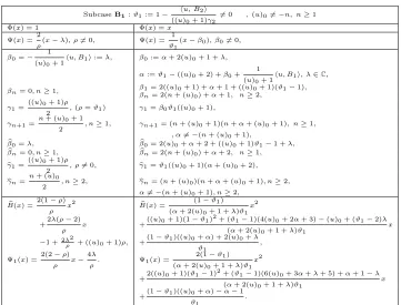
T a ble 1. The D u -Classical P olynomials -Case ( A ) Case ( A ): h u, B2 i = (( u )0 + 1) γ2 , ( u )0 6 = − n, n ≥ 1 A 1 : Φ( x ) = x 2 A 2 : Φ( x ) = x 2 − 1 β0 = ± 1 β0 6 = ± 1 Ψ( x ) = − 2( αx + 1) , Ψ( x ) = (( u )0 + 1)( x − β0 ) , Ψ( x ) = − σ ( x − β0 ) , σ 6 = 0 , β0 = − 1 α , α 6 = 0 , β0 = ± 1 , β0 6 = ± 1 , β1 = (( u )0 + 1)(( u )0 + 2) + 2 α 2θ α (( u )0 + 2)(( u )0 + 2 α + 1) , ( u )0 + 2 α + 1 6 = 0 , β1 ∈ C , β1 = σ θ − (( u )0 + 1)(( u )0 + 2) β0 (( u )0 + 2)(( u )0 + σ + 1) , σ 6 = − (( u )0 + 1) , βn = − (( u )0 + 2) θ (2 n + ( u )0 − 2)(2 n + ( u )0 ) , n ≥ 2 , βn = (( u )0 + 2) 2β 0 (2 n + ( u )0 − 2)(2 n + ( u )0 ) , n ≥ 2 , βn = − (( u )0 + 2) θ (2 n + ( u )0 )(2 n + ( u )0 − 2) , n ≥ 2 , γ1 = − (( u )0 + 1) α 2(( u )0 + 2 α + 1) , γ1 ∈ C \ { 0 } , γ1 − 2 β0 β1 − 2 6 = 0 , γ1 = (1 − β
2)((0
u )0 + 1) ( u )0 + σ + 1 , γ2 = − 2 αθ 2 (( u )0 + 2)(( u )0 + 3)(( u )0 + 2 α + 1) , θ 6 = 0 , γ2 = − (( u )0 + 2) γ1 − 2 β0 β1 − 2 ( u )0 + 3 , γ2 = σ (( u )0 + θ + 2)(( u )0 − θ + 2) (( u )0 + 2)(( u )0 + 3)(( u )0 + σ + 1) , θ 6 = ± (( u )0 + 2) , γn +1 = − ( n − 1)( n + ( u )0 + 1) θ 2 (2 n + ( u )0 − 1)(2 n + ( u )0 ) 2(2 n + ( u )0 + 1) , γn +1 = 4( n − 1) 2( n + ( u )0 + 1) 2 (2 n + ( u )0 − 1)(2 n + ( u )0 ) 2(2 n + ( u )0 + 1) , γn +1 = ( n − 1)( n + ( u )0 + 1)[(2 n + ( u )0 + θ )(2 n + ( u )0 − θ ) (2 n + ( u )0 − 1)(2 n + ( u )0 ) 2(2 n + ( u )0 + 1) , n ≥ 2 , n ≥ 2 , θ 6 = ± (2 n + ( u )0 ) , n ≥ 2 , bβ 0 = − (( u )0 + 1)( θ + 2) − 2 (( u )0 + 2)(( u )0 + 2 α + 1) , bβ 0 = 2 β0 + β1 , bβ 0 = (( u )0 + 2) σ β0 − (( u )0 + 1) θ (( u )0 + 2)(( u )0 + σ + 1) , bβ n = − ( u )0 θ (2 n + ( u )0 )(2 n + ( u )0 + 2) , n ≥ 1 , bβ n = ( u )0 (( u )0 + 2) β0 (2 n + ( u )0 )(2 n + ( u )0 + 2) , n ≥ 1 , bβ n = − (( u )0 + 2) θ (2 n + ( u )0 )(2 n + ( u )0 + 2) , n ≥ 1 , b γ1 = − (( u )0 + 1) θ 2 (( u )0 + 3)(( u )0 + 2) 2(( u )0 + 2 α + 1) , b γ1 = γ1 − 2 β0 β1 − 2 ( u )0 + 3 , b γ1 = (( u )0 + 1)(( u )0 + θ + 2)(( u )0 − θ + 2) (( u )0 + 2) 2(( u )0 + 3)(( u )0 + σ + 1) , b γn = − n ( n + ( u )0 ) θ 2 (2 n + ( u )0 − 1)(2 n + ( u )0 ) 2(2 n + ( u )0 + 1) , b γn = − 4( n − 1) n ( n + ( u )0 )( n + ( u )0 + 1) (2 n + ( u )0 − 1)(2 n + ( u )0 ) 2(2 n + ( u )0 + 1) , b γn = − ( n − 1)( n + ( u )0 )(2 n + ( u )0 + θ )(2 n + ( u )0 − θ ) (2 n + ( u )0 − 1)(2 n + ( u )0 ) 2(2 n + ( u )0 + 1) , , n ≥ 2 , n ≥ 2 , , n ≥ 2 , bB ( x ) = − α n α (( u )0 + 2 α + 1) x 2 bB ( x ) =
1 γ1
u
Case (B).
The subcase B1.Herehu, B2i= ((u)0+ 1)(1−ϑ1)γ2.The following system holds
(n+ (u)0+ 2)βbn−(n+ (u)0)βbn−1= (n+ (u)0+ 1)βn+1−(n+ (u)0−1)βn, n≥2.
(4.10) ((u)0+ 3)βb1−((u)0+ 1)βb0= ((u)0+ 2)β2−(u)0β1+hu, B1i. (4.11)
γn+2
n+ (u)0+ 2
− γn+1
n+ (u)0+ 1
= (βn+1−βbn)2, n≥1.
((u)0+ 1)ϑ1
(u)0+ 2 γ2−γ1= ((u)0+ 1)(β1−βb0)
2−(β
1−βb0)hu, B1i.
b
βn+1−βbn=βn+2−βn+1, n≥1. (4.12)
ϑ1βb1−βb0=ϑ1β2−β1+
1
(u)0+ 1hu, B1i. (4.13)
Using (4.12) in (4.10), we getβbn =−
1 2βn+2+
3
2βn+1, n≥1.Thus
βn = (β3−β2)(n−2) +β2, n≥2, so
b
βn=
(2n−3)
2 (β3−β2) +β2, n≥1. (4.14)
Thanks to (4.11), one has
b
β0=−
(u)0+ 3 2((u)0+ 1)
β3+
(u)0+ 5 2((u)0+ 1)
β2+
(u)0 (u)0+ 1
β1−
1 (u)0+ 1
hu, B1i, (4.15)
comparing (3.38) and (4.15), we obtain
−((u)0+ 2)((u)0+ 3)
2 β3+
((u)0+ 2)((u)0+ 5)
2 β2=β1+ ((u)0+ 1)β0+hu, B1i.
(4.16)
Thanks to (4.14), the relation (4.13) givesβ3=β2−
2c
ϑ1
,where
c= 1
(u)0+ 2
n
β0−β1+
1
(u)0+ 1hu, B1i
o
. (4.17)
Equation (4.16) becomes β2 = β1 +
c
ϑ1
h
((u)0 + 1)ϑ1 −((u)0 + 3)
i
. So β3 =
β1+
c
ϑ1
h
((u)0+ 1)ϑ1−((u)0+ 5)
i
, which gives βn = −
c
ϑ1
[2n+ (u)0−1]−c+
β0 +
1 (u)0+ 1
hu, B1i, n ≥ 2. From (4.17), we have β1 = −((u)0+ 2)c+β0+
1 (u)0+ 1
hu, B1i.Also, we haveβbn =−
c
ϑ1
h
2n+ (u)0
i
−c+β0+ 1 (u)0+ 1
hu, B1i, n≥
1.From (3.38), we obtainβb0=−((u)0+ 1)c+β0.Using the new expressions ofβn
andβbn,we get forn≥1:
γn+1=(((nu+()u)0+1)
0+1)ϑ1 n
γ1+c((u)0+ 1)
h
c− 1
(u)0+1hu, B1i
i
+ϑc2
1((u)0+ 1)(n−1) o
,
b
γn+1=(((nu+()u)0+1)
0+1)ϑ1 n
γ1+c((u)0+ 1)
h
c− 1
(u)0+1hu, B1i
i
+ϑc2
1((u)0+ 1)n o
,
b
γ1=γ1+ ((u)0+ 1)c
h
c− 1
(u)0+1hu, B1i
i
.
The system is completely solved. Note that in this case, deg Φ≤1 and
κΦ(x) =−((u)0+ 1)c
γ1
x+((u)0+ 1)cβ0
γ1
If deg(Φ) = 0 (c=0),then Φ(x) = 1.After a suitable affine transformation, we can
suppose that β0 =−
1 (u)0+ 1
hu, B1i := λ and γ1 =
((u)0+ 1)ρ
2 , where ρ :=ϑ1.
From (4.4) and (3.16), we get the expressions ofBb(x) and Ψ1(x).In particular, we
recognize here theD-Laguerre-Hahn sequence of class zero, nonsingular, of Hermite
type [2, 16] (see first column in Table 2).
If deg(Φ) = 1, (c 6= 0), then κ = −((u)0+ 1)c
γ1
, Φ(x) = x− γ1
((u)0+ 1)c
−β0
and Ψ(x) = −1
c(x−β0). By means of a suitable affine transformation, we can
chooseβ0andcsuch that
γ1
((u)0+ 1)c+β0= 0,andc=−ϑ1.Thus, Φ(x) =xand
Ψ(x) = 1
ϑ1
(x−β0).Puttingα=ϑ1−((u)0+ 2) +β0+ 1
(u)0+ 1hu, B1i,we get the expressions written in second column of Table 2.
In particular: Ifϑ1= 1,according to Proposition 3.7, the obtained sequence is the
D-Laguerre-Hahn sequence of class zero, nonsingular, of Laguerre type [2, 16]. If
ϑ16= 1,we recognize the perturbated sequence of order one of theD-Laguerre-Hahn
sequence of class zero, nonsingular, of Laguerre type [2, 16]. It is a D
-Laguerre-Hahn sequence of classs= 1.
Table 2. TheDu-Classical Polynomials -Case (B)
SubcaseB1:ϑ1:= 1−
hu, B2i
((u)0+ 1)γ2
6
= 0 ,(u)06=−n, n≥1
Φ(x) = 1 Φ(x) =x
Ψ(x) =2
ρ(x−λ), ρ6= 0, Ψ(x) =
1
ϑ1
(x−β0), β06= 0,
β0=−
1 (u)0+ 1
hu, B1i:=λ, β0:=α+ 2(u)0+ 1 +λ,
α:=ϑ1−((u)0+ 2) +β0+
1 (u)0+ 1
hu, B1i, λ∈C,
βn= 0, n≥1, ββ1= 2((u)0+ 1) +α+ 1 + ((u)0+ 1)(ϑ1−1), n= 2(n+ (u)0) +α+ 1, n≥2,
γ1=
((u)0+ 1)ρ
2 ,(ρ=ϑ1) γ1=β0ϑ1((u)0+ 1),
γn+1=
n+ (u)0+ 1
2 , n≥1, γn+1= (n+ (u)0+ 1)(n+α+ (u)0+ 1), n≥1,
, α6=−(n+ (u)0+ 1),
b
β0=λ, βb0= 2(u)0+α+ 2 + ((u)0+ 1)ϑ1−1 +λ,
b
βn= 0, n≥1, βbn= 2(n+ (u)0) +α+ 2, n≥1,
b
γ1=
((u)0+ 1)ρ
2 , ρ
6
= 0, bγ1=ϑ1((u)0+ 1)(α+ (u)0+ 2), b
γn=n+ (u)0
2 , n≥2, bγn= (n+ (u)0)(n+α+ (u)0+ 1), n≥2,
α6=−(n+ (u)0+ 1), n≥2,
b
B(x) =2(1−ρ)
ρ x
2
b
B(x) = (1−ϑ1)
(α+ 2(u)0+ 1 +λ)ϑ1
x2
+2λ(ρ−2)
ρ x +
((u)0+ 1)(1−ϑ1)2+ (ϑ1−1)(4(u)0+ 2α+ 3)−(u)0+ (ϑ1−2)λ
(α+ 2(u)0+ 1 +λ)ϑ1
x
−1 +2λ2
ρ + ((u)0+ 1)ρ, +
(1−ϑ1)((u)0+α) + 2(u)0+λ
ϑ1
,
Ψ1(x) =2(2−ρ)
ρ x−
4λ
ρ. Ψ1(x) =
2(1−ϑ1)
(α+ 2(u)0+ 1 +λ)ϑ1
x2
+2((u)0+ 1)(ϑ1−1)
2+ (ϑ
1−1)(6(u)0+ 3α+λ+ 5) +α+ 1−λ
(α+ 2(u)0+ 1 +λ)ϑ1
x
+(1−ϑ1)((u)0+α)−α−1
ϑ1
u
The subcase B2.Here κ=−
((u)0+ 1)ϑ1 (ρ+ 2)γ1
, and the polynomial Φ(x) is of degree
2 given by (4.8), where
(
d= 12
β0+β1+((u)ρ+2
0+2)ϑ1[β1−β0−
1
(u)0+1hu, B1i] ,
µ= 4(β0−d)2+ [((u()ρ+2)
0+1)ϑ1 + 1]γ1 .
(4.18)
As in the previous cases, we analyse the situations Φ(x) =x2,and Φ(x) =x2−1.
Particulary, we usually supposed= 0.Note that here Ψ(x) =−(ρ+ 2)
ϑ1
B1(x),and
b
B(x) = ((u)0+ 1)
γ1
nh
1−(ρ+ 1)ϑ1
ρ+ 2
i
x2+
h(ρ+ 1)ϑ
1
ρ+ 2 −1
i
(β0+β1) +
hu, B1i (u)0+ 1
x
(4.19)
+h1−(ρ+ 1)ϑ1
ρ+ 2
i
(β0β1−γ1) +
(u)0γ1 (u)0+ 1−
β0hu, B1i
(u)0+ 1
o
.
In particular, the sequence{Bn}n≥0is aD-Laguerre-Hahn sequence of classs≤2.
Besides, the system (3.41) becomes
(n+ (u)0+ 2)βbn−(n+ (u)0)βbn−1= (n+ (u)0+ 1)βn+1−(n+ (u)0−1)βn, n≥2.
(4.20) ((u)0+ 3)βb1−((u)0+ 1)βb0= ((u)0+ 2)β2−(u)0β1+hu, B1i. (4.21)
((u)0+ 2)βb0= ((u)0+ 1)β1+β0− hu, B1i. (4.22)
(2n+ (u)0+ρ+ 4) (n+ (u)0+ 2)(n+ρ+ 1)
γn+2−
(2n+ (u)0+ρ) (n+ (u)0+ 1)(n+ρ)
γn+1= (βn+1−βbn)2, n≥2.
(4.23) ((u)0+ρ+ 6)
((u)0+ 3)(ρ+ 2)
γ3−
h((u)0+ 1)ϑ1
ρ+ 2 + 1
i γ2
(u)0+ 2
= (β2−βb1)2. (4.24)
((u)0+ρ+ 4)
((u)0+ 2)(ρ+ 2)ϑ1γ2−
γ1
(u)0+ 1 = (β1−βb0)
β1−βb0−
1
(u)0+ 1hu, B1i
. (4.25)
(n+ρ+ 2)βbn+1−(n+ρ)βbn= (n+ρ+ 3)βn+2−(n+ρ+ 1)βn+1, n≥1. (4.26)
ϑ1βb1− 1−
ϑ1
ρ+ 2
b
β0=
(ρ+ 3)ϑ1
ρ+ 2 β2−β1+
1
(u)0+ 1hu, B1i. (4.27)
Subtracting (4.26) from (4.20), we get
((u)0−ρ+ 1)(βbn+1−βbn) = ((u)0−ρ−1)(βn+2−βn+1), n≥1. (4.28)
Two situations arise:
•B21: ρ6= (u)0−1
Hereβn+2−βn+1=ξ(βbn+1−βbn), n≥1,whereξ=
(u)0−ρ+ 1 (u)0−ρ−1.Then
βn+1=ξβbn+β2−ξβb1, n≥1.
Relation (4.20), wheren→n+ 1, gives
−(2n+ (u)0+ρ+ 5)
((u)0−ρ−1) βbn+1+
(2n+ (u)0+ρ+ 1)
(u)0−ρ−1 βbn= 2(β2−ξβb1), n≥1. (4.29)
On the other hand, sinced= 0,we have
hu, B1i= ((u)0+ 2)`−((u)0+ 1)
β0+ ((u)0+ 2)`+ ((u)0+ 1)
where`:=((u)0+1)ϑ1
ρ+2 .Then, (4.22) becomes
b
β0=−`β1+ (1−`)β0. (4.31)
Using (4.30) and (4.31), respectively in (4.21) and (4.27), gives
((u)0+ 3)βb1= ((u)0+ 2)β2+`β0+ (`+ 1)β1 (4.32)
(ρ+ 2)βb1= (ρ+ 3)β2+`β0+ (`+ 1)β1 (4.33)
The difference and the sum of the two last equations give respectively:
β2−ξβb1= 0, (4.34)
((u)0+ρ+ 5)(βb1−β2) = 2`β0+ 2(1 +`)β1. (4.35)
Therefore,
b
β1=−
((u)0−ρ−1)
(u)0+ρ+ 5 [`β0+ 2(1 +`)β1], (4.36)
β2=−
((u)0−ρ+ 1)
(u)0+ρ+ 5 [`β0+ 2(1 +`)β1]. (4.37)
Back to (4.29) and taking into account (4.34), we discuss two situations:
•B211: 2n+ (u)0+ρ+ 16= 0, ∀n≥1. Iterating (4.29) gives
( b
βn=−
((u)0+ρ+3)((u)0−ρ−1)[`β0+2(1+`)β1]
(2n+(u)0+ρ+1)(2n+(u)0+ρ+3) , n≥1,
βn+1=−
((u)0+ρ+3)((u)0−ρ+1)[`β0+2(1+`)β1]
(2n+(u)0+ρ+1)(2n+(u)0+ρ+3) , n≥1.
(4.38)
Therefore,
βn+1−βbn=−
2((u)0+ρ+ 3)[`β0+ 2(1 +`)β1] (2n+ (u)0+ρ+ 1)(2n+ (u)0+ρ+ 3)
, n≥1. (4.39)
In order to compute the coefficientsγn+1 andbγn+1,we study two possibilities:
•Φ(x) =x2.Takingµ= 0 and using (4.30) in (4.18), we haveβ2
0+γ1(1 +
1
`) = 0.
Besides, from (4.31) and (4.30) one has
(
β1−βb0= (`−1)β0+ (`+ 1)β1,
β1−βb0−(u)1
0+1hu, B1i= −`
(u)0+1(β0+β1).
(4.40)
Necessarily 1 +1` 6= 0.Otherwiseβ0= 0.Then, from (4.31) we obtainβb0−β1= 0. Therefore, equation (4.35) leads toβb1−β2= 0.Then (4.24) gives (u)0+ρ+ 6 = 0.
Takingn= 3 in (4.23), givesγ5= 0 which is absurd. We conclude that
γ1=
−`β2 0
1 +`, β06= 0. (4.41)
In (4.25), necessarily (u)0+ρ+ 46= 0.If not, one hasγ1=−((u)0+ 1)(β1−βb0) β1−
b
β0−(u)10+1hu, B1i
. Thanks to (4.40) and (4.41), we get `β0+ (1 +`)β1
2
= 0,
or equivalently`β0+ (1 +`)β1 = 0.Thus, (4.35) proves that βb1−β2 = 0.Taking
into account (4.34), we deduceβb1=β2= 0.So, from (4.39) we obtainβn+1−βbn=
0, n≥1.Equation (4.23), wheren= 2, implies thatγ4= 0 which is not possible.
Once the expression ofγ2 is obtained, we easily deduce the rest of the three term
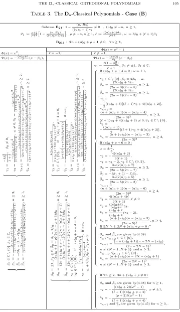
recurrence coefficients (see first column in Table 3). In addition, we have
b
B(x) =−1+`
`β2 0
n
u
((u)0+ρ+ 3)`−2((u)0+ 1)
β0+ ((u)0+ρ+ 3)`β1
x+
(u)0+ 1−(ρ+ 1)`
β0β1−
`β02[(ρ+1)`−1]
1+`
o
.
Ψ1(x) =−1+` `β2 0
n
(u)0+ 1−(ρ+ 1)`x3+
((u)0+ 2)`−((u)0+ 1)β0+ ((u)0+ρ+ 3)`β1 x2+
((u)0+ρ+ 3)`−2((u)0+ 1)
β20+
(u)0+ 1 + ((u)0+ 2)`
β0β1−
β20[(ρ+1)`2−`−(u)0−1]
1+` x
+
(u)0+ 1−(ρ+ 1)`
β2 0β1−
β03[(ρ+1)`2−`−(u)0−1]
1+`
o
.
•Φ(x) =x2−1.We note here that since too many subcases will appear later, we
simply refer to (4.19) and (3.16) for computing the polynomialsBb(x) and Ψ1(x).On
the other hand, takingµ= 4 and using (4.30) in (4.18), we getγ1(1 +1`) = 1−β02.
We distinguish two subcases:
If ` =−1, relations (4.30), (4.31) and (4.40) are still valid. Besides, β0 = ±1
andγ1∈C\ {0}.Thus, it is easy to obtain the corresponding coefficients given in
the second column of Table 3.
If`6=−1,we have γ1=
`(1−β02)
`+ 1 , β06=±1 and relations (4.30), (4.31), (4.35)
and (4.40). In order to explicit the coefficientsγn andbγn,we need to discus many
situations when solving equations (4.23)-(4.25). The results are summarized in the last column of Table 3.
•B212: ∃N ≥1,such that 2N+ (u)0+ρ+ 1 = 0.From (4.34), we get
(N+ (u)0+ 1)βb1−(N+ (u)0)β2= 0. (4.42)
Therefore, subtracting (4.20) from (4.26), we obtainβbn=
N+ (u)0
N+ (u)0+ 1βn+1, n≥1.
Then, from (4.20) we have (n−N+ 2)βn+2−(n−N)βn+1 = 0, n≥1.Thus, the
expressions ofβn andβbn hold as shown in Table 4.
For N ≥3, we have β2 = 0. Thanks to (4.42), one has βb1 = 0. Consequently,
taking into account (4.30), (4.31) and (4.32), we get
b
β0=β0+β1, β0= (1 +`)βb0, β1=−`βb0, β1−βb0=−β0,
hu, B1i=−[(u)0`+ (u)0+ 1]βb0,
β1−βb0−(u)1
0+1hu, B1i=−
`
(u)0+1βb0,
(4.43)
where`=− ((u)0+ 1)ϑ1
2N+ (u)0−1.The coefficientsγn+1 satisfy the following system:
(2n−2N+3)
(n+(u)0+2)(n−2N−(u)0)γn+2−
(2n−2N−1)
(n+(u)0+1)(n−2N−(u)0−1)γn+1= 0,
where n≥2, n6∈ {N−1, N}, 1
(N+(u)0+1)2γN+1+
3
(N+(u)0+1)(N+(u)0+2)γN =
−β2 N
(N+(u)0+1)2,
3
(N+(u)0+2)(N+(u)0)γN+2+
1
(N+(u)0+1)2γN+1=
−β2N
(N+(u)0+1)2,
(2N−5)
((u)0+3)(2N+(u)0−1)γ3−
1+`
(u)0+2γ2= 0,
(2N−3)`
(u)0+2 γ2+γ1=−(1 +`)`βb
2
0.
Remark that `6=−1, otherwise we obtain γ3= 0.If we assume that µ= 0, then
thanks to (4.18) this is equivalent to γ1 =−
β2 0
1+`. So γ2 = 0 which is impossible.
We conclude that necessarily µ= 4, or equivalentlyγ1=
`(1−β2 0)
1+` .The coefficients