Multi-Objective Gene Expression Programming for Clustering

Multi-Objective Gene Expression Programming for Clustering

Yifei Zheng, Lixin Jia, Hui Cao



State Key Laboratory of Electrical Insulation and Power Equipment, Electrical Engineering School Xi'an Jiao Tong University, Shaanxi Province, 710049, China

Email: [email protected], {lxjia, huicao}@mail.xjtu.edu.cn

http://dx.doi.org/10.5755/j01.itc.41.3.1330

Abstract. This paper proposes a multi-objective gene expression programming for clustering (MGEPC), which

could automatically determine the number of clusters and the appropriate partitioning from the data set. The clustering algebraic operations of gene expression programming are extended first. Then based on the framework of the Non-dominated Sorting Genetic Algorithm-II, two enhancements are proposed in MGEPC. First, a multi-objective k-means clustering is proposed for local search, where the total symmetrical compactness and the cluster connectivity are used as two complementary objectives and the point symmetry based distance is adopted as the distance metric. Second, the power-law distribution based selection strategy is proposed for the parent population generation. In addition, the external archive and the archive truncation are used to keep a historical record of the non-dominated solutions found along the search process. Experiments are performed on five artificial and three real-life data sets. Results show that the proposed algorithm outperforms the PESA-II based clustering method (MOCK), the archived multiobjective simulated annealing based clustering technique with point symmetry based distance (VAMOSA) and the single-objective version of gene expression programming based clustering technique (GEP-Cluster).

Keywords: Clustering; multi-objective; evolutionary algorithm; gene expression programming.

 Corresponding author

1. Introduction

Clustering is the assignment of a set of unlabeled objects into groups such that objects from the same group are more similar to each other than objects from different groups. Clustering algorithms have been widely applied into many different fields, such as image processing [6], text categorization [19], market segmentation [14], eye gaze visualizations [20], etc. Since clustering could be considered as a particular kind of optimization problem, evolutionary algorithms have been proposed for clustering [11].

Gene Expression Programming (GEP), which combines the advantages of both genetic algorithm and genetic programming, is a relatively new member in the evolutionary computation family [8]. GEP works with two entities called the chromosome and the expression tree. The separation of the chromosome and the expression tree ensures that expression trees are always syntactically correct after any genetic change of chromosomes; thus the exploration of the search space is greatly expanded. Therefore, GEP shows powerful capabilities over a large variety of domains, including regression modeling, optimization, classification tasks and time series prediction [9, 22, 12, 23].

A clustering technique based on GEP (GEP-Cluster) was first proposed in [4], and a new concept named the clustering algebra, which performs clustering as algebraic operation, is presented. GEP-Cluster could divide or merge the clusters automatically without any prior knowledge. However, like the conventional evolutionary clustering algorithms performing with just one clustering criterion, GEP-Cluster is also a single-objective clustering method. For a wide variety of real life datasets, a single clustering criterion is hardly able to judge the correctness of clustering result. Furthermore, since there would be considerable discrepancies between solutions produced by the same algorithm using different clustering criteria, an inappropriate choice of the validity measure may lead to poor clustering results [21]. Therefore, for overcoming the limitation of single-objective clustering method, the concept of multi-objective clustering has been introduced [3, 10, 13, 16, 18].

avoiding using a huge amount of computational resources to edit those illegal chromosomes. Then based on the framework of the Non-dominated Sorting Genetic Algorithm-II (NSGA-II), two enhancements are proposed in MGEPC. First, a multi-objective k-means method is presented as a local search, which performs fine-tuning of some rough partitions obtained by the global search, to speed up the convergence. Second, the power-law distribution based selection strategy is proposed for ensuring some inferior individuals being selected into the next generation while maintaining a bias against superior solutions, which helps maintain the diversity of the population and avoids getting stuck at a local optimal or partial Pareto front. In addition, the external archive and the archive truncation are used to keep a historical record of the non-dominated solutions found along the search process.

The remainder of the paper is organized as follows: Section 2 reviews relevant previous work. In Section 3, the proposed algorithm is discussed in detail. Section 4 shows the experimental setup and comparison results on both artificial and real-life data sets. Finally, Section 5 concludes the paper.

2. Related works

MOCK is a popular multi-objective evolutionary clustering algorithm based on PESA-II (PESA-II is a multiobjective evolutionary algorithm proposed in [5]). It optimizes two complementary objectives, which are the cluster compactness and the connectedness [10]. It has been shown to outperform traditional single-objective clustering techniques across a diverse range of benchmark data sets. However, since MOCK employs a locus-based adjacency encoding scheme, namely, the length of each chromosome is equal to the number of points present in the data set; the length of each chromosome would increase with the number of points. Hence, MOCK would suffer from premature convergence for long chromosomes in large search space [15].

VAMOSA, which is an archived multiobjective simulated annealing based clustering technique with point symmetry based distance, adopts a variable-length real encoding, namely, the strings are made up of real numbers which represent the coordinates of the centers of partitions [16]. Therefore, for data sets of large cluster numbers and high dimensions, VAMOSA has the same drawback as MOCK. Moreover, since the mutation mechanism could only add or remove one cluster center at a time, the exploration of the search space would be limited to a certain extent. Thus VAMOSA suffers from a slow convergence rate and often easily falls into local optimality.

GEP-Cluster is a GEP-based clustering method without prior knowledge. It introduces a new encoding scheme based on clustering algebraic operations [4]. Although GEP-Cluster could overcome the limitation in the representation of MOCK and VAMOSA, a large

number of invalid chromosomes would appear in the evolving process of GEP-Cluster and a huge amount of computational resources would be wasted. In addition, GEP-Cluster chooses the overall deviation as the objective. Since the overall deviation would increase with the number of clusters increasing, the number of clusters detected by the iteration process would always be the maximum cluster number pre-specified. Although GEP-Cluster employs an automatic merging cluster algorithm to adjust clusters after the iteration process, it is effective only when true clusters in the data set are well-separated.

In the next section, we will present a new clustering algorithm named MGEPC. In Section 4, we will use artificial and real-life datasets to compare the effectiveness of MGEPC with that of MOCK, VAMOSA and GEP-Cluster, respectively.

3. The Proposed Method

3.1. Multiobjective optimization

We consider the clustering task as a multiobjective optimization problem (MOP), which can be mathematically formulated as [24]

Minimize ( ) ( ₁( ), , ( )T)

m x

f x f x

F  _ , s.t. x (1)

where  is the decision space and x is a decision vector. F x( ) consists of m objective functions f ii, 1,...,m.

The objectives of MOP often conflict with each other. Improvement of one objective may lead to deterioration of another. Thus there no longer exists a single optimal solution but rather a set of trade-off solutions, which is called the Pareto optimal solutions. Some definitions related to the Pareto optimality are given as follows.

Definition 1 (Pareto dominance). A solution xp is said to dominate another solution xq (denoted by

p q

x _x ), if and only if  k 1,...,m, f x( )p  f x( )q and  k 1,...,m, f x( )p  f x( )q .

Definition 2 (Pareto-optimal set). If no solution dominates xp , then xp is a Pareto-optimal solution. The set of all feasible Pareto-optimal solutions is called Pareto-optimal set.

Definition 3 (Pareto front). The image of Pareto-optimal set in the objective space is called the Pareto front.

3.2. Representation

3.2.1. Clustering algebraic operations

Clustering operators used in GEP-Cluster are ‘



’ and ‘



’ [4]. Let Ox be the center of cluster Cx, and

y

O be the center of cluster Cy. Then

(1) OxOy {Oxy}, where Oxy is the mean point of

x

O and Oy.

(2) OxOy { ,O Ox y}.

The first operation indicates that Cx and Cy are merged into one cluster with the center Oxy, and the

second operation indicates that Cx and Cy would not be merged together, namely, they are two separate clusters with the center Ox and Oy.

Based on the concepts of the clustering operators, we extend the clustering algebraic operations, which are presented in Theorem 1.

Theorem 1: Let O , x Oy and O be the centers of z cluster C , x Cy and C in the d-dimensional space, z and Ox ( , ,..., )x x1 2 xd , Oy ( , ,...,y y1 2 yd) ,

1 2 ( , ,..., )

z d

O  z z z , then

(1) OxOyOyOx; OxOy OyOx

(2) _{( ) {(}2 1 1 1_,2 2 2 2_,...,2 _)}

4 4 4

d d d

x y z

x y z x y z x y z

O  O O        ;

1 1 2 1 2 2 2 2 2

( ) {( , ,..., )}

4 4 4

d d d

x y z

x y z x y z x y z

O O O       

(3) Ox(OyOz) ( OxOy)Oz {( , ,..., ),( , ,...,x x1 2 xd y y1 2 yd),( , ,..., )}z z1 2 zd

(4) 1 1 2 2

1 2

( ) {( , ,..., ),( , ,..., )}

2 2 2

d d

x y z d

y z y z y z

O  O O  x x x   

(5) )}

2 ,..., 2 , 2 ( ), 2 ,..., 2 , 2 {( )

( 1 1 2 2 d d 1 1 2 2 d d

z y x z x z x z x y x y x y x O O

O         

▼Proof:

(1)This commutative law has been proved in [4].

(2)The operation Ox(OyOz) indicates that Cy and Cz are merged into cluster yz

C _{with the center}

1 1 2 2

( , ,..., )

2 2 2

d d yz

y z y z y z

O     , and then Cyz

and Cx are merged into cluster xyz

C _{with the center}

1 1 1 2 2 2

2 2 2

( , ,..., )

4 4 4

d d d

xyz

x y z x y z x y z

O        .

Similarly, the operation (OxOy)Oz indicates that Cx, y

C _and z

C are ultimately merged into one

cluster with the center

1 1 2 1 2 2 2 2 2

( , ,..., )

4 4 4

d d d

x  y z x y  z x y  z _.

Consequently, operator ‘  ’ is not always associative.

(3)The operation Ox(OyOz) indicates that Cy and Cz are separate clusters, and Cx is separate from Cy and Cz. Thus Cx, Cy and Cz are three distinct clusters with the center Ox, Oy and Oz, respectively. Similarly, (OxOy)Oz also indicates that Cx, Cy and Cz are three distinct

clusters. Therefore, the equation

( ) ( )

x y z x y z

O  O O  O O O is satisfied, and

the three cluster centers are ( , ,..., )x x1 2 xd ,

1 2

( , ,...,y y yd) and ( , ,..., )z z1 2 zd respectively.

(4)The formula Ox(OyOz) _{indicates that} Cy and Cz are merged into cluster yz

C _{with the center}

yz

O _{, and then} Cyz _and x

C are kept separate. That is to say, there are two clusters with thecenters Ox

and Oyz _{, namely,} ( , ,..., )x x1 2 xd _and 1 1 2 2

( , ,..., )

2 2 2

d d y z y z y z

.

(5)The operation Ox(OyOz) indicates that Cx will be merged with Cy and Cz respectively. Thus the merged cluster centers are

1 1 2 2

( , ,..., )

2 2 2

d d x y x y x y

and

1 1 2 2

( , ,..., )

2 2 2

d d x z x z x z _.▲

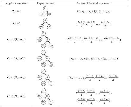
Table 1. The clustering algebraic operations, the corresponding expression trees and the centers of the resultant clusters

Algebraic operation Expression tree Centers of the resultant clusters

x y

O O ( , ,..., )x x1 2 xd ( , ,...,y y1 2 yd)

x y

O O ( 1 1, 2 2,..., )

2 2 2

d d x y x y x y

( )

x y z

O  O O (2 1 1 1,2 2 2 2,...,2 )

4 4 4

d d d

x  y z x y z x y z

( )

x y z

O  O O ( , ,..., ),( , ,...,x x1 2 xd y y1 2 yd),( , ,..., )z z1 2 zd

( )

x y z

O  O O ( , ,..., ),(_{1 2} 1 1, 2 2,..., )

2 2 2

d d d

y z y z y z

x x x   

( )

x y z

O  O O

1 1 2 2

( , ,..., )

2 2 2

d d x y x y x y _,

1 1 2 2

( , ,..., )

2 2 2

d d x z x z x z

.

3.2.2. Encoding

Each chromosome of MGEPC is composed of a head and a tail. The head contains symbols that represent both the functions (the elements from the function set F) and terminals (the elements from the terminal set T), whereas the tail contains only terminals. The function set F is {



,



}, and the terminal set T is {1, 2, …, i, …N}, i[1, ]N , where N is the number of data points in the data set and i is the sequence number of the ith data point. The first position in the head should always be set as ‘



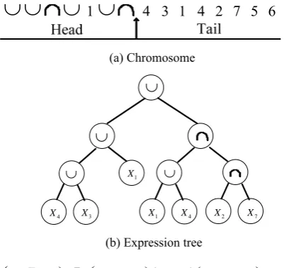
’ in order to ensure the clustering problem meaningful. Other positions in the head are set as a randomly selected function or a randomly selected terminal based on an equal probability. Elements in the tail are chosen from the terminal set randomly. Duplicate terminals are allowed in the chromosome because the information encoded in the chromosome is cluster centers rather than link of each data item.Let h denote the length of the head and t denote the length of the tail. Since the maximum arity of the clustering operators is 2, then t h 1 [8]. It is evident from the clustering expression tree that a chromosome could express h1 clusters at most. Thus, if the maximum

number of clusters is kmax, the total length of the chromosome mht(kmax1)((kmax1)1)

1 2 max

 k . Figure 1 gives an example of the

representation of a chromosome for MGEPC, where i

X ( =1,2,...,7i ) indicates the ith data point. Figure 1 (a) showsa chromosome of MGEPC. Figure 1 (b) and Figure 1 (c) show its corresponding expression tree and clustering algebraic operation, respectively.

3.2.3. Decoding

The translation from the chromosome to the expression tree is performed by a breadth-first traversal from left to right and from top to down [8]. The algebraic operation is obtained by a traversal in the reverse order, and the resultant cluster centers are evaluated according to Table 1.

Because the number of the nodes of an expression tree is m at most, the translation from the chromosome to the expression tree requires at most O m( ) time. Evaluation of expression tree also requires at most

( )

O m time. Therefore, this decoding step requires at

 

1



4 3 1 4 2 7 5 6

(a) Chromosome

(b) Expression tree

1

X X4

2

X X7



)



( X4



X3



X1)

(c) Clustering algebraic operation

Figure 1. An example of the representation of a

chromosome for MGEPC

This representation has two advantages. First, clusters could be merged or kept separate automatically by clustering operations. Thus there is no need to pre-specify the number of clusters, which is usually difficult to estimate in many applications. Second, extension of the clustering algebraic operations not only avoids using a huge amount of computational resources to edit those illegal chromosomes in the evolving process, but also allows modification of the chromosome using nearly any genetic operator without restrictions; thus the exploration of the search space is greatly enhanced.

3.3. Point symmetry based distance measure Since symmetry is a basic feature of most shapes and objects, it can be considered as an important feature in their recognition and reconstruction. Symmetry is a natural phenomenon and clusters are not exception. Based on this observation, a point symmetry based distance (PS distance) is developed in [2]. Then assignment of points to different clusters is done based on the PS distance rather than the Euclidean distance. This enables the clustering algorithm to automatically evolve clusters of any shape, size or convexity as long as they possess some symmetry property.

The PS distance proposed in [2] is defined by

1 2

( , ) ( ) / 2 ( , )

ps i k e i k

d x c  d d d x c (2)

where d x ce( , )i k is the Euclidean distance between the point xi and the cluster center ck . d1 and d2 are distances of the two nearest neighbors of the symmetrical point (i.e. 2 ck xi) of xi with respect

to the center ck. To reduce the complexity of finding

1

d and d2, an ANN search using the Kd-tree method is used.

3.4. Objective functions

The objective functions corresponding to a state indicate the degree of goodness of the solution it represents. In this paper, two complementary objectives that reflect fundamentally different aspects of a clustering solution are selected: one is the total symmetrical compactness; the other is the cluster connectivity.

The total symmetrical compactness measures the within cluster total symmetrical distance. It is computed as the overall summed PS distance between data objects and their corresponding cluster center. It is defined as [17]

1 1 1

( , )

i n

k k

i

k i ps j i

i i i

E

d

x c



  









₍₃₎

where k is the number of clusters, ni is the total

number of points present in the ith cluster, ci is the

center of the ith cluster, and xij is the jth point of

the i th cluster. ( , )i

ps j i

d x c denotes the PS distance between i

j

x and ci . Ei is the total symmetrical

deviation of a particular cluster i. Note that when the partitioning is compact and has good symmetrical structure, k should be low. Thus for achieving better

partitioning, the total symmetrical compactness should be minimized.

The cluster connectivity evaluates the degree to which neighboring data points have been placed in the same cluster. It is calculated as [10]

, 1 1

( )

(

ij

)

N L

i n

i j

Conn c

x

 



 

(4)

where , 1

, :

0,

ij

k i k ij k

i n

if C x C n C

j x

otherwise

 _{   }

  

 ,

ij

n is the jth nearest neighbor of the i th datum, N is the size of the data set, and L is a parameter

determining the number of neighbors that contribute to the connectedness. As an objective of clustering, the cluster connectivity should be minimized.

The objective value associated with the total symmetrical compactness necessarily improves with an increasing number of clusters, and the opposite is the case for the cluster connectivity. Thus the interaction of these two objectives allows MGEPC to automatically determine the number of clusters and generate clustering solutions corresponding to different trade-offs.

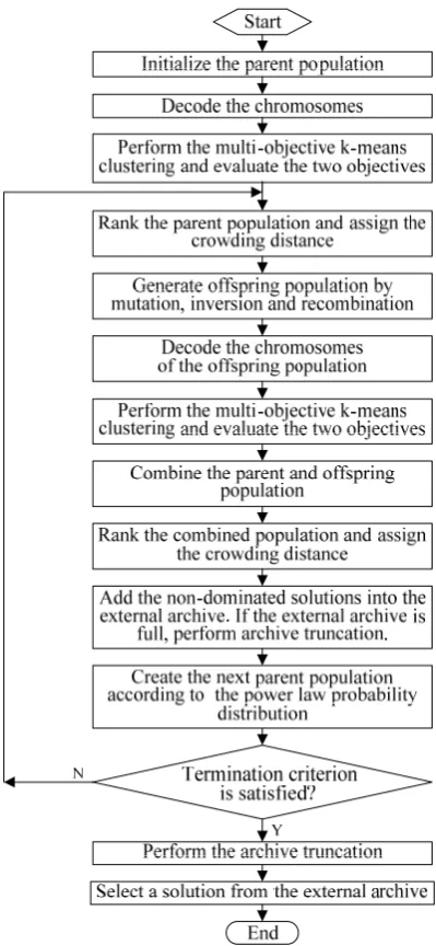
3.5. Description of the algorithm

In the subsection, MGEPC is formulated in detail. The flowchart of the MGEPC is shown in Figure.2 first, and the outline of MGEPC is presented in the following.



 

4

X X3 X1 X4 X2 X7



1

Figure 2. Flowchart of the MGEPC

Procedure MGEPC

Input: the data set D, the population size NP , the maximum number of generations Gmax , the maximum number of clusters kmax, the number of neighbors that contribute to the connectedness L ,

mutation rate pM, inversion rate pI, recombination rate pR, the parameter of power law distribution  , the maximum number of loops of multiobjective k-means clustering Liter and the external archive size

A N .

Output: the cluster label of each data point. Step 1: Initialize the parent population.

Step 2: Decode the chromosomes. Then the multi-objective k-means clustering is performed as follows: Assign each point to one of the clusters according to the point assignment method proposed in [2], which is shown in Figure 3. After the assignments are finished, two objective functions are evaluated and

the cluster centers are replaced by the mean points of the respective clusters. This process is repeated until the maximum number of iterations is reached or the value of any objective function becomes larger than that computed in the last loop. Finally, output the objective values of each chromosome. Since the multi-objective k-means clustering works as a local search to refine the global search performed by the evolutionary procedure, the convergence is speeded up.

Procedure: assignment of data points

1. Let K denote the number of clusters encoded in one of the chromosomes. For all data points xi, 1≤i≤N,

compute

) , ( min

arg _{1, ,} *

k i ps K

k d x c

k  _

2. If dps(xi,ck*)/de(xi,c_k*) , where



is the maximum nearest neighbor distance among all the points in the data set, assign the data point x_i to the k*th

cluster.

3. Otherwise the data point x_i is assigned to the k*th

cluster, where

) , ( min

arg 1, , *

k i ps K

k d x c

k  _

Figure 3. Data point assignment procedure

Step 3: Rank the population based on the non-dominated sorting and assign the crowding distance in each front. These two operations are proposed in [7] and are used for population selection. The non-dominated sorting is to rank each individual based on the definition of domination. Specifically, individuals not dominated by any other individuals are assigned front number 1, and individuals only dominated by individuals in front number 1 are assigned front number 2, and so on. The crowding distance is used to measure the density of individuals with the same front number. The crowding distance of a particular individual is computed as the average distance of two closest individuals on either side of this individual along each of objectives.

the root, and inverts the element order in the fragment. Since the inversion operator is restricted to the head of the chromosome, all the new individuals created by inversion are syntactically correct. (3) Recombination: the recombination operator exchanges parts of a pair of randomly chosen chromosomes to form new offspring chromosomes. In this paper, one-point recombination is used.

Step 5: Decode the chromosomes of the offspring population and perform the multi-objective k-means clustering.

Step 6: Combine the parent and offspring population. Then rank the combined population based on non-dominated sorting and assign the crowding distance in each front.

Step 7: Add the non-dominated solutions into the external archive. We set the upper limit of the size of the external archive as NA (NA is a much larger number than the population size NP ) in order to prevent the elitists from growing extremely large. If the size of the external archive exceeds the upper limit, archive truncation is performed as follows: the non-dominated solutions in the external archive are identified firstly. Then the dominated solutions are discarded. If the size of non-dominated solutions is still larger than NA, only NA solutions with higher value of crowding distance are retained in the external archive.

Step 8: Create the next parent population from the combined population according to the power law probability distribution. This process has two substeps: a front is selected by a power law probability P u( )1 u1 firstly, where u1 is the front number sorted based on the non-domination,  is a user specified parameter. Then a solution is chosen from the selected front by P u( )2 u2, where u2 is the sequence number of solutions sorted by decreasing the crowding distance and the solutions are selected without replacement. For 0, it is exactly a random selection. For    , it approaches the elitist-preserving process as in NSGA-II. For a given value of  , the selection ensures that no front and no crowded regions get completely excluded from further evolution while the evolution maintains a biastowards superior solutions. Hence, the power-law distribution based selection strategy for new parent population could not only keep a high convergence rate, but also maintain the diversity in the population, which would prevent the algorithm from getting stuck at a local optimal or partial Pareto front.

Step 9: Go to Step 3 if termination criterion is not satisfied, otherwise go to Step10.

Step 10: Perform the archive truncation and output solutions in the external archive. The output of the external archive contains a number of mutually non-dominated clustering solutions, which correspond

to different tradeoffs between the two objectives, and also to different numbers of clusters.

Step 11: Select a solution from the external archive, where we use the model selection method proposed in MOCK to select the most promising clustering solution.

Step 12: Output the clustering result.

By the proposed algorithm, the clustering for the data set is finished and the number of clusters is determined automatically. In the next section, we will use the experimental results to verify the effectiveness of the proposed algorithm.

4. Experimental results

In this section, we present experiments on artificial and real-life datasets to evaluate the performance of the proposed MGEPC. The algorithm is compared with MOCK, VAMOSA and GEP-Cluster based on two widely used clustering quality evaluation measures: the adjusted rand index (ARI) [10] and the Minkowski score (MS) [16]. The higher the value of ARI and the lower the value of MS, the better the clustering quality is. Experiments are implemented in MATLAB 2009a and the running environment is an Intel (R) CPU 2.50 GHz machine with 3 GB of RAM and running Windows XP Professional.

4.1. Data sets

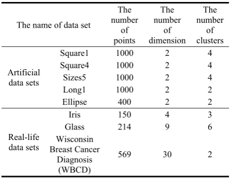
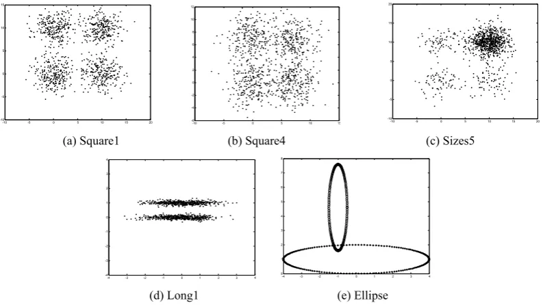
Five artificial data sets and three real-life data sets are used for the experiment. A short description of the data sets in terms of the number of data points, dimension and the number of clusters is provided in Table 2. The artificial data sets are displayed in Figure 4. Square1 [10] contains four well-separated squared clusters. Square4 [10] contains four overlapping squared clusters. Sizes5 [10] contains clusters of non-uniform densities. Long1 [10] contains two long-shaped clusters. Ellipse [2] contains data points distributed on two crossed ellipsoidal shells. The three real-life datasets are obtained from the UCI Machine Learning Repository [1].

Table 2. Details of the datasets used

The name of data set

The number

of points

The number

of dimension

The number

of clusters

Artificial data sets

Square1 1000 2 4

Square4 1000 2 4

Sizes5 1000 2 4 Long1 1000 2 2 Ellipse 400 2 2

Real-life data sets

Iris 150 4 3 Glass 214 9 6 Wisconsin

Breast Cancer Diagnosis

(WBCD)

(a) Square1 (b) Square4 (c) Sizes5

(d) Long1 (e) Ellipse

Figure 4. Artificial data sets

4.2. Parameters of the algorithms

In this subsection, we list the specification of parameters for the four algorithms. For MGEPC, the population size NP50, the maximum number of generations Gmax 100 , the external archive size

1000

A

N  , the maximum number of clusters kmax=

= N _{(N denotes the size of the data set), the number}

of neighbors that contribute to the connectedness 10%

L N , the recombination rate pR 0.7 , the mutation rate pM 0.1, the inversion rate pI 0.1, the parameter of power law distribution 1.4 and the maximum number of loops of multi-objective k-means clustering Liter 3. These parameter values are recommended for MGEPC after performing a great number of hand-tuning experiments. For MOCK, the population size is 50, the number of generations is 100, the maximum number of clusters is N , the

number of neighbors that contribute to the connectedness L is 10%N, the recombination rate is 0.7 and the mutation rate is 0.1. For VAMOSA, in order to make direct comparisons possible, we set the maximum temperature Tmax 100 , the minimal

temperature 8

min 2 10

T    , the cooling rate 0.8 and the number of iterations at each temperature

50

iter so that it has approximately the same number of function evaluations with the other three algorithms. For GEP-Cluster, the population size is 50, the number of generations is 100, the maximum number of clusters is N, the recombination rate is

0.7 and the mutation rate is 0.1.

4.3. Experimental results

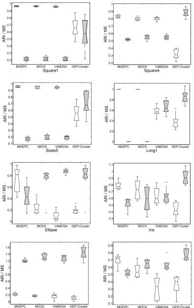
The mean values and standard deviations of the number of clusters, ARI and MS values for the eight data sets over 30 consecutive runs for MGEPC, MOCK, VAMOSA and GEP-Cluster are provided in Table 3. The distributions of ARI values and MS values are also visualized in Figure 5. It can be seen that MGEPC, MOCK and VAMOSA, which are the multi-objective clustering methods, consistently outperform GEP-Cluster algorithm in terms of the cluster numbers detected, ARI and MS values. For Square1, Square4 and Sizes5 which are composed of spherically-shaped clusters, MGEPC, MOCK and VAMOSA are always able to detect the appropriate number of clusters; and MGEPC performs better than MOCK and VAMOSA. The results of Square4 show that MGEPC performs well for overlapping clusters, and the results of Sizes5 show that MGEPC is also able to detect clusters of different densities and sizes. For Long1, both MGEPC and MOCK could detect the right partitions. For Ellipse, only MGEPC could detect the right number of clusters, and the mean values of ARI and MS are much better than those of MOCK and VAMOSA while their standard deviations are higher. The results of Long1 and Ellipse show that MGEPC is able to detect the appropriate partitioning from data sets with non-hyperspherical clusters as long as they possess the property of symmetry. For Iris, WDBC and Glass, MGEPC performs better than the others. Therefore, the effectiveness of MGEPC for clustering is higher.

-10 -5 0 5 10 15 20 -10

-5 0 5 10 15

-10 -5 0 5 10 15 -6

-4 -2 0 2 4 6 8 10 12

-10 -5 0 5 10 15 20 -10

-5 0 5 10 15 20

-4 -3 -2 -1 0 1 2 3 4 -4

-3 -2 -1 0 1 2 3 4

-4 -3 -2 -1 0 1 2 3 4 0

Table 3. Mean values and standard deviations (in parentheses) of number of clusters, ARI and MS for different data sets over 30

consecutive runs of different algorithms

Data set Real number of _clusters Algorithm k ARI MS

Square1 4

MGEPC 4 (0) 0.9686 (0.0076) 0.1995 (0.0268)

MOCK 4 (0) 0.9614 (0.0096) 0.2183 (0.0324)

VAMOSA 4 (0) 0.9672 (0.0118) 0.2123 (0.0251)

GEP-Cluster 5.42 (0.93) 0.6254 (0.1419) 0.5749 (0.2256)

Square4 4

MGEPC 4 (0) 0.8305 (0.0192) 0.5197 (0.0146)

MOCK 4 (0) 0.7991 (0.0247) 0.5477 (0.0348)

VAMOSA 4 (0) 0.8036 (0.0265) 0.5310 (0.0291)

GEP-Cluster 3.50 (1.24） 03165 (0.2723) 0.8910 (0.2647)

Sizes5 4

MGEPC 4 (0) 0.9593 (0.0176) 0.1821 (0.0293)

MOCK 4 (0) 0.9469 (0.0178) 0.1940 (0.0339)

VAMOSA 4 (0) 0.9507 (0.0161) 0.1931 (0.0375)

GEP-Cluster 3.48 (0.83) 0.5593 (0.1454) 0.6981 (0.1852)

Long1 2

MGEPC 2 (0) 1 (0) 0 (0)

MOCK 2 (0) 1 (0) 0 (0)

VAMOSA 1.58 (0.62) 0.5843 (0.0936) 0.6774 (0.1321) GEP-Cluster 3.72 (0.42) 0.3810 (0.1320) 0.8762 (0.1566)

Ellipse 2

MGEPC 2 (0) 0.7385 (0.2472) 0.4433 (0.2701)

MOCK 7.8 (0.31) 0.2357 (0.1041) 0.7387 (02092) VAMOSA 4.75 (0.83) 0.2221 (0.1134) 0.7116 (0.2287) GEP-Cluster 6.4 (0.79) 0.1954 (0.2569) 1.9766 (0.3743)

Iris 3

MGEPC 3 (0) 0.7944 (0.0529) 0.4831 (0.0740)

MOCK 3.05 (0.15) 0.7287 (0.1382) 0.5944 (0.1827) VAMOSA 3.87 (0.99) 0.3105 (0.1633) 0.6331 (0.0772) GEP-Cluster 4.83 (1.36) 0.2604 (0.1352) 0.9512 (0.1445)

Glass 6

MGEPC 6.18 (0.20) 0.2138 (0.0258) 1.1842 (0.0304)

MOCK 6.18 (0.20) 0.1677 (0.0245) 1.3408 (0.1914)

VAMOSA 6.7 (3.13) 0.1458 (0.0863) 1.3345 (0.1925) GEP-Cluster 10.2 (4.36) 0.1079 (0.1592) 1.9252 (0.2179)

WBCD 2

MGEPC 2.18 (0.40) 0.6897 (0.0751) 0.5252 (0.0451)

MOCK 2.87 (0.83) 0.5358 (0.1076) 0.6505 (0.0787) VAMOSA 3.27 (0.99) 0.3105 (0.1633) 0.6331 (0.0772) GEP-Cluster 4.63 (1.36) 0.2604 (0.1352) 0.9512 (0.1445)

4.4. Runtime

In the subsection, we provide the time complexity analysis of MGEPC. The basic operations and their worst case complexities are as follows:

(1) Initialization of MGEPC needs O N( Pm) )

(N m

O p time, where Np and m indicate the population size and the length of each chromosome, respectively.

(2) Fitness computation is composed of three steps: (a) Decoding of the chromosome requires O m( ) time; (b) Assigning each point to a cluster using point symmetry based distance, updating the centers and calculating the objective functions requires

max

( log )

O k N N time [16], where N is the size of the data set. If the maximum number of loops of multi-objective k-means clustering is Liter , the time

complexity of fitness evaluation is max

( iter log ) O L k N N .

(3) The time complexity of the non-dominated sorting and the crowding-distance assignment are

2 ( P )

O N and O N( Plog 2（ NP）), respectively [7]. (4) The time complexity of creation of the new parent population is O N( Plog(2NP)). If NPN ,

the total time complexity of MGEPC is max max

( iter log )

O G L k  N N , where Gmax is the maximum number of generations in MGEPC.

MGEPC MOCK VAMOSA GEP-Cluster 0.2

0.3 0.4 0.5 0.6 0.7 0.8 0.9 1

AR

I / M

S

Square1 MGEPC MOCK VAMOSA GEP-Cluster

0.2 0.3 0.4 0.5 0.6 0.7 0.8 0.9 1

AR

I / N

S

Square4

MGEPC MOCK VAMOSA GEP-Cluster 0.1

0.2 0.3 0.4 0.5 0.6 0.7 0.8 0.9 1

AR

I / M

S

Sizes5 MGEPC MOCK VAMOSA GEP-Cluster

0 0.2 0.4 0.6 0.8 1

AR

I /

M

S

Long1

MGEPC MOCK VAMOSA GEP-Cluster 0

0.2 0.4 0.6 0.8 1

AR

I /

M

S

Ellipse MGEPC MOCK VAMOSA GEP-Cluster

0.3 0.4 0.5 0.6 0.7 0.8 0.9 1 1.1

AR

I / M

S

Iris

MGEPC MOCK VAMOSA GEP-Cluster 0

0.2 0.4 0.6 0.8 1 1.2 1.4 1.6

AR

I / M

S

Glass MGEPC MOCK VAMOSA GEP-Cluster

0.1 0.2 0.3 0.4 0.5 0.6 0.7 0.8 0.9

AR

I /

M

S

WDBC

Figure 5. Boxplots showing the distribution of ARI values (with a white pattern) and MS values (with a grey pattern) for four

5. Conclusion

In the paper, a multi-objective gene expression programming for clustering is proposed. The proposed algorithm could automatically determine the number of clusters and the appropriate partitioning from the data set. The proposed algorithm has some advantages as follows. First, the proposed algorithm extends the clustering algebraic operations used in gene expression programming to ensure all chromosomes evolved by the proposed algorithm are syntactically correct, which not only avoids using a huge amount of computational resources to edit illegal chromosomes, but also allows modification of the chromosome using nearly any genetic operator without restrictions. Second, the proposed algorithm presents a multi-objective k-means clustering as a local search, which performs fine-tuning of some rough partitions obtained by the global search, to speed up the convergence. Third, a power-law distribution based selection of new parent population is proposed, which could help maintain diversity in the population and avoid getting stuck at a local optimal or partial Pareto front. The performance of the proposed algorithm is compared with that of MOCK, VAMOSA and GEP-Cluster on five artificial and three real-life data sets. Experimental results verify the effectiveness of the proposed algorithm. In the future research work, we will investigate the effective method to select the best solution from a large number of non-dominated solutions in the final Pareto front of MGEPC.

Acknowledgment

This work is supported by the National Natural Science Foundation of China (61005058), State Key Laboratory of Electrical Insulation and Power Equipment (EIPE12309), and the Fundamental Research Funds for the Central University. The authors also gratefully acknowledge the helpful comments and suggestions of the reviewers, which have improved the presentation

References

[1] A. Asuncion, D. J. Newman. UCI Machine Learning Repository. School of Information and Computer

Science, University of California, Irvine, CA.

http://www.ics.uci.edu/∼mlearn/MLRepository.html. [2] S. Bandyopadhyay, S. Saha. GAPS: A clustering

method using a new point symmetry-based distance

measure. Pattern Recognition, Vol.40, No.12, 2007,

3430–3451 http://dx.doi.org/10.1016/j.patcog.2007.03 .026.

[3] R. Caballero, M. Laguna, R. Marti, J. Molina.

Multiobjective clustering with metaheuristic optimization technology. Technical Report, Leeds School of Business in the University of Colorado at

Boulder, CO, 2006. http://leeds-faculty.colorado

.edu/laguna/∼articles/mcmot.pdf.

[4] Y. Chen, C. Tang, J. Zhu, C. Li, S. Qiao, R. Li, J. Wu. Clustering without prior knowledge based on

gene expression programming. The 3rd International

Conference on Natural Computation (ICNC'07),

Haikou, China, August 24-27, 2007, 451-455.

[5] D. W. Corne, N. R. Jerram, J. D. Knowles. PESA-II: Region-based selection in evolutionary multiobjective optimization. The Genetic and Evolutionary

Computation Conference (ICGA-2001), San

Francisco, CA, USA, July 7-11, 2001, 283-290.

[6] S. Das, A. Konar. Automatic image pixel clustering

with an improved differential evolution. Applied Soft

Computing, Vol.9, No.1, 2009, 226-236.

http://dx.doi.org/10.1016/j.asoc.2007.12.008.

[7] K. Deb, A. Pratap, S. Agarwal, T. Meyarivan. A fast

and elitist multiobjective genetic algorithm: NSGA-II.

IEEE Transactions on Evolutionary Computation,

Vol.6, No.2, 2002, 182-197. http://dx.doi.org/10.1

109/4235.996017

[8] C. Ferreira. Gene expression programming: A new

adaptive algorithm for solving problems. Complex

Systems, Vol.13, No.2, 2001, 87–129.

[9] A. H. Gandomi, S. M. Tabatabaei, M. H. Moradian, A. Radfar, A. H. Alavi. A new prediction model for

the load capacity of castellated steel beams. Journal of

Constructional Steel Research, Vol.67, No.7, 2011,

1096-1105. http://dx.doi.org/10.1016/j.jcsr.2011.01.0 14.

[10] J. Handl, J. Knowles. An evolutionary approach to

multiobjective clustering. IEEE Transactions on

Evolutionary Computation, Vol.11, No.1, 2007, 56–76.

http://dx.doi.org/10.1109/TEVC.2006.877146. [11] E. R. Hruschka, R. J. G. B. Campello, A. A. Freitas,

A.C.P.L.F. de Carvalho. A survey of evolutionary algorithms for clustering. IEEE Transactions on Systems, Man and Cybernetics - Part C: Applications

and Reviews, Vol.39, No.2, 2009, 133-155.

http://dx.doi.org/10.1109/TSMCC.2008.2007252. [12] J. Jedrzejowicz, P. Jedrzejowicz. Experimental

evaluation of two new GEP-based ensemble classifiers.

Expert Systems with Applications, Vol.38, No.9, 2011,

10932-10939. http://dx.doi.org/10.1016/j.eswa.2011.0 2.135.

[13] W. Ma, L. Jiao, M. Gong. Immunodominance and

clonal selection inspired multiobjective clustering.

Progress in Natural Science: Materials International,

Vol.19, No.6, 2009, 751–758. http://dx.doi.org/10.10 16/j.pnsc.2008.08.004.

[14] H. Ren, Y. Zheng, Y. Wu. Clustering analysis of

telecommunication customers. The Journal of China Universities of Post and Telecommunications, Vol.16,

No.2, 2009, 114-116.

http://dx.doi.org/10.1016/S1005-8885(08)60214-9

[15] K. S. N. Ripon, C. H. Tsang, S. Kwong, M. K. Ip.

Multi-objective evolutionary clustering using variable-length real jumping genes genetic algorithm. The 18th International Conference on Pattern Recognition (ICPR 2006), Hong Kong, China, August 20-24, 2006, 1200-1203.

[16] S. Saha, S. Bandyopadhyay. A symmetry based multiobjective clustering technique for automatic

evolution of clusters. Pattern Recognition, Vol.43,

No.3, 2010, 738-751.

http://dx.doi.org/10.1016/j.patcog.2009.07.004 [17] S. Saha, U. Maulik. Use of symmetry and stability for

data clustering. Evolutionary Intelligence, Vol.3,

[18] I. Saha, U. Maulik, D. Plewczynski. A new

multi-objective technique for differential fuzzy clustering.

Applied Soft Computing, Vol.11, No.2, 2011,

2765-2776. http://dx.doi.org/10.1016/j.asoc.2010.11.007 [19] W. Song, S.C. Park. Genetic algorithm for text

clustering based on latent semantic indexing.

Computers and Mathematics with Applications,

Vol.57, No.11-12, 2009, 1901–1907. http://dx.d

oi.org/10.1016/j.camwa.2008.10.010.

[20] O. Špakov, D. Miniotas. Application of Clustering

Algorithms in Eye Gaze Visualizations. Information

Technology and Control, Vol.36, No.2, 2007, 213-216.

[21] D. A. Viattchenin. Validity Measures for Heuristic

Possibilistic Clustering. Information Technology and

Control, Vol.39, No.4, 2010, 321-332.

[22] K. Xu, Y. Liu, R. Tang, J. Zuo, J. Zhu, C. Tang. A

novel method for real parameter optimization based on

Gene Expression Programming. Applied Soft

Computing, Vol.9, No.2, 2009, 725-737. http://dx.doi.o

rg/10.1016/j.asoc.2008.09.007.

[23] N. A. Zakaria, H. M. Azamathulla, C. K. Chang, A. A. Ghani. Gene expression programming for total

bed material load estimation--a case study. Science of

the Total Environment, Vol.408, No.21, 2010,

5078-5085. http://dx.doi.org/10.1016/j.scitotenv.2010.07.048 [24] A. Zhou, B. Qu, H. Li, S. Zhao, P. N. Suganthan, Q. Zhang. Multiobjective evolutionary algorithms: A

survey of the state of the art. Swarm and Evolutionary

Computation, Vol.1, No.1, 2011, 32-49. http://dx.doi.o

rg/10.1016/j.swevo.2011.03.001.