Single and multi-objective optimization - a comparative analysis

J. Math. Comput. Sci. 9 (2019), No. 1, 1-18 https://doi.org/10.28919/jmcs/3794 ISSN: 1927-5307

SINGLE AND MULTI-OBJECTIVE OPTIMIZATION - A COMPARATIVE ANALYSIS

Z.S. LIPCSEY∗, E.O. EFFANGA, C.A. OBIKWERE

Department of Mathematics, University of Calabar, Calabar, NIGERIA

Copyright c2019 the authors. This is an open access article distributed under the Creative Commons Attribution License, which permits

unrestricted use, distribution, and reproduction in any medium, provided the original work is properly cited.

Abstract.We compare the order relations used in single and in multi-objective optimization. The single objective optimization is based on a unique complete ordering. In multi-objective case there are infinite inequivalent partial orderings. The implications of these facts are analysed with examples. Some implications on Pareto techniques are also pointed out. A technique will be presented on the use of optimal frontier which synthesises it into a ”compiled” guide to control the system successfully. Some applications as examples are presented like economic planning strategies etc.

Keywords:multi-objective optimization; maximal and minimal optimum.

2010 AMS Subject Classification:49Q10, 49N20.

1. INTRODUCTION

The multi-objective optimization is very wide, it is not the purpose of this lecture to review

all. A comprehensive book on the different concepts and techniques of multi-objective

opti-mization is written by (Branke, Greco, Sowiski, and Zielniewicz, 2010). See also (18).

∗_{Corresponding author}

E-mail address: [email protected] Received July 7, 2018

Some aspects of the linear optimization will be discussed. The history of linear optimization

goes back to 1827 when Fourier solved the problem of finding solution of a system of linear

inequalities. His method was based on elimination of variables and he made an3 algorithm to find a feasible point or states that there is no feasible point when there is no feasible solution to

the problem. This procedure was forgotten and rediscovered by Dines (1918) and by Motzkin

(1936). This algorithm became Motzkin algorithm which actually should be

Fourier-Dines-Motzkin and it is similar to Gaussian elimination (1800) (17). However, the algorithm

is slow compared to interior point techniques. This method remained important even after

the development of the simplex method since it is capable of stating the existence or

non-existence of a feasible point and also gives all the optimal solutions of a problem in integer

linear programming (2).

The linear programming and its solution techniques was first developed by L. Kantorovich in

1939 but it was used for military operations hence it was top secret. Similar approaches were

used in British and American armies. It was in 1947 that Dantzig was mandated to write his

paper about the formulation of simplex method (14). The simplex method in principle involves

the investigation of the existence of feasible points. However, the simplex method is a

semi-decisive algorithm since it can fall into infinite loop especially when there is no solution. The

complexity of this method is polynomial n4 however, the worst case scenario is exponential. Non-polynomial algorithms are non-tractable on digital computers which means that they work

for comparatively small number of variables only (4), (19).

N. Karmarkar published the interior point algorithm in 1984 (4). While the simplex method

moves on the vertices of the set of feasible points, this method is based on the interior points of

the set of feasible points. In his conference lecture, N. Karmarkar claimed that his algorithm has

a complexity of√n log n

ε

which is much better than simplex method. However, Denardo on

the cited book states that some of Karmarkars statements are difficult or cannot be reproduced

and also there are examples which show that the worst case scenario is similar to that of simplex

method. In conclusion, he says that simplex method and interior point algorithms have more or

less the same performance and behaviour. Denardos book contains interesting comparisons in

The formulation of multi-objective optimization started in economics and in parallel Borel,

Cantor, (11), (12) and others developed the mathematical background (10). The first paper in

this research area was published in 1881 by Edgeworth, an economist and a mathematician. He

formulated the idea of evaluating the economic problem in terms of more than one objective

function though he did not present this idea formally. He realized that one objective function

cannot cope with the complexity of evaluating the performance of a system of economy (5).

Along the same lines, another economist Vilfredo Pareto formulated the idea of evaluating a

multi-objective optimization problem in a formal way (16). Karush, Kuhn and Tucker worked

out the conditions for optimality. Originally, Karush had these conditions in his unpublished

thesis of 1939 but later published as (12) and the reference to Karush is made in (7). What is

often neglected in the literature of multi-objective optimization is that the presence of multiple

solutions is no solution at all if there is no instructional guide to give directives to the users of

such system. The main issue here is what to do with all the generated (maybe infinite) optimal

solutions.

A number of techniques have been developed to handle the problem of multi-objective

op-timization problems. Solution techniques are summarised for mathematics audience in (10),

engineers and economists in (Zhou, Qu, Li, Zhao, Suganthan, and Zhang, 2011), (13), (8). For

extensive reading on a number of classical solution techniques to solving multi-objective

prob-lems see (3).

Figure 1 shows the difference between single and multi-objective optimization. The single

objective optimization gives a global optimum, timeless, while the multi-objective optimization

gives a local type optimization valid within the positive cone.

2. SOLUTIONTECHNIQUES

Multi-objective optimization is classified into three major groups of methods according to

the phase when the decision maker chooses his preferences; Apriori, Interactive and Posteriori

methods (9). In the posteriori or generation method, all the solutions are generated and

pre-sented before the decision maker who will either take it or reject it (1). The various methods

global max max

Objective2 Objective1

f 0

Objective0

FEASIBLE ACTION SET

ϕ

SYSTEM STATE SPACE

f 0

Objective0

FEASIBLE ACTION SET

ϕ

SYSTEM STATE SPACE

max

C

FIGURE 1. Single and multi-objective optimums.

Scalarization methods, Weighting sum method, E-constraint method, Goal programming

method, Evolutionary algorithms, Direct search methods, Genetic algorithms,

Pareto optimality.

It took a long time until the concepts of single and multi-objective optimization crystallized.

The critical difference comes from the fact that in scalar optimization there is only one

or-der relation - the oror-der relation of numbers while in two or more dimensions there are infinite

inequivalent order relations. Hence defining the objective function does not determine the

opti-mization problem.

Pareto’s method: Among the first approaches to solve multi-objective optimization prob-lems, Pareto developed his Pareto optimality theory in 1910 and was published in (6). He

introduced the dominance relation between pairs of points ofRnas follows: Letx,y∈Rn. Then

xdominatesyifxj≥yj,∀1≤ j≤nand∃1≤i≤nsuch thatxi>yi, where x= (x1,x2, ...xn)

andy= (y₁,y₂, ...y_n).

Let the order relationbe defined between the vectors ofRnas follows:

Definition 1. Ifx,y∈Rnandx= (x₁,x₂, ...x_n)and y= (y₁,y₂, ...y_n)thenxy⇔x_j≥y_j,∀1≤ j≤n.

Pareto actually introduced an order relation to find an optimal solution to a multi-objective

problem like in one dimension, the ordering of real numbers is used to find an optimal solution.

2.1. Single and multi-objective optimization - technical aspects. Optimization requires a means to compare any two entities to find out which one is better for our purpose than the other.

In this comparison qualities expressed in terms of scalar or vector values are compared and

order relations perform the comparisons.

Comparison of scalar values uses the usual order relation of numbers (single objective

op-timization) while comparing vectors uses order relation (reflexive, asymmetric and transitive

relation) on vectors (multi-objective optimization) carrying the basis of comparison needed by

the analyst. We formulate the order relation used in vector spaces.

Definition 2. LetHbe a set then a relationbetween the elements ofHis an order relation on H if it fulfils:

1. xx, ∀x∈H(reflexive);

2. xy&yx⇒x=y, ∀x,y∈H (asymmetric);

3. xy&yz⇒xz, ∀x,y,z∈H (transitive)

WhenH=V is a vector space then the order relationship is assumed to fulfil some

compat-ibility properties to make handling of expressions with vector operations combined with order

relations easier. This part of the paper draws from Jahn’s book (10) and related literature.

Definition 3. Let V be a vector space over R and letbe an order relation between the elements ofV. The order relation is compatible with the vector structure ofV if

1. ∀x,y,a∈V, xy⇒x+ay+a(additive translation invariance)

2. ∀x,y∈V &a∈R+, xy⇒x∗ay∗a(multiplicative translation invariance).

A vector space with an order relation compatible with the vector structure is an ordered vector

space and it has some important properties.

2.2. Implication of the translation invariance. An order relation compatible with the vector structure is translation invariant therefore it can be checked at the zero of the vector space.

a−b=0 :

a=b

C,1

x−y:xy

u−v:u≺v p and q are not

comparable

p−q

s−t:

s and t are not

comparable

FIGURE 2. Vector comparison:a≺bora=borb≺aor a and b are not comparable.

Theorem 1. Let V be a vector space and letbe an order relation on V compatible with the vector structure. If C :={0x}is the set of those vectors which are greater than or equal to

0 then from the compatibility conditions 1. and 2. follows that C is a convex cone with zero as

its tip and∀x,y∈V, xy⇔0y−x⇔y−x∈C.

The convexity ofC: Leta,b∈C ⇒0a& 0b then 0a⇒ba+b hence 0 b&ba+b⇒0a+bby transitivity. Applying this tocaand(1−c)bwithc∈[0,1]gives

the convexity.

Corollary 1. Inone dimensional vector spaceC= [0,∞)or C= (−∞,0]. We select the cone

that contains the non-negative numbers. Hence there is only one order relation compatible with

the vector structure in a one dimensional vector space.

In one dimensional vector space any two elements x,y∈V are comparable which means xy

or yx is true.

Intwo or more dimensional vector spacethere are infinite inequivalent order relations

compat-ible with the vector structure. In two or more dimensions in addition to x,y∈V⇒xy or yx

∂C,1

∂C,2

C

H

H1 ₀

0

maxH

minH min(H1)

{x≥max(H })

{x≤min(H })

{xmin(H1)}

H1

0 max(H1)

{xmax(H1)}

FIGURE 3. Strong multiobjective maximum and minimum like in single

objec-tive optimization.

2.3. Optimization concepts. The single objective function optimization mostly targets to find the best objective function value among all possible values (minimum or maximum). This value

is taken as a control action found by the optimization process. Precisely,

Definition 4. LetH⊂R. Then

max(H)∈H fulfilsx≤max(H), ∀x∈H;

min(H)∈H fulfilsx≥min(H), ∀x∈H;

Definition 5. LetH⊂Rpand letC be the positive cone of the order relation. Then

max_C(H)∈H fulfilsxmax_C(H), ∀x∈H;

min_C(H)∈H fulfils min_C(H)x, ∀x∈H;

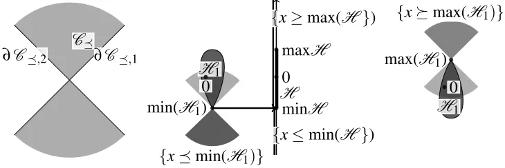
Figure 3 shows the practical appearance of multi-objective maximum/minimum. As

max-imum or minmax-imum must be the tip of the cone moreover, this maxmax-imum/minmax-imum must be

comparable with the whole set hence the whole set must be inside the cone. This gives a drop

shape to the set and strongly delimits range of usability of the multi-objective optimization.

2.3.1. Maximal and minimal optimum. The maximum or minimum solutions to single

objec-tive optimization problems give global solutions - a best choice against any other selection. We

will now investigate the case when a process under the control of a multi-objective optimal

solution drifts out to a state not comparable with the optimal solution in use.

The nature of non-comparable vectors. Let us consider the situation on figure 4 where a turning

vehicle’s movement is analysed. To cover the centripetal force from the static friction of the

r

Kin rF C_{sa f e}

non-comparable

off the road

E>rF

rF safe

E<rF

FIGURE 4. Safe turning formulated with the kinetic energy and the turning radius.

F_{f r}. Using the formula for the needed force to turn at a radius r while having v speed gives us

Fcp=

mv2 r =

2E_kin

r <Ff r. This leads to the safety cone: The turning is safe ifEkin<r F_{f r}

2 =rF (F is a constant defined by the formula). As figure 4 shows, a non-comparable objective vector

leads to disaster. The car movement becomes independent from the intentions of the controller.

He/she has no effect on the movement of a car in such a situation since the brake, the accelerator

and the steering are all based on the friction force which is switched off. Many other examples

show the same situation. Therefore, we may conclude:

Conclusion 1. A selected optimal solution is valid only over the situations with dominated objective vectors. Hence each optimal solution has a domain where it acts. An attempt to use it

outside the domain may lead to a disaster.

Using the conclusion that the optimal solution controls dominated situations only we will

introduce maximal and minimal elements in an object space such that such elements are in the

domain and dominate all comparable elements in the domain.

Definition 6. Let H ⊂Rp and let C be the positive cone of the order relation. Then the

maximal and minimal elements are

max_w,C(H)∈H fulfilsxmaxw,C(H), ∀x∈H comparable with maxw,C(H);

minw,C(H)∈H fulfils minw,C(H)x, ∀x∈H comparable with minw,C(H);

Remark 1. As Figure 5 shows, H ∩ {x max(H )}= /0 which means there is no larger

element inH than the maximal element. Similarly,H ∩{min(H )x}=/0 which means that

0

C

H

max(H )

min(H) max(H )

min(H )

{x≺min(H )}

{xmax(H )}

{x≺min(H )}

{xmax(H)}

FIGURE 5. Multi-objective maximal and minimal solutions.

comparable with the maximal/minimal elements or elements less than or equal to the maximal

element or greater than or equal to the minimal element.

3. OPTIMALFRONTIER.

We essentially concluded in the previous sections that the maximal or minimal optimality

concepts suit more the multi-objective optimization because these concepts require to fulfil the

least conditions equivalent to the guarantee that there is no better option in the object space.

These solutions must be boundary points of the objective space since they themselves must

be in the objective space and any neighbourhood of them must contain points from outside the

objective space (see the reasoning in remark 1). Therefore, the objective space will be assumed

to be a closed set. It also follows from the discussion represented on figure 5 that there are many

minimal or maximal points to a problem.

Any two different optimal solutions may be either comparable or non-comparable. When

comparable, out of two maximal solutions the larger takes care of the smaller one and out of

two minimal solutions the smaller one takes care of the other one.

Definition 7. IfC is a positive cone on the objective space H ⊂Rp then ∀x,y∈H, Cx:=

x+C&C_y:=y+C are comparable ifx∈C_y∨y∈C_xThe relationC_x is comparable toC_yis

denoted byCx∼cCy.

C

M₁ M₂

pvirtual

0

FIGURE 6. Two non-comparable Multi-objective maximums.

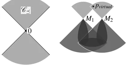
If we form the equivalence classes of all solution cones overH and form the union of cones

in each of the equivalence class, we get a system of optimal cones equivalent to the original

system of optimal solutions which are pairwise non-comparable. Hence comparable pairs of

solutions can be eliminated by selecting one out of any two. Therefore, we may assume that

any two different optimal solutions are non-comparable. Example of non-comparable solutions

is shown on figure 6. Non-comparable maximal or minimal solutions occur when non of the

tips of such cones is in the other cone.

Definition 8. LetH ⊂Rp be the objective space and let C be the positive cone of the order

relation. Then the optimal frontierFopt,max(H):={maxw,C|maxw,C =u∈∂H}. Similarly,

Fopt,min(H):={minw,C|minw,C =u∈∂H}.

The concept originates from Pareto in optimality theory developed in 1910 and was published

in (6). His concept of dominating elements (definition 1) actually shows that his multi-objective

solutions dominate points other than the maximal/minimal solutions. However, Pareto’s order

relation is defined by the cone of positive quadrant (in p-dimensional caseC_Pareto;= n

∏

[0,∞)j

which is a special selection of order relation.

To cover all points of an objective space with dominating cones requires to create optimal

strategy for all the border points in the direction. Such family of solutions is the optimal frontier.

Figure 7 shows the structure of optimal frontier.

Note that having an infinite system of optimal strategies does not make life easy because one

should be used at a time. This leads us to the problem of synthesis which offers an optimal

C

0

FIGURE7. Infinite number of multiobjective solutions.

4. SYNTHESIS OF OPTIMAL SOLUTIONS.

4.1. The switch cone. When a system is controlled by an optimal strategy this strategy has to be changed when the system movement reaches the boundary point of the domain of the optimal

control. If the state point of the system is close to the boundary of the domain of the newly

selected strategy then soon after switching one may expect another switching. Hence knowing

the position of the current state we should select a new optimal strategy where the current state

is relatively far from the boundary of the newly selected optimal behaviour. This requirement

for the selection is solved by introducing a switch-cone as shown on figure 8. Figure 9 shows

the use of switching cones on the optimal frontier.

4.2. Strategy on compact subsets of objective space. Any real system operates in a sub-optimal way and the strategy directs the process towards the sub-optimal operation. There are two

reasons for this: The information as basis of decisions is never complete and the operations

are always subject to random effects. In addition, having infinite set of strategies, at the border

points one has to change strategy for each change of working point which already and

impos-sible requirement from practical point of view. Therefore, we will assume that a system moves

within a compact subset of the object space at a distance from the boundary. This can be covered

by switching cones hence reaching the boundary of the domain of a strategy, there is a switching

cone containing the current state vector hence the system can switch to the new strategy. Figure

0 C

unit lenght H_L,a K_L,a _K˜_,

η

S

FIGURE 8. The definition of the switchcone.

C

0

FIGURE 9. Introduction of switching zones to select more lasting strategies.

∂C,1

∂C,2

C

0

FIGURE 10. Building the objective set from an increasing system of compact

sets, we can cover each set with finite system of switching cones. This gives a

C

0

c

α2=S(x2)

α1=S(x1)

α0=S(x0)

x0 x1

x2

α1

α0

α2

FIGURE11. The constructed synthesis function and its use.

4.3. The synthesis and its use. The interior of a closed set can be obtained as a countable union of ascending sequence of compact sets. If there is a member of such a sequence which

is needed for our operations, then there is a finite subset of the frontier points such that the

corresponding switching cones cover the selected compact set. These cones can be combined

into a finite pairwise disjoint covering of the selected compact set so that reaching the boundary

point of the domain of the currently used optimal strategy, there is a unique strategy to continue

with. The situation is shown on figure 11. This synthesis facilitates stability and asymptotic

analysis of the solution if a dynamical system (ordinary differential equations etc.) model is

created to describe the system’s operation.

5. SOLUTIONMETHODS.

An arsenal of methodologies and techniques has been developed to solve multi objective

optimization problems. We noted earlier in the statement of problem to this presentation that it

is very interesting to generate the local optimal solutions but to successfully give an instructional

guide on how to run a multi-objective system is much more complex than generating these

optimal solutions.

In this lecture we give a comparison among three methods: Scalarization, Pareto’s method

rela-S_c

C∗_pareto

C_∗,pareto

0 0 C

FIGURE 12. The tower shows four ordering cones: The positive coneC, outer

and inserted pareto conesC_paret∗ ,C∗,paret and the scalar coneSc.

tion, Pareto and scalariztion methods.

In line with the multi-objective optimization, the existence of an order relation is defined in

terms of a convex positive coneC. It is known that a convex cone is intersection of hyperplanes

and any finite subsystem of these hyperplanes containsC. If we select n such hyperplanes,

their intersection is a cone spanned by a polygon the sides of this cone gives a pareto basis

(with axes not parallel with the original basis). Look at the cone C∗pareto ⊃C. Also, C

contains a polygon base coneC∗pareto⊂C. Finally all containsScstraight line which is a one

dimensional cone.

We state a lemma to show the relationship among the four cones on Figure 12.

S_c

C∗_pareto

C∗,pareto

P₁ C

S_c

C∗_pareto

C∗,pareto

P₂ C

S_c

C∗_pareto

C∗,pareto

P₃ C

FIGURE 13. The figure shows the relationship between the set of objective

val-ues and the existence of the various maximal points: One may notice that S_c

optimum always exists while the external pareto, the positive cone and the

inter-nal Pareto may not exist.

Sc

C∗_pareto

C∗,pareto

0 0

FIGURE 14. In this case there is no multi-objective optimal solution, not even

forSc.

to C₂;

2. If maxC2(H) is maximal and {maxC2(H)≺ x∈C1}= /0 then maxC2(H) is maximal with respect to C₁. The same holds for minimal elements in the opposite direction.

Corollary 2. In the chain of positive cones a maximal element with respect to any positive cone is maximal with respect to S_c. The same holds for minimal elements.

The corollary states that scalarization gives solution to a maximisation/minimisation

prob-lem, but out of the scalarized solutions one has to select the maximal/minimal ones with respect

to the selected positive cone.

Figure 13 shows that the four positive cones represent different orderings, and on different

objective spaces they give different results. Figure 14 shows that there can be a case such that

there is no optimal solution inside an enclosed loop. Maximal solutions will exist if the tip of

the cone group goes on the top of the boundary points.

Conclusion 2. In this paper we pointed out that the significant differences between single and multi-objective optimizations originate from the existence of a unique complete ordering

com-patible with the vector structure in one dimension against the higher dimensional vector spaces,

infinite inequivalent partial orderings compatible with the vector structure. The existence of

non-comparable vectors in higher dimension lead to limited concept of maximum/minimum and

infinite non-comparable inequivalent optimal solutions to a problem. This leads to the necessity

of synthesis techniques for the creation of a practical control guide for the user.

Remark:

This paper is a summary of some of the results from the Ph.D. thesis (15) of Obikwere, Clare

A. supervised by Dr. Effanga, E. O. and Prof. Z. Lipcsey.

Conflict of Interests

The authors declare that there is no conflict of interests.

REFERENCES

[1] O. AUGUSTO, F. BENNIS, ANDS. CARO,A new method for decision making in

multiob-jective optimization problems, Pesquisa Operacional, 32 (2012), pp. 331–369.

[2] G. B. DANTZIG ANDB. C. EAVES,Fourier–motzkin elimination and it dual, Journal of

Combinatorial Theory, (A) (1973), pp. 288–297.

[3] K. DEB, Multi-objective Optimization using Evolutionary Algorithms, New York: Wiley,

[4] E. V. DENARDO,Linear Programming and Generalizations- A Problem-based

Introduc-tion with Spreadsheets, vol. 149, Springer Verlag, 2011.

[5] F. Y. EDGEWORTH, Mathemtical Physics: An Essay on the Application of Mathematics

to the Moral Sciences, C. Kegan and Paul and Co., 1881.

[6] M. EHRGOTT,Vilfredo pareto and multi-objective optimization, Documenta Mathematica,

(2010), pp. 447–453.

[7] G. GORDON AND R. TIBSHIRANI, Karush–kuhn–tucker conditions, Optimization,

(2014), pp. 10–36.

[8] W. J. GUTJAHR AND A. PICHLER,Stochastic multi-objective optimization: a survey on

non-scalarizing methods, Annals of Operations Research, Special volume (2013).

Au-thors: Department of Statistics and Operations Research University of Vienna, Austria

and Norwegian University of Science and Technology, Norway.

[9] C. L. HWANG AND A. S. MASUD, Multiple Objectives Decision Making?Methods and

Applications, Springer, 1979.

[10] J. JAHN,Vector Optimization, Springer Verlag, 2011.

[11] T. C. KOOPMANS,Analysis of production as an efficient combination of activities, 1951.

[12] H. W. KUHN ANDA. W. TUCKER,Nonlinear programming, in Second Berkeley

Sympo-sium Proceedings on mathematical Statistics and Probability, J. Ney-man, ed., University

of California Press, Berkeley, 1951, pp. 481–492. Princeton University and Stanford

Uni-versity.

[13] R. T. MARLER AND J. S. ARORA, Survey of multi–objective optimization methods for

engineering, Struct Multidisc Optim, 26 (2004), pp. 369–395.

[14] C. J. NASH, The (dantzig) simplex method for linear programming, in The (Dantzig)

Simplex Method for Linear Programming, no. 1521–9615/00/10.00 A9 2000 IEEE in The

Top Ten Algorithms, University of Ottawa, 2000.

[15] C. A. OBIKWERE, Tools and Alternative Solution Techniques for Multi-objective

Opti-mization, PhD thesis, University of Calabar, 2016.

[16] V. PARETO,Manuale di Economia Politica, Societa Editrice Libraria, Milano, Italy, 1906.

York. 1971.

[17] P. PARRILO AND S. LALL, Fourier-motzkin elimination, Stanford University, (2003),

pp. 1–29.

[18] V. TKINDT ANDJ. BILLAUT,Multicriteria Scheduling: Theory, Models and Application,

Springer-verlag, 2006.