Tire demand planning based on reliability and operating environment

International Journal of Mining and Geo-Engineering

* Corresponding author. Tel.: +98-9149405561.

E-mail address: [email protected] (A. Nouri Gharahasanlou).

DOI: 10.22059/ijmge.2016.59875

Journal Homepage: ijmge.ut.ac.ir

Tire demand planning based on reliability and operating environment

A. Nouri Gharahasanlou

a*

_{, M. Ataei}

a

_{, R. Khalokakaie}

a

_{, B. Ghodrati}

b

_{, R. Jafarie}

c

a _{Faculty of Mining, Petroleum & Geophysics, Shahrood University of Technology, Shahrood, Iran}

b _{Luleå University of Technology, Luleå, Sweden}

c Sahand University of Technology, Iran

ARTICLE HISTORY

Received 02 Aug 2016, Received in revised form 07 Dec 2016, Accepted 11 Dec 2016

ABSTRACT

Tires are of critical spare parts in mines. There is a shortage of medium and large tires. In addition, since the mining activities and opening new mines has increased, the demand for tires has increased significantly as well. Thus, it is very important for mining engineers to identify the tire characteristics and properly manage the spare part inventory. Spare parts management is critical from an operational perspective, especially in intensive industries assets, such as mining, as well as in organizations that own and operate costly assets. A knowledge of the tires’ behavior (historical data) must be taken into account along with the operating environment conditions (covariates). This study uses Cox multiple regression model to incorporate machine operating environment information into systems reliability analysis for estimation of spare parts. It considers a proportional hazard model and a stratified Cox regression model for time independent and dependent covariates. Based on the results, the study develops a mathematical model for spare parts estimation at the component level for non-repairable parts (tires). It validates the outcomes using a case study of loader tires in the Sungun mine in Iran. There is a significant difference in the results of spare parts forecasting and inventory management when considering and dismissing the covariates.

Keywords: Operating environment; Proportional hazard model; Reliability; Spare part; Stratified cox regression model

1. Introduction

However, it is not possible to design a system without failures. Poor reliability and maintainability characteristics, combined with poor maintenance and inadequate product support strategy, often lead to unscheduled operation suspensions. For most of highly mechanized companies, maintenance costs account for a significant part of the operating budget (reaching 15–70% of production costs), but logistics and spare parts provisioning (SPP) are often considered less essential in strategic thinking. Maintenance of the type of machinery that was described above is expensive not only because of high repair costs, but also more importantly because of the cost of lost products [1–3]. SPP strategy is dependent upon component characteristics such as reliability and the environment in which the system/product is used [1, 4, 5]. Reliability-Based Spare Parts Provision (RSPP), a derivation of SPP, is an effective way to incorporate reliability and operating conditions into the design process.

In 2003, Kumar proposed a service delivery strategy for industrial products with a special reference to mining systems. He studied some of

the factors influencing the service delivery strategy and suggested several approaches to reduce these gaps, thereby satisfying customers and meeting operational demands [2]. A year later, Kumar studied spares and service management from maintenance, repair and operations points of view [6]. Markeset and Kumar addressed approaches to the development of product support strategy to enhance the performance of industrial products. They argued that the product support could be considered as a source of income for the manufacturer in the conventional product paradigm, and as a cost and an obligation in the delivery of performance paradigm [7]. For their part, Chen et al. proposed a multi-echelon spare parts model involving suppliers, distribution centers and equipment users. The model considers both the age-based preventive replacement policy and priority demand classes [8]. Finally, Ghodrati produced comprehensive studies in the spare parts area, including the differences between the Weibull model and exponential model in SPP, the risk of ignoring covariates in spare parts planning, and SPP for the following: brake systems, the lifting cylinder (jack) of loaders, the hydraulic seal of jacks, brake pads (brake lining kit) of a mining loader and an electricity meter in the power distribution system in Jajarm of Iran [1, 3, 4, 9–13].

tires on loaders in the mining industry. The loader tire database used in this study was created over 11 years at Sungun copper mine in Iran. Data gathering is more complicated when it has to be combined with a database of operating environment factors, but spare parts consumption can only reliably be predicted if the covariates of the system, such as the operating environment, are considered along with its reliability characteristics. The absence of coherent algorithm for spare part provision based on the reliability and operating environment complicated the issue as well.

In this paper, the RSPP was used for spare parts estimation. The first step is to identify the reliability performance and the failure rate of the tires based on the operating environment. The next step is to derive the reliability function and consider the independent and time-dependent covariates using the proportional hazard model (PHM) and the stratification approach. Then, based on the reliability performance of the component, the required number of spare parts can be estimated. In this case, the SPP considering tire performance and any influencing factors on the reliability performance (i.e., covariates) was successfully done. Discounting covariates such as the operating environment may lead to erroneous results in reliability performance analysis, and consequently in SPP. Therefore, the main objectives of the paper are to define the coherent algorithms for RSPP, conduct a comprehensive study of the reliability, spare part estimation of the tire component of a loader system and propose an analytical goodness of fit test for the proportionality assumption as an extension of the statistical process.

This paper is organized into three main parts. Part one introduces the theoretical background and definitions of RSPP. In part two, the findings are validated using a case study in the Iranian mining industry. Part three provides the conclusion.

2. The proposed methodology

This section presents the suggested methodology for estimation of spare parts by modeling the effect of covariates on the reliability of a component. Components are defined as the level at which the failure rate data need to be collected or estimated considering the effect of influencing factors. The basic methodology is illustrated in Figure 1. The methodology comprises four main steps:

1. Boundary definitions, assumptions, identification and formulation of covariates, and data collection (time data and covariate data).

2. Explanation of covariate analysis approach and identification of the degree of influence of each covariate on the hazard function (estimation of regression coefficients).

3. Identification of baseline/baselines reliability function/functions and distribution of failure data considering the covariate effects. Spare parts estimation and inventory management.

2.1.Boundaries, assumptions, identification of covariates and data collection

The first step of the methodology is to set boundaries at different levels, such as component, subsystem, and system. A system boundary defines internal components of a system in order to prevent overlaps with adjoining systems. The component boundary clearly defines all boundaries of a specific component with other components in the system through which it interfaces via hardware or software. The exact definitions of component and system restrictions are necessary to apply the equipment reliability parameters in the analysis. It must be noted that only events occurring inside the component boundaries are accounted for analysis [14]. The following basic assumptions and boundaries govern this paper:

 Systems (loaders) consist of s-independent components (tires).

 Only non-repairable components / parts in repairable systems are studied, in other words, one system with special attention to one component.

 Each component and the larger system is in one of two possible states: operating or failed.

 The failure properties of the component are considered.  Maintenance leads to as good as new condition.

 Only the operation and maintenance phases are considered. Research is restricted to a mining working environment (Sungun copper mine).

Data collection is an essential element of reliability analysis. Basic data in reliability analysis for a non-repairable component are the time to failure (TTF) data. Of these fundamental data, all factors influencing the reliability of the component (such as temperature, dust, humanity, etc.), as well as its failure mode and mechanism must be considered during data collection. In addition, the influencing factors must be identified and formulated as covariates. The relevant covariates can have different origins, including the operating environment (e.g. temperature, pressure, humidity, or dust), operating history of a machine (e.g. overhauls, effects of repairs, or type of maintenance), or the type of design or material [4]. Based on the effect of the covariates on reliability, they can be divided into two main groups:

 Categorical covariates: these are qualitative variables. They can be binary or have multiple categories. A binary covariate can be handled in the model by the use of a dummy variable, coded as zero or one. For example, Ghodrati and Kumar assigned the hydraulic oil quality in the brake system −1 for non-standard and non-manufacturer/supplier-recommended brake oil and +1 for standard and manufacturer recommended hydraulic brake oil [4].

 Continuous covariates: these have a defined scale, and can be quantified. They can change linearly or nonlinearly. For example, to study the influence of operating temperature in a mine crushing site, Barabadi and et al. considered average temperature on the day of the maintenance as a covariate value [16].

A frequently occurring problem in the analysis of datasets has been that the data were not collected under the same conditions. Covariates are used to address this problem [17]. The boundary selection also has a direct effect on data collection. The boundary definition has to be compatible with the generated data. Data on reliability characteristics can be obtained directly from the field or sample testing in laboratories [18].

2.2.Covariate analysis

Figure 1. Methodology for provisioning required spare parts considering covariates [4, 14, 15].

2.2.1.Proportional-hazard model (PHM)

The proportional hazard model is a nonparametric regression model that uses a semi-parametric method. The model incorporates a parametric model of the relationship between the failure rate and the

specified covariates. It was used in the present research to calculate the component failure rates [14, 16]. PHM was initially applied in medical analysis before being used in engineering reliability analysis. In general, The PHM is influenced not only by time but also by the covariates under which it operates. This model represents a distribution-free approach to the set of tools used in reliability analysis. It assumes that the hazard rate Define boundary

Establish assumption

Identify and formulate covariates (Influence factors)

Data collection in chronologically ordered (TBFs and codified values of covariates)

Is the proportional hazards (PH) assumption

satisfy? Use basic proportional

hazard model (PHM) regression model (SCRM)Use stratified Cox

Defined parameter of model or regression

coefficient of corresponding n covariates Defined parameter of model or regression coefficient of corresponding n unstratified covariates

Trend? _{Power law process (PLP)}

Identical distributed data

Dependency? Branching Poisson process

or other similar models

Weibull distribution

Spare parts provision

Inventory management requirements Yes

Yes

Yes

No No

No

Defined baseline function or functions for each stratum

1

2

3

of a system/component is a product of an arbitrary and unspecified baseline hazard rate, 𝜆0(𝑡), dependent on time only, and a positive functional term (linear form 1 + 𝛼𝑧 , the log‐linear exp⁡(𝑧𝛼) and a logistic form log⁡(1 + exp⁡(𝛼𝑧) ), basically independent of time, incorporating the effect of a number of explanatory variables or covariates. The common form of the PHM is log‐linear, expressed as Eq.(1) [4, 11]:

𝜆(𝑡. 𝑧) = 𝜆0(𝑡)𝜓(𝑧𝛼) = 𝜆0(𝑡)𝑒𝑥𝑝 (∑ 𝑧𝑖𝛼𝑖 𝑛

𝑖=1

) (1)

The reliability influenced by the covariates is given as [1]:

𝑅(𝑡. 𝑧) = (𝑅0(𝑡))

𝑒𝑥𝑝(∑𝑛𝑖=1𝑧𝑖𝛼𝑖) ₍₂₎

where⁡𝜆(𝑡. 𝑧) and 𝑅(𝑡. 𝑧) are the hazard and reliability functions, respectively; 𝑧𝛼 = ∑𝑛𝑖=1𝑧𝑖𝛼𝑖 ; 𝛼 (column vector) is the unknown parameter of the model or regression coefficient of the corresponding n covariates (z) (row vector consisting of the covariate parameters) indicating the degree of influence of each covariate on the hazard function; and 𝜆0(𝑡) and 𝑅0(𝑡) are the baseline failure rate and baseline reliability, respectively. As mentioned earlier, in the PHM, the proportional assumption (PH assumption) is that the covariates are time-independent variables, so the ratio of each two hazard rates is constant versus time [16]. Various approaches are used to determine whether the (PH) assumption fits a given data set. The graphical procedure, a goodness-of-fit testing procedure, and a procedure involving the use of time-dependent variables are used most widely in PH assumption evaluations [19].

2.2.2. Stratified Cox regression method (SCRM)

The PH assumption may be violated in some cases. In such cases, the stratified Cox regression model (SCRM) can be used to build the model. The stratified Cox model is an extension of the PHM that allows controlling a predictor by “stratification” that does not satisfy the PH assumption. In this model, when there are n levels for the time-dependent covariates, each level is defined as a stratum. Under this circumstance, historical data will be grouped in different strata. Separate baseline hazard rates are computed for each stratum, and the regression coefficients are equal for all strata. The hazard rate in the 𝑠𝑡ℎ _{stratum is} written as [4, 16]:

𝜆𝑠(𝑡. 𝑧) = 𝜆0𝑠(𝑡)𝑒𝑥𝑝 (∑ 𝑧𝑖𝛼𝑖 𝑛

𝑖=1

) ⁡⁡⁡⁡⁡⁡𝑠 = 1.2. … . 𝑟 (3)

As with the original SCRM, there are two unknown components in the model: the regression parameter 𝛼 and the baseline failure function

𝜆0𝑠(𝑡) for each stratum. The baseline failure functions for r remain completely unrelated in the different strata.

2.3.Identification of baseline/baselines reliability function/functions The baseline hazard rate is assumed to be equal to the total hazard rate when the covariates have no influence on the failure pattern. The shape of the baseline repair rate and the regression coefficients for the covariates may be estimated by using the historical data or by using the input from experts [16]. Here, the baseline hazard rate is modeled using parametric models and stochastic processes. Two main stochastic processes are generally used for reliability analysis: renewal process (RP) and nonhomogeneous Poisson process (NHPP).

As shown in Figure 1, in order to determine the best analytical method for available data, the trend and serial correlation tests must be performed to determine whether the data are independent and identically distributed (iid). The trend test can be done analytically or graphically [15, 20, 21]. There are three analytical methods for testing the presence of trends: Military Handbook test, Laplace test, and Anderson-Darling. If the null hypothesis for the P-value of these tests is rejected at the 5% level of significance, it means that the TBF data show

a trend and, therefore, are not identically distributed. In graphical methods, the trend test involves plotting the scaled cumulative failure numbers against the scaled cumulative time to failure. If the plotted points lie (or approximately lie) on a straight horizontal line, the data are trend-free [22]. For the results of the trend test, if the assumption that the data are identically distributed is rejected, a non-stationary model must be fitted, such as the power low process (PLP).. The power law process (PLP), a form of the nonhomogeneous Poisson process (NHPP), has proved to be a useful tool for analyzing the systems that are deteriorating or improving through time passage. The PLP model was found to be very suitable for modeling the reliability of systems [23]. A graphical test for serial correlation can also be done by plotting the ith TBF against the (i-1)th TBF, i = 1; 2; ...; n. If the plotted points are randomly scattered without any pattern, there is no correlation among the TBFs, and the data are independent. The presence of no trend and no serial correlation in the data means that the data are iid, and the two-parameter Weibull distribution, a classical statistical technique, is the best choice for baseline hazard rate modeling [15, 20, 21]. The Weibull distribution is widely used for reliability data, particularly the data on strengths of materials and failure times [24]. The two-parameter Weibull distribution can represent decreasing (shape parameter < 1), constant (shape parameter = 1), or increasing failure rates (shape parameter >1). These correspond to the three periods of the "bathtub curve" of engineering system reliability, also called "burn-in," "useful life," and "wear-out" phases of life [25].

2.4.Spare parts estimation

Production and manufacturing companies are under great pressure to decrease their production costs to stay cost effective. Industrial operation cost analysis shows that, in general, maintenance comprises a significant proportion of the overall operating cost. Spare parts availability is a major issue in the maintenance process; increased availability of spare parts leads to increased availability of equipment and minimized total production costs [3]. “Spare parts” refer to the parts needed to keep equipment in a healthy operating condition by meeting repair and replacement needs caused by failures or preventive and corrective maintenance. Spare parts management, as a form of product support, can be defined as a trade-off between managing inventory and meeting service levels. This translates into a need for accuracy and high analytical capabilities [6]. Identifying the right type of inventory management system for a manufacturing firm can be a difficult and complex task. As spare parts for machinery are regularly of a very high quality, the problem cannot be solved simply by increasing the warehouse stock [3].

RSPP is a popular mathematical model used in spare parts provisioning based on renewal theory. The renewal process can be used whenever the failure rate is not constant. If the failure rate is constant, the homogeneous Poisson process is used as a special case of a renewal process to forecast demands for spares. It is important to note that the above statement is valid only for non-repairable spares (components) [4]. In this case, the renewal theory was used to analyze the replacement of the component upon failure (the time to failure or time between replacements), to find the distribution of the number of replacements, and to determine the mean number of replacements. In short, the reliability measure of a component is used to estimate the required number of spares [3].

If the operation time (and planning horizon) t of the machine in which the part (component) is installed is too long and several replacements must be made during this period, the average number of failures in time t, E[N(t)] = M(t), will stabilize to the asymptotic value of the function as [3, 18]:

𝑀(𝑡) = 𝐸[𝑁(𝑡)] =𝑡 𝑇̅+

𝜁2_{− 1}

2 (4)

𝜁 =𝜎(𝑇)

𝑇̅ (5)

where 𝑇̅ is the average time to failure for replacements of a part, and

𝜎(𝑇) is the standard deviation of the time to failure [3, 18].

If the time of planning horizon (t) is large, then N(t) in Eq.(4) has approximately a normal distribution (based on a central limit theorem) with mean = 𝑁(𝑡)̅̅̅̅̅̅. The approximate number of spares (𝑁𝑡) needed during the period of a planning horizon with a probability of shortage =

1 − 𝑝 is given by [3, 18]:

𝑁𝑡= 𝑡 𝑇̅+

𝜁2_{− 1}

2 + 𝜁√

𝑡 𝑇̅Φ

−1_{(𝑝) (6)}

where Φ−1_{(𝑝) is the inverse normal distribution function.}

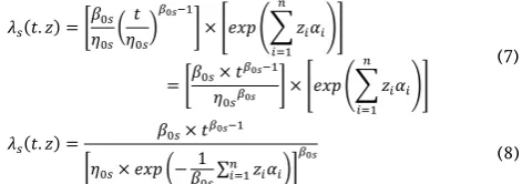
As shown in Figure 1, the two-parameter Weibull reliability model and power low process (PLP) are versatile models for characterizing the case of iid (no trend and no serial correlation) and trend-bearing data of mechanical parts, respectively. The appearance and format of the hazard occurrence of the PLP model is the equivalent of the two-parameter Weibull distribution [4, 23, 26]. Thus, integrating the effect of covariates into the PHM and SCRM can be respectively defined by the following equations [3, 18]:

𝜆𝑠(𝑡. 𝑧) = [ 𝛽0𝑠 𝜂0𝑠

( 𝑡 𝜂0𝑠

) 𝛽0𝑠−1

] × [𝑒𝑥𝑝 (∑ 𝑧𝑖𝛼𝑖 𝑛

𝑖=1 )]

= [𝛽0𝑠× 𝑡 𝛽0𝑠−1

𝜂0𝑠𝛽0𝑠

] × [𝑒𝑥𝑝 (∑ 𝑧𝑖𝛼𝑖 𝑛

𝑖=1 )]

(7)

𝜆𝑠(𝑡. 𝑧) =

𝛽0𝑠× 𝑡𝛽0𝑠−1

[𝜂0𝑠× 𝑒𝑥𝑝 (−_𝛽1 0𝑠∑ 𝑧𝑖𝛼𝑖

𝑛 𝑖=1 )]

𝛽0𝑠 (8)

where 𝛽0𝑠 and 𝜂0𝑠 are the initial (baseline) shape and scale parameters, respectively, for each stratum in SCRM ("s" subscript suffix is limited for PHM). This equation indicates the Weibull distribution or PLP with the shape parameter (𝛽𝑠) and scale parameter (𝜂𝑠), written as [3, 4, 18]:

{

𝛽𝑠= 𝛽0𝑠

𝜂𝑠= 𝜂0𝑠[𝑒𝑥𝑝 (∑ 𝑧𝑖𝛼𝑖 𝑛

𝑖=1 )]

−_𝛽1

0𝑠 (9)

Therefore, the influencing covariates in the Weibull distribution and the PLP change the scale parameter, while the shape parameter remains unchanged [3].

The 𝑇̅𝑠 and 𝜎𝑠(𝑇) of the Weibull distribution and the PLP can be calculated based on the shape and scale parameter, expressed as [3, 4, 18]:

𝑇̅𝑠= 𝜂𝑠Γ (1 + 1 𝛽𝑠

) (10)

𝜎𝑠(𝑇) = 𝜂𝑠√Γ (1 + 2 𝛽𝑠

) − Γ2_{(1 +}1 𝛽𝑠

) (11)

2.5.Spare parts inventory management

Inventory control of spare parts is playing an increasingly crucial role in modern operations management. The exchange is clear: on one hand, a large number of spare parts conditions the capital, while on the other hand, too little inventory may result in poor customer service or extremely costly emergency actions [18].

The economic order quantity (EOQ) can be used to reach a balance. EOQ refers to the size through which the total inventory cost is minimized; it considers aspects of holding and ordering with a perspective of eliminating shortages and can be calculated as [18].

𝐸𝑂𝑄 = √2𝐷𝑆

𝐻 (12)

where "D" is the annual demand (units/year)[equals 𝑁𝑡 in one year], "S" is the cost of ordering or setting up one lot ($/lot), and "H" is the cost of holding one unit in the inventory for a year (often calculated as a proportion of the item’s value).

To use a “continuous review system” in inventory control and management, the “reorder point (ReP)” need to be calculated that expressed as [1]

𝑅𝑒𝑃 = 𝑑 × 𝐿 + 𝜎̅̅̅̅̅̅̅̅̅̅̅̅̅̅̅̅̅̅𝐷× √𝐿Φ_{(𝑝 2}⁄ ) (13)

where d is the average demand, L is the lead time, Φ

(𝑝 2⁄ ) is the confidence level of cycle service, and 𝜎𝐷 is the number of standard deviations from the mean, calculated as [1]

𝜎𝐷= √ 𝑡

𝑇̅. (14)

3. Case study

All industries rely on productivity to generate profits. If the vital productivity equipment fails, the production is lost. In mining industries, the loader machine is pivotal to production; the loader loads the ore or waste rocks from the mining fronts into the trucks. When a loader breaks, the profit is lost. Loss of profit does not stop the mining loader alone. A maintenance crew must be summoned to inspect and solve the problem. A disabled loader may also delay or block other machines in the extraction cycle. Thus, maintaining a fleet of haul trucks and loading equipment is crucial for maintaining the productivity.

An investigation of a fleet of loaders at Sungun copper mine in Iran shows that the rock moving systems are critical subsystems, and the tire is the most important part of this subsystem.

Sungun copper deposit is the second largest copper mine in Iran. The geological reserve of the deposit is estimated to have a reserve of up to 828 million tons, with an average copper grade of 0.62%. During the time of investigation, the mine operation was managed by a fleet of 12-wheel loaders belonging to a contracting company.

3.1.Data collection and covariate formulation

Appropriate data collection is one of the most important steps in reliability analysis. A data collection system must be designed to facilitate correct and effective reliability analysis. The data in this research were obtained from the field observations. Although it is an expensive and time-consuming procedure, field data are the most representative part of a tire reliability and maintainability characteristics [18]. The failure data were not collected for reliability study purposes. The company had compiled the operation data, maintenance cards, inventory lists, tire department data, and meteorological data sheets for a fleet of loader machines over 11 years, from 2003 to 2014. It was not easy to sort the required information, so searching the data lasted two years. For preliminary investigation of the statistical nature of the data, the critical component of these machines and the influencing covariates, and several interviews were held with machine operators, maintenance crews, and management.

value indicates the tires censored failure, and a cell with the value unity indicates tire failure. The last column of the table shows the total time to failure.

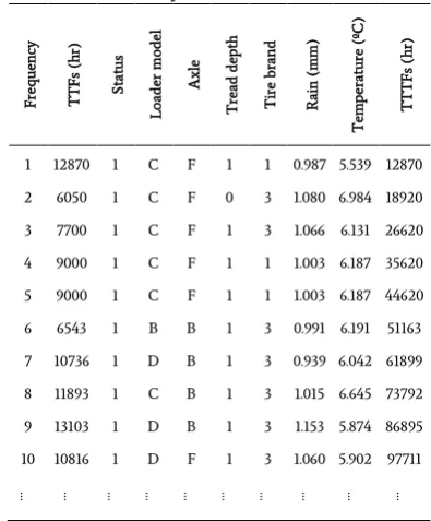
Table 1. Sample TTF data for loader tire.

Fre

que

nc

y

T

T

Fs

(h

r)

Sta

tus

Lo

ad

er

m

od

el

A

xl

e

T

re

ad

d

ep

th

T

ir

e

bra

nd

R

ain

(m

m

)

T

em

pe

ra

tur

e

(º

C

)

T

T

T

Fs

(

hr)

1 12870 1 C F 1 1 0.987 5.539 12870

2 6050 1 C F 0 3 1.080 6.984 18920

3 7700 1 C F 1 3 1.066 6.131 26620

4 9000 1 C F 1 1 1.003 6.187 35620

5 9000 1 C F 1 1 1.003 6.187 44620

6 6543 1 B B 1 3 0.991 6.191 51163

7 10736 1 D B 1 3 0.939 6.042 61899

8 11893 1 C B 1 3 1.015 6.645 73792

9 13103 1 D B 1 3 1.153 5.874 86895

10 10816 1 D F 1 3 1.060 5.902 97711

… … … …

To formulate the tire covariates, we used observation, repair shop cards and reports, and the experience of managers, operators, and maintenance crews, along with field data. The covariates are shown in Table 1 and include the following items:

 Loader model (z11,z12and z ): Three different model loaders 13

are used by the contracting company. A tire in Sungun mine could work on one specific model of loader in its whole lifetime or can be changed between two models. Table 2 shows the codified covariate; three dummy variables,

z

₁₁

,

z

₁₂and

z

₁₃, are assigned to

formulate it.

Table 2. Codified loader model covariate.

Model Code

z

11

z

12

z

13

Komatsu wheel loader WA470-3 A 1 0 0

Komatsu wheel loader WA600-3 B 0 1 0

Caterpillar wheel loader 988B C 0 0 1

Komatsu WA600-3 & Caterpillar 988B D 0 0 0  Axle (

z

₂): The tires are installed in the front (F) and the back (B)

axle of the loader. A dummy variable,

z

₂, is assigned to denote

the axle position. Table 3 shows the codified covariate by a dummy variable.

Table 3 - Codified loader axle covariate Axle Code z2

Back B 1

Front A 0

 Tread depth (

3

z

): The tread depth has a direct effect on the

lifetime of the tire. The tread depth is denoted by covariate

z

₃, and its value is divided by two, the depth of each tire tread (to avoid a small regression factor for covariates). The covariates are assigned the value 1 for a depth less than or equal to 10 mm and zero for a depth greater than 10 mm.

 Tire Brand (

z

₄): Three main tire brands are used in Sungun

mine. The covariate

z

₄ is assigned to show the brand type; 1 represents Bridgestone, 2 represents Triangle or Goodyear and 3 represents all other brands.

 Climatic conditions, including rain (

z

₅) and temperature (

z

₆): Temperature in the mine site ranges from -2.69 ºC in the winter to +16.37 ºC in the summer. Rain ranges from 0.26 mm to 1.97 mm. During the winter or on a rainy day, maintenance crews wear thick gloves, warm jackets, and rain jackets. The covariates

z

₅and

6

z

are assigned to the rain and temperature, respectively. The average temperature and average rain in the month of the maintenance activity are used for the covariate values.

3.2.Reliability analysis of tires

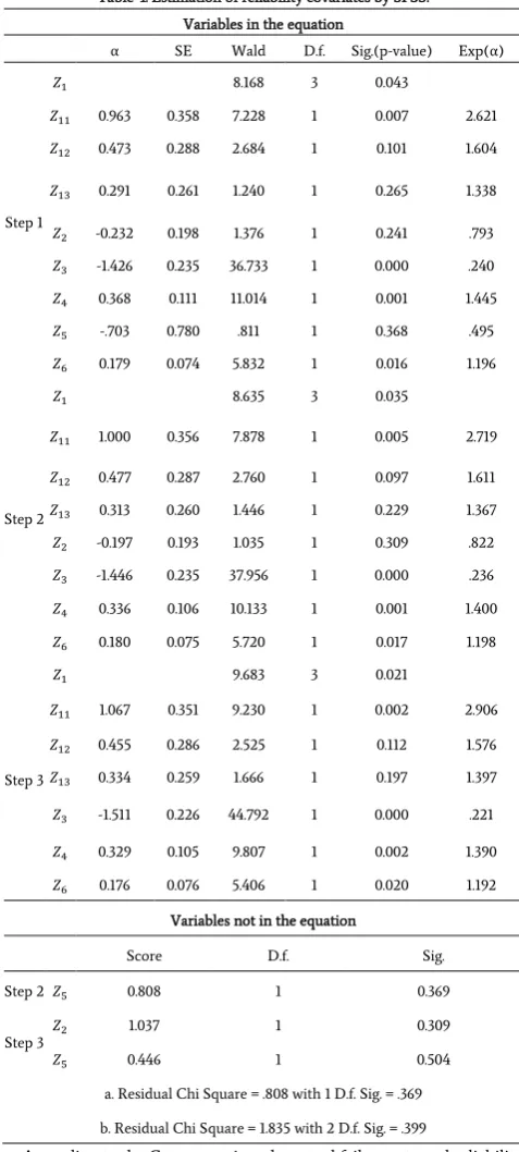
In Cox regression analysis, when there is a little theoretical reason to prefer one model type to another, stepwise methods of covariate selection can be useful. The estimation of the effect of a covariate in the Cox model may be biased if significant influential covariates are not considered; therefore, the covariates with no significant value are eliminated in subsequent calculations.

Several methods are available for selecting independent variables; stepwise methods (forward and backward) is a common approach. Stepwise methods can use the Wald statistic, the likelihood ratio, or a conditional algorithm. In stepwise methods, the score statistic is used to select variables for the model. In this study, corresponding estimates of

α are obtained by a backward stepwise method and tested for their significance based on the Wald statistic (P-value). IBM SPSS Statistics software, version 22, was used to estimate the value of the regression vector. The asymptotic distribution of the Wald statistic is chi-square with degrees of freedom equal to the number of parameters estimated. The stepwise variable selection process using the backward stepwise procedure (BSTEP) can be defined as follows [27]:

1. Estimate the parameters for the full model, using the final model from the previous procedure and all eligible variables. Only variables listed on the BSTEP variable list are eligible for entry and removal. Let the current model be the full model. 2. Based on the MLEs of the current model, calculate the Wald

statistic for every variable in the model and find its significance. 3. Choose the variable with the largest significance. If that significance is less than the probability required for variable removal (significant at the 10% level), go to step 5. Otherwise, if the current model without the variable with the largest significance is the same as the previous model, stop BSTEP; if not go to step 4.

4. Modify the current model by removing the variable with the largest significance. Estimate the parameters for the modified model and return to step 2.

5. Check to see if any eligible variable is not in the model. If all are included, stop BSTEP; otherwise, go to the next step.

6. Based on the MLEs of the current model, calculate the score statistic for every variable not in the model and find its significance.

7. Choose the variable with the smallest significance. If that significance is less than the probability of variable entry, go to the next step; otherwise, stop BSTEP.

8. Add the variable with the smallest significance to the current model. If the model is not the same as any of the previous models, estimate the parameters for the new model and return to step 2; otherwise, stop BSTEP.

are represented using dummy coding; that is, the dummy corresponding to the reference category simply was omitted. Also note that the stepwise method includes parameters for dummy variables, but excludes the intercept in the analysis. The significance of dummy variable 𝑍1 is 0.021, i.e., less than the probability of variable entry; therefore, its intercept (𝑍11. 𝑍12.𝑍13) is excluded from analysis.

Table 4. Estimation of reliability covariates by SPSS. Variables in the equation

α SE Wald D.f. Sig.(p-value) Exp(α)

Step 1

𝑍1 8.168 3 0.043

𝑍11 0.963 0.358 7.228 1 0.007 2.621

𝑍₁₂ 0.473 0.288 2.684 1 0.101 1.604

𝑍₁₃ 0.291 0.261 1.240 1 0.265 1.338

𝑍2 -0.232 0.198 1.376 1 0.241 .793

𝑍₃ -1.426 0.235 36.733 1 0.000 .240

𝑍4 0.368 0.111 11.014 1 0.001 1.445

𝑍₅ -.703 0.780 .811 1 0.368 .495

𝑍6 0.179 0.074 5.832 1 0.016 1.196

Step 2

𝑍₁ 8.635 3 0.035

𝑍11 1.000 0.356 7.878 1 0.005 2.719

𝑍₁₂ 0.477 0.287 2.760 1 0.097 1.611

𝑍13 0.313 0.260 1.446 1 0.229 1.367

𝑍₂ -0.197 0.193 1.035 1 0.309 .822

𝑍3 -1.446 0.235 37.956 1 0.000 .236

𝑍4 0.336 0.106 10.133 1 0.001 1.400

𝑍6 0.180 0.075 5.720 1 0.017 1.198

Step 3

𝑍₁ 9.683 3 0.021

𝑍11 1.067 0.351 9.230 1 0.002 2.906

𝑍12 0.455 0.286 2.525 1 0.112 1.576

𝑍₁₃ 0.334 0.259 1.666 1 0.197 1.397

𝑍3 -1.511 0.226 44.792 1 0.000 .221

𝑍4 0.329 0.105 9.807 1 0.002 1.390

𝑍6 0.176 0.076 5.406 1 0.020 1.192

Variables not in the equation

Score D.f. Sig.

Step 2 𝑍5 0.808 1 0.369

Step 3 𝑍2 1.037 1 0.309

𝑍5 0.446 1 0.504

a. Residual Chi Square = .808 with 1 D.f. Sig. = .369

b. Residual Chi Square = 1.835 with 2 D.f. Sig. = .399

According to the Cox regression, the actual failure rate and reliability function of the tire component considering the environment can be presented respectively as:

𝜆(𝑡. 𝑧) = 𝜆0(𝑡)𝑒𝑥𝑝(𝑧1𝛼1+ 𝑧3𝛼3+ 𝑧4𝛼4+ 𝑧6𝛼6) (15)

𝑅(𝑡, 𝑧) = (𝑅0(𝑡))

𝑒𝑥𝑝(𝑧1𝛼1+𝑧3𝛼3+𝑧4𝛼4+𝑧6𝛼6)

(16)

The hazard ratio should be constant throughout the passage of time; that is, the proportionality of hazards from one covariate to another should not vary over time. This assumption is known as the proportional hazards assumption (PH assumption). Graphical approaches are commonly used to assess the PH assumption by comparing log–log survival curves. Parallel curves, say comparing two different values of a covariate, indicate that the PH assumption is satisfied. The graphical approach has some problems, however. The main problem is “how parallel is parallel?” This decision can be very subjective for a given dataset, particularly if the study size is relatively small. Another problem is how to categorize a continuous variable, like temperature. If many categories are chosen, the data “thin out” in each category, making it difficult to compare different curves. A final problem is how to evaluate the PH assumption for several variables simultaneously. Goodness-of-fit (GOF) tests represent an alternative way to assess the PH assumption.

This study draws on the test of Harrel and Lee (1986), a variation of a test originally proposed by Schoenfeld (1982) and based on the residuals defined by Schoenfeld, now called the Schoenfeld residuals. The GOF testing approach is appealing because it provides a test statistic and p-value (P(PH)) for assessing the PH assumption for a given predictor of interest. Thus, the researcher can make a more objective decision using a statistical test than is typically possible in a graphical approach. P(PH) is used to evaluate the PH assumption for the variable of interest. An insignificant (i.e., large) P(PH), say, greater than 0.10, suggests that the PH assumption is reasonable, whereas a small P(PH), say, less than 0.05, suggests that the variable being tested does not satisfy this assumption [28]. Table 5 gives the mean values and the statistical GOF test outcomes for the tire data.

Table 5. Statistical test approach results for PH assumption.

Covariates Means Coeff. (Pearson Correlation) P(PH)

𝑍11 0.116 0.066 0.442

𝑍12 0.268 -0.158 0.065

𝑍13 0.464 0.061 0.447

𝑍₃ 0.616 0.034 0.689

𝑍4 1.652 -0.144 0.092

𝑍6 6.676 0.044 0.606

Correlation is significant at the 0.01 level

The P(PH) values given in this table provide GOF tests for each variable in the fitted model adjusted for the other variables in the model. The P(PH) values are quite high for all variables satisfying the PH assumption. Thus, according to Figure 1, the PHM can be used to assess the covariates of the tires. With the results obtained from SPSS in Table 5, the actual failure rate and operational reliability considering the environmental conditions can be presented respectively as:

𝜆(𝑡. 𝑧) = 𝜆0(𝑡)𝑒𝑥𝑝(1.067𝑧11+ 0.455𝑧12+ 0.334𝑧13

− 1.511𝑧3+ 0.329𝑧4+ 0.176𝑧6) (17)

𝑅(𝑡. 𝑧) = (𝑅0(𝑡))

𝑒𝑥𝑝(1.067𝑧11+0.455𝑧12+0.334𝑧13−1.511𝑧3+0.329𝑧4+0.176𝑧6) (18)

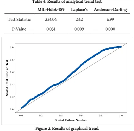
The results of the analytical and graphical trend tests carried out on the TTF tire data using Minitab software are shown in Table 6 and Figure 2. The null hypothesis (H0: No trend) is violated at a 5%

Table 6. Results of analytical trend test.

MIL-Hdbk-189 Laplace’s Anderson-Darling

Test Statistic 226.04 2.62 6.99

P-Value 0.031 0.009 0.000

Figure 2. Results of graphical trend.

A test for serial correlation is done by plotting the ith TTF against the (i-1)th TTF, i = 1; 2; 3;…; n. The results indicate no correlation in general among the TTFs. Therefore, the assumption that the data are iid is not valid, and the NHPP method is the best choice for baseline hazard function modeling and analysis. This research selected the PLP, a special form of the NHPP, to analyze the baseline hazard function of the tire. Because of the polynomial nature of the rate of occurrence of a failure, this model is very flexible and can model both increasing and decreasing baseline hazard rates.

Next, the parameters of the baseline PLP model are estimated analytically using ReliaSoft's RGA software. According to the calculations, 𝛽0=1.221 and 𝜂0=15900. Based on these parameters, the operational failure rate and operational reliability considering the environmental conditions are represented respectively as:

𝜆(𝑡. 𝑧) = [1.221 15900(

𝑡 15900)

0.221 ]

× [𝑒𝑥𝑝(1.067𝑧11+ 0.455𝑧12+ 0.334𝑧13− 1.511𝑧3 + 0.329𝑧4+ 0.176𝑧6)]

(19)

(20)

𝑅(𝑡. 𝑧)

= (𝑒𝑥𝑝 (− 𝑡 15900)

1.221 )

𝑒𝑥𝑝(1.067𝑧11+0.455𝑧12+0.334𝑧13−1.511𝑧3+0.329𝑧4+0.176𝑧6) (21)

(22) In these equations, Exp(α) is the hazard ratio. This ratio indicates the expected changes in the risk of a terminal event when the covariate’s categories change, or for continuous covariates, the ratio predicts change in the hazard rate for each unit increase in the covariate. If Exp(α) is less than 1.0, the direction of the effect is a reduction in the hazard rate. If the value 1.0 appears within the confidence intervals of a covariate, the effect of that covariate is considered insignificant. The result of the analysis shows that 𝑧2 and 𝑧5 play less important roles than the other factors, such as 𝑧3 and 𝑧5, on tire reliability. It may also be concluded that the failure rate of the loader system in a Komatsu WA470-3 wheel loader is exp(1.067) times greater than that of the other models. The effect of covariates 𝑧12, 𝑧13 and 𝑧3 can be explained similarly. However, 𝑧11 plays a more important role than the other covariates on the reliability performance of the tires.

The results of the covariate analysis can assist managers and performance engineers. Based on the results, they may decide that the

𝑧1, 𝑧3, 𝑧4 and 𝑧6 factors need to be controlled or improved to avoid component failures. In the manufacturer perspective, some of these parameters can be considered during the design stage of a system or component.

The reliability and hazard rate of the tire for the Komatsu WA470-3

loader and other models is now calculated and plotted for the mean value of other covariates, as shown in Figure 3. The results show the tires on the Komatsu WA470-3 loader are less reliable than the tires on other loaders. As can be seen, their reliability reaches about 42% after about 2000 hr of operation and zero after about 7000 hr of operation. There is a 70% and a 75% chance that tires will work without failure for 1000 hr in a Komatsu WA470-3 loader and the other models, respectively. The results can obviously help engineers and managers to make decisions about operation planning, maintenance strategy, sales contract negotiations, spare parts management etc.

Figure 3. Comparison of reliability performance of tires in Komatsu WA470-3 loader and other models.

Totally, operational conditions have significant effects on reliability performance and should be considered carefully in both design and operation phases. Otherwise, the system’s targets reliability performance may not be reached.

3.3.Required spare parts estimation for loader

When a machine fails, the operator (inspector or sensors) reports the failure and the failed part has to be sent to the field depot workshop. If the field depot has the spare part on hand and a technician is available, the technician travels to the site to fix the machine. Otherwise, the repair is delayed until a technician is available to fix the machine or the spare part becomes available at the field depot. In either case, the delay is very costly to the customer. The workshop of Sungun mine is always active, so a technician is available at any time. In this case, it is necessary to correctly manage spare parts to achieve high-quality service and shorten the response time.

On one hand, spare parts are expensive and sometimes have high depreciation and obsolescence costs, for instance, electronic components. Therefore, it is imperative to keep the inventory level as low as possible at the central warehouse and the field depots. On the other hand, mining managers are often faced with a shortage of required spare parts when making decisions based on the manufacturer’s/supplier’s recommendations. In most cases, the manufacturer is unaware of the prevailing environmental factors when estimating the average number of required spare parts. Yet the actual reliability of a system is a function of the length of operation and the environment under which it operates. To calculate the spare parts for different operating conditions in the case study mine, 12 scenarios for the two most efficient covariates (loader model and tire brand) were defined as shown in Table 7.

Using Eqs. (6), (10), (11), and (17) the required number of spare parts for each scenario can be calculated for the next three years in a short-term production plan. According to the mine production plan, annual operating time is 7668 hours.

1.0 0.8 0.6 0.4 0.2 0.0 1.0

0.8

0.6

0.4

0.2

0.0

Scaled Failure Number

S

ca

le

d

T

o

ta

l

T

im

e

o

n

T

e

st

0.0000 0.0001 0.0002 0.0003 0.0004 0.0005 0.0006 0.0007 0.0008

0 0.1 0.2 0.3 0.4 0.5 0.6 0.7 0.8 0.9 1

0 1000 2000 3000 4000 5000 6000 7000

H

az

ard

ra

te

R

el

ia

bil

ity

(%

)

Time (Hr)

R (Z11=Komatsu WA470-3) R (Z11=Other Model)

Table 7. Scenarios over three years in Sungun mine.

Sc

en

ari

o

Lo

ad

er

m

od

el

T

re

ad

d

ep

th

Description

Covariates

𝒁𝟏𝟏 𝒁𝟏𝟐 𝒁𝟏𝟑 𝒁𝟑∗ 𝒁𝟒 𝒁𝟔∗

1 A 1 Komatsu - WA470-3 with

Bridgestone tire 1 0 0 0.616 1 6.676

2 A 2 Komatsu - WA470-3 with

Triangle or Goodyear tire 1 0 0 0.616 2 6.676

3 A 3 Komatsu - WA470-3 with the

other tire brands 1 0 0 0.616 3 6.676

4 B 1 Komatsu - WA600-3 with

Bridgestone tire 0 1 0 0.616 1 6.676

5 B 2 Komatsu - WA600-3 with

Triangle or Goodyear tire 0 1 0 0.616 2 6.676

6 B 3 Komatsu - WA600-3 with the

other tire brands 0 1 0 0.616 3 6.676

7 C 1 Caterpillar - 988B with

Bridgestone tire 0 0 1 0.616 1 6.676

8 C 2 Caterpillar - 988B with

Triangle or Goodyear tire 0 0 1 0.616 2 6.676

9 C 3 Caterpillar - 988B with the

other tire brands 0 0 1 0.616 3 6.676

10 D 1

Komatsu WA600-3 & Caterpillar 988B with Bridgestone tire

0 0 0 0.616 1 6.676

11 D 2

Komatsu WA600-3 & Caterpillar 988B with Triangle

or Goodyear tire

0 0 0 0.616 2 6.676

12 D 3

Komatsu WA600-3 & Caterpillar 988B the other tire

brands

0 0 0 0.616 3 6.676

∗: 𝑍3 and 𝑍6= mean value of covariates

Using Eqs. (6), (10), (11), and (17) the required number of spare parts for each scenario can be calculated for the next three years in a short-term production plan. According to the mine production plan, annual operating time is 7668 hours.

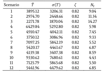
Note that when the covariates are ignored (𝑒𝑥𝑝(∑𝑛𝑖=1𝑧𝑖𝛼𝑖) = 0), the required number of tires is 3.07. This estimation is not accurate enough, because in real situations, as discussed earlier, several covariates influence the reliability characteristics of tires. Table 8 shows the required number of spare parts for the different scenarios with 5% probability of shortage. The calculation shows that the value of 𝑁𝑡 in all scenarios is greater than 3.07. This difference is considerable in spare parts forecasting and inventory management.

Table 8. Required number of spare parts for different scenarios over three years.

Scenario 𝑇̅ 𝜎(𝑇) 𝜁 𝑁_𝑡

1 3895.12 3206.31 0.82 9.04 2 2974.70 2448.66 0.82 11.34 3 2271.78 1870.04 0.82 14.27 4 6429.84 5292.80 0.82 5.98 5 4910.47 4042.11 0.82 7.45 6 3750.12 3086.96 0.82 9.33 7 7097.25 5842.19 0.82 5.52 8 5420.17 4461.67 0.82 6.87 9 4139.38 3407.38 0.82 8.59 10 9330.62 7680.61 0.82 4.43 11 7125.79 5865.68 0.82 5.50 12 5441.96 4479.62 0.82 6.85

As shown in Figure 3 and Table 8, lower reliabilities mean a greater probability of an unexpected number of failures, leading to unscheduled repairs and a consequent increase in the required number of spare parts. The spare parts calculations for scenario 1 compared to scenarios 4, 7 and 10, for scenario 2 compared to scenarios 5, 8 and 11, and for scenario 3 compared to scenarios 6, 9 and 12 allverify this hypothesis.

As Table 8 shows, the Caterpillar - 988B loader is the best choice from the spare parts cost point of view (scenarios 7, 8, 9) and the Komatsu - WA470-3 loader is the most costly model (scenarios 1, 2, 3). However, there is no big difference between the required tires for the Komatsu - WA600-3 and the Caterpillar -988B loaders (scenarios 10, 11, 12). In other words, both can be used. In addition, all loader models using Bridgestone tires require fewer spare parts than the loaders using other brands. Thus, the life cycle of Bridgestone tire is longer than the life cycle of the other tires, as seen in the 𝑇̅ column. Triangle, Goodyear and the other brands follow the order.

3.4.Loader tires inventory management requirements The following assumptions were considered:

 The cost of one tire equals 10,000 USD$  The cost of ordering one lot equals 145 USD$

 The annual holding cost equals 1000 USD$ of the part cost  The average lead-time is 10 days

 Cycle service confidence level is 90%

The economic order quantity (EQO) and reorder point (ReP) with respect to annual demand rates in different scenarios are calculated based on Eq. (12) and (13) and tabulated in Table 9.

Table 9. Economic order quantity.

Scenario 1 2 3 4 5 6 7 8 9 10 11 12

EOQ 1.04 1.15 1.29 0.85 0.95 1.05 0.82 0.91 1.01 0.74 0.82 0.91

ReP 0.99 1.14 1.31 0.77 0.88 1.01 0.73 0.84 0.96 0.63 0.73 0.84

Whenever the inventory position reaches 0.99 units/loader tire, we should order 1.04 units/loader tire for scenario 1. However, where no covariate exists, the EOQ and RP of tires are equal to 0.62 and 0.5 respectively. In comparison, the EOQ and RP in both conditions, with or without considering the operating environment's effect, illustrate the significance of these factors and their role in the actual life of the parts. In other words, the operating environment parameters should be considered in the process management of machines, in this case, the loaders.

4. Conclusions

Since the tire prices are increasing and the increased downtime decreases the performance reliability, the optimization of tire management is very important. Tires are crucial spare parts with a significant impact on both productivity and costs of mine production. Mining engineers must have an understanding of how tires work, how tires fail, and how to optimize the tires life for mining projects to be as profitable as possible. The operating condition of tires and the performance index, such as reliability, are the two important elements that mining engineering could use for effective management of tires. This study considers reliability and the operating environment to estimate spare parts for loader tires in Sungun mine in Iran. Forecasting the spare parts based on the reliability characteristics of an item is one of the most effective strategies for preventing unplanned stoppages due to lack of spare parts. For effective forecasting, all factors that influence the reliability characteristics of the item need to be treated as covariates in the reliability analysis.

have a significant effect on the reliability characteristics of the loader tire and, consequently, on the required number of spare parts. The noticeable difference in spare parts estimation caused by including (case 1) and dismissing (case 2) the covariates for different scenarios verifies this. The calculation of the economic order quantity and reorder point shows around 50% difference between the two cases.

REFERENCES

[1] Ghodrati B., Kumar U., Kumar D. (2003). Product support logistics based on product design characteristics and operating environment. Society of Logistics Engineers, Huntsville, United States, p 21

[2] Kumar U. (2003). Service delivery strategy for mining systems. Application of Computers and Operations Research in the Minerals Industries South African Institute of Mining and Metallurgy 43–48.

[3] Ghodrati B., Banjevic D., Jardine A. (2010). Developing effective spare parts estimations results in improved system availability. IEEE, pp 1–6

[4] Ghodrati B., Kumar U. (2005). Reliability and operating environment-based spare parts estimation approach: a case study in Kiruna Mine, Sweden. Journal of Quality in Maintenance Engineering 11,169–184.

[5] Barabadi A. (2012). Reliability and Spare Parts Provision Considering Operational Environment: A Case Study. International Journal of Performability Engineering 8, 497. [6] Kumar S. (2004). Spare Parts Management–An IT Automation

Perspective. Domain Competency Group, Infosys Technology Limited

[7] Markeset T., Kumar U. (2005) Product support strategy: conventional versus functional products. Journal of Quality in Maintenance Engineering 11, 53–67.

[8] Chen M-C., Hsu C-M., Chen S-W. (2006). Optimizing joint maintenance and stock provisioning policy for a multi-echelon spare part logistics network. Journal of the Chinese Institute of Industrial Engineers 23, 289–302.

[9] Ghodrati B. (2006). Weibull and Exponential Renewal Models in Spare Parts Estimation: A Comparison. International Journal of Performability Engineering 2, 135.

[10] Ghodrati B., Kumar U. (2005). Operating environment-based spare parts forecasting and logistics: a case study. International Journal of Logistics Research and Applications 8, 95–105. doi: 10.1080/13675560512331338189

[11] Ghodrati B., Akersten P-A., Kumar U. (2007). Spare parts estimation and risk assessment conducted at Choghart Iron Ore Mine: A case study. Journal of Quality in Maintenance Engineering 13, 353–363.

[12] Ghodrati B., Benjevic D., Jardine A. (2012). Product support

improvement by considering system operating environment: A case study on spare parts procurement. International Journal of Quality & Reliability Management 29, 436–450. doi: 10.1108/02656711211224875

[13 Barabadi A., Ghodrati B., Barabady J., Markeset T. (2012). Reliability and spare parts estimation taking into consideration the operational environment a case study. IEEE, pp 1924–1929 [14] Barabadi A., Barabady J., Markeset T. (2011). A methodology for

throughput capacity analysis of a production facility considering environment condition. Reliability Engineering & System Safety 96, 1637–1646.

[15] Barabady J., Kumar U. (2008). Reliability analysis of mining equipment: A case study of a crushing plant at Jajarm Bauxite Mine in Iran. Reliability Engineering & System Safety 93, 647– 653. doi: 10.1016/j.ress.2007.10.006

[16] Barabadi A., Barabady J., Markeset T. (2011). Maintainability analysis considering time-dependent and time-independent covariates. Reliability Engineering & System Safety 96, 210–217. [17] Kumar D., Klefsjö B. (1994). Proportional hazards model: a

review. Reliability Engineering & System Safety 44, 177–188. [18] Ghodrati B. (2005). Reliability and operating environment based

spare parts planning. Luleå University of Technology [19] Kleinbaum DG. (2011). Survival analysis. Springer

[20] Hoseinie SH., Ataei M, Khalokakaie R., Kumar U. (2011). Reliability modeling of water system of longwall shearer machine. Archives of mining sciences 56, 291–302.

[21] Hoseinie SH., Ataei M., Khalokakaie R., Kumar U. (2011). Reliability modeling of hydraulic system of drum shearer machine. Journal of Coal Science and Engineering (China) 17, 450–456. doi: 10.1007/s12404-011-0419-3

[22] (210AD) Minitab® 16.2.0, Help.

[23] Hoseinie H., Ataei M., Khalokakaie R., et al (2012). Reliability analysis of the cable system of drum shearer using the power law process model. International Journal of Mining, Reclamation and Environment 1–15. doi: 10.1080/17480930.2011.622477 [24] Smith RL. (1991). Weibull regression models for reliability data.

Reliability Engineering & System Safety 34, 55–76.

[25] Dhillon BS. (2008). Mining equipment reliability, maintainability, and safety. Springer

[26] Kumar D., Klefsjö B., Kumar U. (1992). Reliability analysis of power transmission cables of electric mine loaders using the proportional hazards model. Reliability Engineering & System Safety 37, 217–222. doi: 10.1016/0951-8320(92)90126-6

[27] IBM - United States. http://www.ibm.com/us-en/. Accessed 10 Nov 2015