https://doi.org/10.5194/gmd-12-735-2019 © Author(s) 2019. This work is distributed under the Creative Commons Attribution 4.0 License.
Similarities within a multi-model ensemble:
functional data analysis framework
Eva Holtanová1, Thomas Mendlik2, Jan Koláˇcek3, Ivanka Horová3, and Jiˇrí Mikšovský1
1Department of Atmospheric Physics, Faculty of Mathematics and Physics, Charles University, V Holešoviˇckách 2, Prague, 180 00, Czech Republic
2Wegener Center for Climate and Global Change, University of Graz, Brandhofgasse 5/1, Graz, 8010, Austria 3Department of Mathematics and Statistics, Faculty of Science, Masaryk University, Kotláˇrská 267/2, 611 37, Brno, Czech Republic
Correspondence:Eva Holtanová ([email protected]) Received: 25 June 2018 – Discussion started: 14 August 2018
Revised: 3 December 2018 – Accepted: 28 January 2019 – Published: 19 February 2019
Abstract.Despite the abundance of available global climate model (GCM) and regional climate model (RCM) outputs, their use for evaluation of past and future climate change is often complicated by substantial differences between in-dividual simulations and the resulting uncertainties. In this study, we present a methodological framework for the anal-ysis of multi-model ensembles based on a functional data analysis approach. A set of two metrics that generalize the concept of similarity based on the behavior of entire simu-lated climatic time series, encompassing both past and future periods, is introduced. To our knowledge, our method is the first to quantitatively assess similarities between model sim-ulations based on the temporal evolution of simulated values. To evaluate mutual distances of the time series, we used two semimetrics based on Euclidean distances between the simu-lated trajectories and based on differences in their first deriva-tives. Further, we introduce an innovative way of visualizing climate model similarities based on a network spatialization algorithm. Using the layout graphs, the data are ordered on a two-dimensional plane which enables an unambiguous in-terpretation of the results. The method is demonstrated using two illustrative cases of air temperature over the British Isles (BI) and precipitation in central Europe, simulated by an en-semble of EURO-CORDEX RCMs and their driving GCMs over the 1971–2098 period. In addition to the sample results, interpretational aspects of the applied methodology and its possible extensions are also discussed.
1 Introduction
While numerical climate models serve as the cardinal tool of contemporary climatology, their outputs are typically bur-dened by distinct uncertainties, manifesting through substan-tial differences between individual simulations. Here, we ad-dress the issue of comparing various climate simulations and quantifying their differences by introducing a methodology for analysis of multi-model ensembles and the relationship between nested regional climate model simulation and its driving global climate model (GCM) run. We propose use of a metric generalizing the concept of similarity, based on the information contained in the entire simulated climate series, extending from historical to future periods. The evaluation framework is based on functional data analysis (further de-noted as FDA; Ramsay and Silverman, 2005, 2007; Ferraty and Vieu, 2006).
ary conditions. Estimating the uncertainty range based on the MME spread is not a straightforward task, as currently available MMEs suffer from various deficiencies. One obsta-cle is raised by the deficiencies in the statistical experimental design: models are developed voluntarily from institutions worldwide. This problem is further amplified when designing an ensemble of RCMs. An RCM is driven by a GCM, which has a substantial effect on the nested simulation (Déqué et al., 2007, 2012; Heinrich et al., 2014). It is not computation-ally feasible to run all combinations of RCMs with every GCM. Therefore, for a proper uncertainty assessment it is crucial to investigate the interactions between driving GCMs and nested RCMs and their respective influence on the total MME spread (e.g., Déqué et al., 2012; Holtanová et al., 2014; Heinrich et al., 2014; Holtanová and Mikšovský, 2016).
In addition, climate models (even across developing in-stitutions) are known to share certain components, leading to inter-model similarities and dependencies. This makes it difficult to justify the independence assumption when quan-tifying the uncertainty of MMEs with standard statistical models. Recently, innovative methods have been developed to identify groups of similar climate models (e.g., Knutti et al., 2013) and account for the similarities (Annan and Harg-reaves, 2017). However, these methods quantify model sim-ilarity based on either their behavior in approximating the historical climate or purely on their projected climate change signals. Some studies included evaluation of the relationship between the driving GCM and nested RCM based on more advanced climatic characteristics (e.g., Rajczak and Schär, 2017; Crhová and Holtanová, 2018), but their approach to the issue was rather qualitative. To our knowledge, our method is the first to quantitatively assess similarities between model simulations based on the temporal evolution of simulated val-ues.
To illustrate a possible application of the proposed methodology we analyze similarities and dissimilarities be-tween members of the EURO-CORDEX multi-model en-semble (Jacob et al., 2013) and their driving GCMs. The inter-model distances between the trajectories of the tempo-ral development of running 30-year mean changes in sea-sonal mean air temperature and precipitation are evaluated.
FDA approach. Section 4 explains the application of method-ological framework, and Sect. 5 is devoted to description of the results of the case study. Section 6 summarizes key fea-tures of the proposed framework and offers possible further applications.
2 Data
The methodological framework is presented with the sam-ple of RCM simulations from the EURO-CORDEX initia-tive (Jacob et al., 2013; http://www.euro-cordex.net/, last ac-cess: 30 April 2018) together with their driving GCMs. We use 13 RCM simulations driven by nine different GCMs. All RCM simulations have 0.44◦horizontal resolution. The RCM simulations were conducted for the period 1951–2100, with some of them starting in 1971 or ending in 2098. We therefore concentrate on the period 1971–2098. After the year 2006 model simulations incorporated the representative concentration pathway RCP8.5 (van Vuuren et al., 2011). The GCM simulations were performed under the CMIP5 protocol (Taylor et al., 2012). The list of models is given in Table 1, and the GCM–RCM simulation matrix is given in Table 2. To identify individual simulations, we use the acronyms consisting of the abbreviations for the RCM and GCM (as defined in Table 1) connected with the underscore character. In the case of the driving GCM simulation, we use “dGCM” instead of the RCM identification.
Table 1.List of regional climate models and driving global climate models incorporated in the present study. The first column contains the acronyms used throughout the text. The type column indicates whether the model is regional (RCM) or global (GCM).
Acronym Type Model ID Institute
CCLM RCM CCLM4-8-17 Climate Limited-area Modelling Community (CLM-Community)
REMO RCM REMO2009 Helmholtz-Zentrum Geesthacht, Climate Service Center, Max Planck Institute for Meteorology
RCA4 RCM RCA4 Swedish Meteorological and Hydrological Institute – Rossby Centre
ALAD RCM ALADIN53 Centre National de Recherches Météorologiques
CUNI RCM RegCM4 Charles University
CanESM GCM CanESM2 Canadian Centre for Climate Modelling and Analy-sis
CNRMCM GCM CNRM-CM5 Centre National de Recherches Météorologiques – Météo-France; Centre Europeén de Recherches et de Formation Avancée en Calcul Scientifique
CSIROx GCM CSIRO-Mk3.6.0 CSIRO; Queensland Climate Change Centre of Ex-cellence
GFDLES GCM GFDL-ESM2M NOAA Geophysical Fluid Dynamics Laboratory
HadGEM GCM HadGEM2-ES Met Office Hadley Centre
IPSLCM GCM IPSL-CM5A-MR Institut Pierre Simon Laplace, Paris, France
MIROC5 GCM MIROC5 University of Tokyo, National Institute for Envi-ronmental Studies, Japan Agency for Marine-Earth Science and Technology
MPIESM GCM MPI-ESM-LR Max Planck Institute for Meteorology
NorESM GCM NorESM1-ME Norwegian Climate Centre
Table 2.Matrix of regional climate model simulations and their driving global climate models that are incorporated in the present study.
Driving global climate models
CanESM CNRMCM CSIROx GFDLES HadGEM IPSLCM MIROC5 MPIESM NorESM
Re
gional
climate
models
CCLM x
RCA4 x x x x x x x x x
ALAD x
CUNI x
REMO x
3 Methodology
3.1 Functional data analysis approach
We analyzed similarities and dissimilarities between the tem-poral development of simulated 30-year running mean air
temperature and precipitation changes. The original dataset consisted of simulated valuesyik at central years of the
30-year periods, tk,k=1, ..., K, ranging from 1986 to 2083
(henceK=98) for each model,i=1, ...,n. These sequences of simulations were converted to functional form using the
Figure 1. (a)Temporal development of running 30-year mean changes in winter (DJF) mean air temperature (changes of running 30-year mean averages throughout the period 1971–2098 in comparison to the reference period 1971–2000) averaged over the British Isles region. (b)Smoothed functional data from(a), created as described in Sect. 3. The lines in both panels are colored according to the driving global climate model (GCM), and the type of line corresponds to regional climate model (RCM). The acronyms of the model simulations are explained in Sect. 2; dGCM stands for the driving global climate model simulation.
Figure 2.The same as Fig. 1, but for running year mean changes in summer (JJA) mean precipitation (relative changes of running 30-year mean averages throughout the period 1971–2098 in comparison to the reference period 1971–2000), averaged over the eastern European region.
was approximated by a spline functionxi(t )in the form
xi(t )= XN
j=1cijBj(t ), i=1, . . ., n. (1) TheB-splinesBj(t )were polynomials of order four with 20
equally spaced knots, and cij values were real coefficients
in theB-spline basis. Such use of order-four B-splines im-plied N=22 basis functions. Spline functions xi(t ) were
constructed in order to minimize the penalized squared er-ror
Xn
i=1
XK
k=1
yij−xi(tk) 2
+λ
tK Z
t1
d2
dt2xi(t )
2
dt, (2)
with respect to the coefficientscij. The smoothing parameter
λ was selected via the validation method. The
cross-validation method was based on the minimization of the fol-lowing expression:
Xn
i=1
XK
k=1
yij−xi(tk, λ,−k)
2
, (3)
where xi(tkλ,−k) denotes the leave-one-out estimator of
xi(t )omitting thek-th observation (tk, yik). The actual
cal-culation is based on minimization of the error ofxi(t, λ,−k)
using a smoothing operator – see, for example, Craven and Wahba (1978) for details. The representative examples of the functional data from panel (a) of Figs. 1 and 2 are depicted in panel (b) of the respective figures.
sameB-spline basis with coefficientscij0 :
xi0(t )=XN
j=1c 0
ijBj(t ), i=1, . . ., n. (4)
All subsequent analyses were conducted separately for both
xi(t )andxi0(t ).
For the representation of functional data in statistical soft-ware R (R Core Team, 2013), we used the package fda (Ram-say et al., 2017). It provides several basis options for func-tional data including theB-splines presented above and fur-ther functional data processing techniques.
Since the time series analyzed in the present study are rel-atively smooth, a metric and a semimetric were constructed to represent the distance separation between two curves (note that the smaller the cross distance, the more similar the two curves are). Such an approach seems to be appropriate, e.g., Pokora et al.(2017). Let f1 and f2 be two curves, specifi-cally two cubic smoothing splines in our case. A well-known and widely-used distance between given curvesf1andf2is theL2metric,d0(f1, f2). It is a nonnegative number, whose square is defined as the integral
d02(f1f2)=
tK Z
t1
f1(t )−f2(t ) 2
dt. (5)
Let us call this common metricd0distance (Euclidean dis-tance).
Similarly, a common way to build a semimetric between two curves is to consider the L2 distance between the first derivatives of the curves. More precisely, given two curvesf1 andf2, we define thed1distanced1(f1, f2)as a nonnegative number, whose square is given by the integral
d12(f1f2)=
tK Z
t1
f10(t )−f20(t )2dt. (6)
Figure 3 illustrates examples of two parts of time series that are evaluated as quite different with a large distance
d0=112.8 but are similar with a relatively small distance
d1=1.56. The main point is that the values of the semimet-rics are inferred solely based on the chosen feature (e.g., Eu-clidean distance for d0) and are independent of other time series characteristics. In Fig. 3 it is clearly seen that unlike
d0, thed1semimetric does not take into account the mutual bias of the two time series. It only focuses on the character of their temporal development. The analysis of sensitivity to the amount of smoothing was carried out. The mutual distances of the curves do not strongly depend on the smoothing pa-rameter, as shown in Figs. 4 and 5.
3.2 Visualization of the similarities
For visualization of mutual distances based on FDA semi-metrics we use layout graphs created using the ForceAt-las2 algorithm (Jacomy et al., 2014) within the Gephi soft-ware (https://gephi.org/, last access: 31 May 2018). In these
Figure 3.Illustration of the functional data analysis approach for evaluation of time series similarity. The two arbitrarily chosen time series shown here (Model 1 and 2) are evaluated to be quite different when based ond0but are similar when based ond1.
graphs individual members of the multi-model ensemble are visualized as nodes (each model simulation corresponding to a single node). The ForceAtlas2 algorithm creates a force-directed layout of the underlying data. The network of the nodes is created by simulating a physical system and its movement. The nodes are repulsed from each other in anal-ogy to charged particles. At the same time the edges between the nodes attract them like springs (Jacomy et al., 2014). The iterative procedure of finding the nodes positions results in an equilibrium state which corresponds to the final network. The interpretation of the layout graphs is straightforward. The closer the nodes are to each other, the lower the mu-tual distance of corresponding simulations, according to the semimetric of interest. The larger the node, the higher the number of close neighbors, meaning more similar simula-tions (with similarity defined by the values of selected semi-metric). The edges between nearest 10 % of neighbors are made visible. The colors indicate the driving GCM.
4 Application of the methodology
Figure 4.Normalizedd0distances between simulated air temperature curves (data are shown in Fig. 1a) of randomly selected model and other models, which depend on amount of smoothing. Starting values representd0distances between original curves, and values at the end representd0distances for oversmoothed data. The vertical line depicts the amount of smoothing used in the presented study.
Figure 5.The same as Fig. 4, but for distancesd1.
pixel plot (see Figs. 6 and 7) with a temperature–color code (or heat map, with a redder color for more similarity and a brighter color for less similarity).
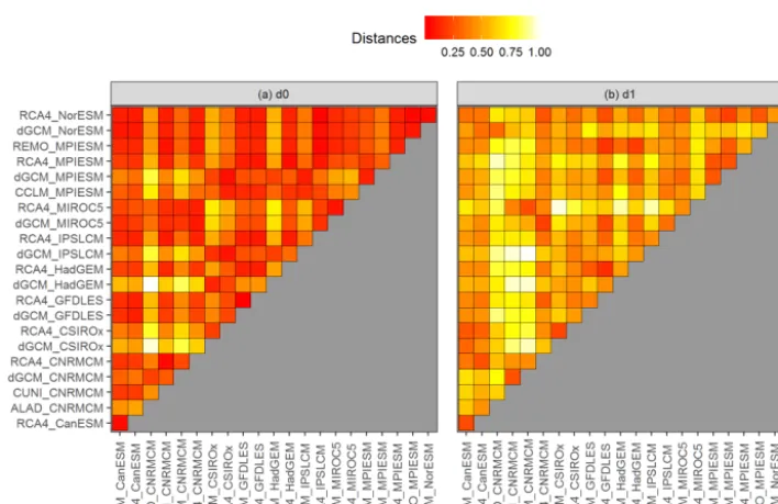
Figures 6 and 7 present the values of d0 (panel a) and
d1(panel b) distances for the two chosen datasets presented in Figs. 1 and 2. Firstly, there are clear differences be-tween the evaluation based on d0 andd1 semimetrics, be-cause each of them is based on different aspects of evalu-ated curves. It is well apparent from the comparison of max-imum distances. In the case of JJA pr over EA (Fig. 7), the d0 distance is the largest for the driving HadGEM GCM (dGCM_HadGEM) and ALADIN RCM driven by CN-RMCM (ALAD_CNCN-RMCM). These two simulations effec-tively represent lower and upper bounds of the multi-model
ensemble (Fig. 2). In contrast, according tod1the most dis-similar time series are GCM simulations by IPSLCM and CNRMCM (Fig. 7b), because their temporal development has largely an opposite sign, even though they do lie “inside” the multi-model ensemble (Fig. 2).
inter-Figure 6. (a)Heat map of thed0distances for running 30-year mean changes in winter (DJF) mean air temperature over British Isles (the curves are shown in Fig. 1b, underlying data are shown in Fig. 1a) with redder color for more similarity and brighter color for less similarity between respective curves. The values of the semimetricd0are scaled to the interval [0,1]. The acronyms of the model simulations are explained in Sect. 2. The definition of the distances is explained in Sect. 3.1.(b)is the same as(a), but ford1distances.
Figure 7.The same as Fig. 6, but for running 30-year mean relative changes in summer (JJA) mean precipitation over eastern European region (the curves are shown in Fig. 2b, underlying data are shown in Fig. 2a).
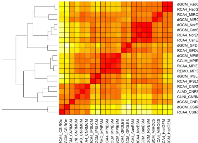
pretation of the dendrograms might not be straightforward, and relatively similar simulations might be assigned to quite remote clusters. In our example (Fig. 8) this is the case for the simulations of HadGEM and CNRM GCMs which are assigned to two remote clusters, even though their mutual
similar-Figure 8.An example of the dendrogram resulting from hierarchical cluster analysis based ond1distances for running 30-year mean changes in winter (DJF) mean air temperature over British Isles (underlying similarity matrix in Fig. 6b).
ities based on evaluated semimetrics distances, using the lay-out graphs (see Sect. 3.2). Figures 9 and 10 show the laylay-out graphs for the two investigated cases. The main advantage of the layout graphs in comparison to classical dendrograms is that the structure of the ensemble is shown in 2-D, therefore the mutual distances are seen easily. The relationships noted above between the HadGEM, MIROC5 and CNRM clusters are easily interpreted using the layout graph (Fig. 9b).
5 Case study results
The methodology described in Sect. 3 was applied to the modeled temperature and precipitation changes from the EURO-CORDEX multi-model ensemble and the respective driving GCMs for eight large European domains (Chris-tensen and Chris(Chris-tensen, 2007). Here we only show two cases in order to illustrate the ability of the proposed method to as-sess the relationships within the members of the multi-model ensemble. These two sample cases, DJF tas over BI and JJA pr over EA, were chosen because they differ in terms of the results obtained by application of the proposed methodology, and the results are quite illustrative.
Since we analyze simulations incorporating RCP8.5, which assumes a rise in greenhouse gas concentrations dur-ing the whole 21st century, it is not surprisdur-ing that all models give a rise in DJF near surface air temperature over the BI region throughout this period (Fig. 1). The RCMs tend to give a generally lower temperature change than their driving GCMs, except for RCMs driven by CNRMCM, MPIESM
and MIROC5. Regarding the simulated changes in summer mean precipitation over the EA region (Fig. 2), the model simulations disagree on the sign of precipitation change, and the multi-model ensemble has quite a large variance. Some RCMs project larger changes than their driving GCMs (e.g., ALADIN driven by CNRMCM), and some give smaller changes (RCA4 driven by IPSLCM).
Based ond0, the distances calculated for JJA pr over EA are mostly quite low (lower than 0.25) with a couple of out-liers, namely ALAD_CNRMCM and driving simulations of HadGEM and CSIRO (Fig. 7a). Thed0distances for DJF tas over BI are more evenly distributed (Fig. 6a), because there are not so many distinct outliers. Thed1distances are higher thand0values in both regions and are generally higher for JJA pr over EA than for the other case (compare panel b in Figs. 6 and 7). That means that there are fewer members of the ensemble behaving in a similar manner for the EA case than for the BI case.
Figure 9. (a)Layout graph based ond0distances for running 30-year mean changes in winter (DJF) mean air temperature over the British Isles (underlying similarity matrix in Fig. 6a).(b)The same as(a), but ford1distances (underlying similarity matrix in Fig. 6b).
Figure 10.The same as Fig. 9, but for running 30-year mean relative changes in summer (JJA) mean precipitation over eastern European region (underlying similarity matrices in respective panels of Fig. 7).
JJA pr over EA (Fig. 7b) thed1distances tend to be higher and rather independent of the driving GCM. For example, the distance between the simulations of RCA4 and REMO, both driven by MPIESM, is larger than the distances between RCA4 simulations driven by different GCMs. What we “dig” for in Figs. 6 and 7 is clearly seen at first sight in Figs. 9 and 10, respectively. The configuration of the layout graphs con-firms a strong clustering according to the driving GCM in the case of DJF tas over BI and a higher degree of interac-tion between GCM and RCM in the case of JJA pr over EA (compare the corresponding panels in Figs. 9 and 10).
It is clearly seen that when large-scale phenomena are re-sponsible for output, as in the case of temperature changes over the BI region, RCMs tend to be very close to the
driv-ing GCM, and different GCMs are apart from each other (Figs. 1 and 9). On the contrary, when smaller scale pro-cesses are more at play, such as in the case of JJA precipi-tation changes over EA, the results are more influenced by RCMs (Figs. 2 and 10). This does not automatically imply any real added value in the sense of a more realistic simu-lation. Rather, it points to differences in implementation of the local processes in different RCMs. In our case, different parameterization schemes employed to simulate convection, microphysical processes in clouds and surface processes in-cluding soil moisture are possible candidates.
con-caused by above mentioned discrepancies in the boundary conditions, but the effect is rather small.
6 Discussion and conclusions
We have presented an innovative methodology for assess-ment of the structure of the multi-model ensemble and mu-tual relationships between its members. A case study evaluat-ing the similarities within the EURO-CORDEX multi-model ensemble extended by the driving CMIP5 GCM simulations has been performed. Attention has especially been paid to the relationship between the driving GCM and nested RCM simulations in terms of temporal development of simulated temperature and precipitation changes over two European re-gions. Contrary to previous studies, the assessment takes into account not only simulated values for a certain time period (reference or future) but also the character of the simulated temporal development of studied variables as a whole. This is done between two time series by generalization to functional similarity. To evaluate mutual distances of the time series we used two semimetrics based on the Euclidean distances be-tween the simulated trajectories (d0) and on differences in their first derivatives (d1). The similarity between an RCM and its driving GCM points to a strong forcing and rather low influence of RCM on the simulations of temporal de-velopment of the variable of interest. The d1 distances are bias invariant, while similarity evaluated byd0is largely in-fluenced by common biases of model simulations. A small
d1mutual distance between two simulations does not auto-matically imply similarity in the climate change signal for a selected time period, it rather means that the shape of the temporal development is similar.
In the current study we have chosen to concentrate on tem-poral behavior of the time series averaged over the large Eu-ropean regions. We have decided to omit the spatial infor-mation, as the comparison of spatial fields from RCMs and GCMs is complicated, mainly because of large differences in spatial resolution and also because of differences in effective spatial resolution (which depends on numerical methods in-corporated in the models). We have not figured out how the
Furthermore, we presented a new way to visualize climate model similarities, based on a network spatialization algo-rithm. Instead of arranging the data in a one-dimensional in-cremental way (like in the case of hierarchical cluster analy-sis resulting in dendrograms), the data are ordered on a two-dimensional plane using the layout graphs, which enables an unambiguous interpretation of the results. The interpretation is only made harder by the fact that the graph can be rotated subjectively; the algorithm (see Sect. 3.2) only places each data node relatively to all other nodes, but no absolute coor-dinate system is defined. Even so, it is a very illustrative way of visualization of the mutual distances between the mem-bers of a multi-model ensemble. Unlike the similar approach of multidimensional scaling used in Sanderson et al. (2015), which also results in two-dimensional visualization of inter-model distances, the layout graphs do not require defining any data node as a central (reference) point of the whole en-semble.
Previously, in PRUDENCE and ENSEMBLES projects (predecessors of EURO-CORDEX), the studies of uncer-tainty and GCM–RCM interactions (mainly Déqué et al., 2007, 2012) relied on the analysis of variance of the multi-model ensemble. Their results were quite straightforward and clearly interpretable but suffered from additional uncertainty connected to the necessity to fill in values for missing GCM– RCM pairs using some statistical approach. The methodol-ogy proposed in the present paper overcomes this issue and uses only the outputs of dynamical models that are available. Further, as already mentioned above, the FDA similarities evaluate the whole simulated time series and are not limited to a reference or future time period.
The results of presented case study for two basic climatic variables over two European regions show that the structure of the multi-model ensemble and the GCM–RCM interac-tions can differ substantially in individual cases. Therefore, before the RCM outputs are used in any applied research (e.g., studies on impacts of projected future climate change), a thorough choice of RCMs to be used is necessary. The present paper offers a convenient tool for such analysis.
tempo-ral aggregation (e.g., monthly or annual time series) could be used as input for the analysis. The results of multivari-ate evaluation of the similarities and relationships within the multi-model ensemble could be a basis for selection of rep-resentative models to be used in impact studies. Previously proposed procedures, such as in Mendlik and Gobiet (2016) or Herger et al. (2018), could be modified to use the FDA similarities introduced here.
As explained in the Introduction, the spread of multi-model ensembles is considered to be an estimate of struc-tural model uncertainty. For analysis of the influence of in-ternal variability on the overall uncertainty, simulations with perturbed initial conditions can be used. Unlike GCMs, for RCMs these are not generally available. In Supplement 3, a suite of figures showing FDA similarities between five sim-ulations of the CNRM GCM with perturbed initial condi-tions is provided. The aim of these figures is to illustrate the range of uncertainty stemming from internal variability. We chose the CNRM GCM to maximize the number of RCMs driven by this GCM and the number of mini-ensemble mem-bers. The figures suggest that for air temperature changes, the spread of the CNRM mini-ensemble covers almost a half of the multi-model ensemble spread (Fig. S2.1 in the Supple-ment). In the case of precipitation, the portion of the spread is smaller (Fig. S2.2). Thed0 andd1 distances between the members of CNRM mini-ensemble are shown in Figs. S2.3– S2.6. To enable the comparison with the distances for the multi-model ensemble, their values before normalization are provided in Figs. S2.7–S2.10. For air temperature, the max-imum inter-model distances are almost twice as large as the inter-simulation distances within the CNRM mini-ensemble (compare Figs. S2.3, S2.4 and S2.7, and S2.8). In the case of precipitation, thed0distances between the simulations with perturbed initial conditions are very small in comparison to inter-model distances (Figs. S2.5 and S2.9). However, for
d1 distances the difference is not so staggering (Figs. S2.6 and S2.10). The fact that the range of uncertainty connected to internal variability is relatively larger (in comparison to structural uncertainty) for air temperature than for precipita-tion probably points to larger overall structural uncertainty in simulation of precipitation compared to air temperature, i.e., the inter-model differences in simulation of processes con-nected to precipitation changes are larger than in the case of air temperature changes. However, we have to keep in mind that presented results rely only on a limited number of simu-lations from one GCM.
The presented methodology does not take model perfor-mance explicitly into account. However, the influence of model quality on similarity is implicitly included. Worse per-forming models will likely be further away from good mod-els. Furthermore, common modeling deficiencies can lead to common similarities in the validation statistics, and the met-ric used can account for it. A dissimilarity between the driv-ing GCM and the nested RCM simulations can point to a situation where the GCM does not simulate a certain
phys-ical process correctly, while the RCM improves it. More-over, the methodology can be easily modified to serve as a mean of model performance evaluation through perform-ing the analysis for the reference period, includperform-ing the ob-served time series. In that case, the results could be used for definition of model weights and calculation of weighted multi-model mean. For example, in Sanderson et al. (2017) the model weights are based on inter-model distance matri-ces, with the distances defined by the root-mean-square dif-ference (RMSD) between the simulations. The FDA simi-larities between model simulations could be used instead of the RMSD. Similarly, the inter-model distances, if calculated for the whole CMIP5 GCM ensemble, could serve as a ba-sis for the analyba-sis of inter-model dependencies, as recently discussed, for example, in Annan and Hargreaves (2017). Fi-nally, it can be mentioned that the presented methodology could be extended by using the functional principle compo-nent analysis (PCA). Nowadays, the functional PCA is a very popular and powerful exploratory technique. Its applications on real data indicate that it could further improve our results.
Code and data availability. The analysis has been conducted within the R environment and using the Gephi software, which are both freely available. The R code is made available in the Supple-ment of this paper (contained in the Rcode.R together with npfda.R from Ferraty and Vieu, 2006, available at https://www.math. univ-toulouse.fr/~ferraty/SOFTWARES/NPFDA/index.html). The underlying data are available via the Earth System Grid Fed-eration (ESGF) infrastructure (https://www.earthsystemcog.org/ projects/cog/, last access: 20 June 2018). The time series of the run-ning 30-year mean temperature and precipitation changes used in the presented case study are available in the form of .RData files in the Supplement to this paper. The input files for Gephi software can be prepared using the Rcode.R and prepare_graphs.py.
Supplement. The supplement related to this article is available online at: https://doi.org/10.5194/gmd-12-735-2019-supplement.
Author contributions. The paper was written by EH, with contribu-tions from all co-authors. EH and TM came up with the topic of the study and prepared the underlying data. IH came up with the idea of application of functional data analysis approach and, together with JK and EH, developed the suggested FDA methodology. JK implemented the methodology, created the R-code and performed the calculations; TM implemented and created the layout graphs. JM edited the paper and helped with formulating the discussion and conclusions.
Edited by: Steve Easterbrook
Reviewed by: two anonymous referees
References
Annan, J. D. and Hargreaves, J. C.: On the meaning of inde-pendence in climate science, Earth Syst. Dynam., 8, 211–224, https://doi.org/10.5194/esd-8-211-2017, 2017.
Belda, M., Holtanová, E., Kalvová, J., and Halenka, T.: Global warming-induced changes in climate zones based on CMIP5 pro-jections, Clim. Res., 71, 17–31, https://doi.org/10.3354/cr01418, 2017.
Christensen, J. H. and Christensen, O. B.: A summary of the PRUDENCE model projections of changes in European cli-mate during this century, Clim. Change, 81(Supp. 1), 7–30, https://doi.org/10.1007/s10584-006-9210-7, 2007.
Craven, P. and Wahba, G.: Smoothing noisy data with spline func-tions, Numerische Mathematik, 31, 377–403, 1978.
Crhová, L. and Holtanová, E.: Simulated relationship between air temperature and precipitation over Europe: sensitivity to the choice of RCM and GCM, Int. J. Clim., 38, 1595–1604, https://doi.org/10.1002/joc.5256, 2018.
Denis, B., Laprise, R., Caya, D., and Cote, J.: Down-scaling ability of one-way nested regional climate mod-els: the Big-Brother Experiment, Clim. Dyn., 18, 627–646, https://doi.org/10.1007/s00382-001-0201-0, 2002.
Déqué, M., Rowell, D. P., Lüthi, D., Giorgi, F., Christensen, J. H., Rockel, B., Jacob, D., Kjellström, E., de Castro, M., and van den Hurk, B.: An intercomparison of regional climate simulations for Europe: assessing uncertainties in model projections, Clim. Ch., 81(Suppl. 1), 31–52, https://doi.org/10.1007/s10584-006-9228-x, 2007.
Déqué, M., Somot, S., Sanchez-Gomez, E., Goodess, C. M., Jacob, D., Lenderink, G., and Christensen, O. B.: The spread amongst ENSEMBLES regional scenarios: regional climate models, driv-ing general circulation models and interannual variability, Clim. Dyn., 38, 951–964, https://doi.org/10.1007/s00382-011-1053-x, 2012.
Ferraty, F. and Vieu, P.: Nonparametric functional data analysis: theory and practice, Springer, available at: https://www.math. univ-toulouse.fr/~ferraty/SOFTWARES/NPFDA/index.html (last access: 20 June 2018), 2006.
Holtanová, E., Kalvová, J., Pišoft, P., and Mikšovský, J.: Uncer-tainty in regional climate model outputs over the Czech Repub-lic: the role of nested and driving models, Int. J. Clim., 34, 27–35, https://doi.org/10.1002/joc.3663, 2014.
Jacob, D., Petersen, J., Eggert, B., Alias, A., Christensen, O. B., Bouwer, L. M., Braun, A., Colette, A., Déqué, M., Georgievski, G., Georgopoulou, E., Gobiet, A., Menut, L., Nikulin, G., Haensler, A., Hempelmann, N., Jones, C., Keuler, K., Ko-vats, S., Kröner, N., Kotlarski, S., Kriegsmann, A., Martin, E., van Meijgaard, E., Moseley, C., Pfeifer., S., Preuschmann, S., Radermacher, C., Radtke, K., Rechid, D., Rounsevell, M., Samuelsson, P., Somot, S., Soussana, J.-F., Teichmann, C., Valentini, R., Vautard, R., Weber, B., and Yiou, P.: EURO-CORDEX: new high-resolution climate change projections for European impact research, Reg. Environ. Change, 14, 563–578, https://doi.org/10.1007/s10113-013-0499-2, 2013.
Jacomy, M., Venturini, T., Heymann, S., and Bastian, M.: ForceAt-las2, a Continuous Graph Layout Algorithm for Handy Network Visualization Designed for the Gephi Software, PLoS ONE, 9, e98679, https://doi.org/10.1371/journal.pone.0098679, 2014. Knutti, R., Masson, D., and Gettelman, A.: Climate model
geneal-ogy: Generation CMIP5 and how we got there, Geophys. Res. Lett., 40, 1194–1199, https://doi.org/10.1002/grl.50256, 2013. Laprise, R., de Elía, R., Caya, D., Biner, S., Lucas-Picher, P.,
Dia-conescu, E., Leduc, M., Alexandru, A., and Separovic, L.: Chal-lenging some tenets of Regional Climate Modelling, Meteorol. Atmos. Phys., 100, 3–22, https://doi.org/10.1007/s00703-008-0292-9, 2008.
Mendlik, T. and Gobiet, A.: Selecting climate simulations for im-pact studies based on multivariate patterns of climate change, Clim. Change, 135, 381–393, https://doi.org/10.1007/s10584-015-1582-0, 2016.
Pokora, O., Koláˇcek, J., Chiu, T.-W., and Qiu, W.: Func-tional data analysis of single-trial auditory evoked poten-tials recorded in the awake rat, Biosystems, 161, 67–75, https://doi.org/10.1016/j.biosystems.2017.09.002, 2017. Prein, A. F., Gobiet, A., and Truhetz, H.: Analysis of uncertainty
in large scale climate change projections over Europe, Meteorol. Z., 20, 383–395, https://doi.org/10.1127/0941-2948/2011/0286, 2011.
Ramsay, J. O. and Silverman, B. W.: Functional data analysis, 2nd Edition, Springer, New York, 2005.
Ramsay, J. O. and Silverman, B. W.: Applied functional data anal-ysis: methods and case studies, Springer, 2007.
Ramsay, J. O., Wickham, H., Graves, S., and Hooker, G.: fda: Functional Data Analysis, R package version 2.4.7, available at: https://CRAN.R-project.org/package=fda (last access: 20 June 2018), 2017.
R Core Team: R: A Language and Environment for Statistical Com-puting, R Foundation for Statistical ComCom-puting, Vienna, Aus-tria, available at: http://www.R-project.org/ (last access: 30 April 2018), 2013.
Sanderson, B. M., Knutti, R., and Caldwell, P.: Address-ing Interdependency in a Multimodel Ensemble by Inter-polation of Model Properties, J. Clim., 28, 5150–5170, https://doi.org/10.1175/JCLI-D-14-00361.1, 2015.
Sanderson, B. M., Wehner, M., and Knutti, R.: Skill and in-dependence weighting for multi-model assessments, Geosci. Model Dev., 10, 2379–2395, https://doi.org/10.5194/gmd-10-2379-2017, 2017.
Taylor, K., Stouffer, R. J., and Meehl, G. A.: An overview of CMIP5 and the experiment design, B. Am. Meteorol. Soc., 93, 485–498, https://doi.org/10.1175/BAMS-D-11-00094.1, 2012.
Tebaldi, C. and Knutti, R.: The use of the multi-model ensemble in probabilistic climate projections, Phil. T. Roy. Soc. A, 365, 2053–2075, https://doi.org/10.1098/rsta.2007.2076, 2007. van Vuuren, D. P., Edmonds, J., Kainuma, M., Riahi, K.,