https://doi.org/10.5194/gmd-12-3449-2019 © Author(s) 2019. This work is distributed under the Creative Commons Attribution 4.0 License.
VISIR-1.b: ocean surface gravity waves and currents for
energy-efficient navigation
Gianandrea Mannarini and Lorenzo Carelli
CMCC – Centro Euro-Mediterraneo sui Cambiamenti Climatici, Via Augusto Imperatore 16, 73100 Lecce, Italy Correspondence:Gianandrea Mannarini ([email protected])
Received: 22 November 2018 – Discussion started: 14 February 2019 Revised: 3 June 2019 – Accepted: 27 June 2019 – Published: 7 August 2019
Abstract.The latest development of the ship-routing model published in Mannarini et al. (2016a) is VISIR-1.b, which is presented here.
The new version of the model targets large ocean-going vessels by considering both ocean surface gravity waves and currents. To effectively analyse currents in a graph-search method, new equations are derived and validated against an analytical benchmark.
A case study in the Atlantic Ocean is presented, fo-cussing on a route from the Chesapeake Bay to the Mediter-ranean Sea and vice versa. Ocean analysis fields from data-assimilative models (for both ocean state and hydrodynam-ics) are used. The impact of waves and currents on transat-lantic crossings is assessed through mapping of the spatial variability in the tracks, an analysis of their kinematics, and their impact on the Energy Efficiency Operational Indicator (EEOI) of the International Maritime Organization. Sailing with or against the main ocean current is distinguished. The seasonal dependence of the EEOI savings is evaluated, and greater savings with a higher intra-monthly variability dur-ing winter crossdur-ings are indicated in the case study. The total monthly mean savings are between 2 % and 12 %, while the contribution of ocean currents is between 1 % and 4 %.
Several other ocean routes are also considered, providing a pan-Atlantic scenario assessment of the potential gains in en-ergy efficiency from optimal tracks, linking them to regional meteo-oceanographic features.
1 Introduction
The strongest water flows are generally observed in western ocean boundary currents, in tidal currents, in the circulation of straits and fjords, in inland waterways, and in the vicin-ity of river runoffs (Apel, 1987). Even in marginal seas and enclosed basins rapid flows may develop along semi-permanent circulation features (Robinson et al., 1999). How-ever, advances in operational oceanography have revealed a high level of variability in the water flow at numerous spatial and temporal scales (Pinardi et al., 2015). This is indicated by ocean drifter data, which are also affected by wind (Maxi-menko et al., 2012), satellite altimetry, which just provides the geostrophic component of the currents (Pascual et al., 2006), and model computations, whose capacity to represent mesoscale variability depends on spatial discretisation along with other factors (Fu and Smith, 1996; Sandery and Sakov, 2017). More recently, even animal-borne measurements have been used to characterise ocean currents, particularly in the polar regions (Roquet et al., 2013). For these applications, capturing such a complexity is essential in contributing to the value chain of ocean data (She et al., 2016).
The impact of ocean currents on navigation can be exam-ined from several perspectives.
fix. Historically, SD represents the first method of mapping ocean currents.
In the contexts of robust control and dynamic position-ing, currents and other environmental fields, such as gravity waves and winds, are regarded as a disturbance that needs to be compensated for such an objective to be achieved, such as keeping the vessel’s position and heading. To achieve this task, numerical schemes typically assume that such distur-bance is constant in time (Fossen, 2012) or at least slowly varying with respect to the signal of interest related to the vessel’s internal dynamics (Loria et al., 2000).
Path following, a specific problem of motion control in-volving steering a marine vessel or a fleet of vessels along a desired spatial path, can account for the presence of un-known, constant ocean currents in addition to parametric model uncertainty (Almeida et al., 2010). Constraints on path curvature or accelerations, e.g. in reference to the concept of Dubins’ vehicle (Dubins, 1957), may also be considered in the path-planning procedure (Techy et al., 2010) or in the control sequence (Fossen et al., 2015).
The impact of ocean currents significantly affects slow-speed vehicles, such as autonomous underwater vehicles (AUVs) or underwater gliders. Zamuda and Sosa (2014) use differential evolution (DE), an evolutionary algorithm, for glider path planning in the area of the Canary Islands. They demonstrate the superior performance of DE with respect to state-of-the-art genetic algorithms and compare the fitness of several variants of DE. Regional ocean model currents have also been used in a stochastic path planner for minimising AUV collision risk (Pereira et al., 2013).
Bijlsma (2010), while showing to be sceptical about the quantitative impact of ocean currents on ship routing, re-cently generalised his optimal control scheme, which was originally conceived solely for waves (Bijlsma, 1975), in or-der to include currents. However, no new numerical results are presented in Bijlsma (2010).
A reconstruction of the Kuroshio current by means of drifter data is used by Chang et al. (2013) to demonstrate that it can be exploited for time gains when navigating be-tween Taipei and Tokyo (about 1100 nmi apart; nmi – nau-tical miles; 1 nmi=1852 m). Suggested deviations from the great circle (GC) track appear to be chosen ad hoc, without any automatic optimisation procedure. Nevertheless, the au-thors found that the proposed track, despite extra mileage, leads to time savings in the 2 %–6 % range for super-slow-steaming (12 kn; kn – knots; 1 knot =0.51 m s−1) vessels. The largest savings are obtained for the southwest-bound track (against the Kuroshio).
Currents may also be exploited for optimising navigation between given endpoints with respect to various strategic ob-jectives (e.g. track duration, fuel oil consumption, or CO2
emissions).
Lo and McCord (1995) report significant (up to 6 %–9 %) fuel savings in the Gulf Stream (GS) proper region for routes with or against the main current direction. Routes of constant
duration and constant speed through water were considered per construction. The horizontal spacing of the current fields used varied from 5◦down to 1/10◦, with the best fuel con-sumption savings at the finest spatial resolution. Little de-tail on the solution method is provided, which appears to be a graph search, while their computational domain is not af-fected by coastlines.
An exact method based on the level-set equation was developed by Lolla et al. (2014), and it is able to deal with generic dynamic flows and non-constant vehicle speeds through the flow. This is based on two-step differential equa-tions governing the propagation of the reachability front (a Hamilton–Jacobi level-set equation) and the time-optimal path (a particle backtracking ordinary differential equation). The level-set approach was extended to deal with energy minimisation by Subramani and Lermusiaux (2016), show-ing the potential of intentional speed reduction in a dynamic flow. This method appears to be quite promising, though it has not as of yet been embedded into an operational service. Other mathematical techniques are reviewed in the intro-duction of Mannarini et al. (2016a), and some will be men-tioned in Sect. 3.1 to help verify the new numerical results.
In the latest edition of the World Meteorological Orga-nization’sGuide to Marine Meteorological Services, ocean and tidal currents are considered to be a key variable in the management of vessel fuel consumption (WMO-Secretariat, 2017).
The International Maritime Organization (IMO) recom-mends avoiding “rough seas and head currents”; this is among the 10 measures within the Ship Energy Efficiency Management Plan, or SEEMP (IMO, 2009c). The SEEMP came into force in January 2013 and applies to all new ships of 400 gross tonnes and above. It is one of the main instru-ments for mitigating the contribution of maritime transporta-tion to climate change (Bazari and Longva, 2011).
1.1 New contribution
The above review of the literature shows that the question of the impact of sea or ocean currents on navigation, despite its classical appearance, is still open. The results are diffi-cult to compare because (i) they are not validated against ex-act solutions, (ii) with some exceptions, they do not declare the computational performance, (iii) generally, their model source codes are not openly accessible, (iv) they are limited to case study analyses on a specific date, without any assess-ment of seasonal and geographical variability in their quanti-tative conclusions, and (v) they generally cannot account for both surface gravity waves and ocean currents.
All these considerations have motivated the development of the discoVerIng Safe and effIcient Routes (VISIR) ship-routing model presented in this paper, which is organised into three main sections.
nu-merics and computational performance is shown in Sect. 3. The case studies, including an assessment of seasonal and geographical variability, are provided in Sect. 4. Finally, the concluding remarks in Sect. 5 are followed by the statement of the availability policy of the model source code and in-put datasets. In Appendix A the main incremental changes of VISIR-1.b are documented, while Appendix B–D pro-vide some details on ship manoeuvring, graph generation, and model inter-comparison, respectively.
Throughout this paper “track” indicates a set of waypoints joining two given endpoints or harbours, in relation to de-parture on a given date, and the “route” or “crossing” indi-cates when there is no reference to a specific departure date; “wave” is a short form for surface gravity wave. The short-cut “w” is for computations accounting for only waves, and “cw” is for both ocean currents and waves.
2 Method
This section comprises all theoretical and numerical ad-vancements of VISIR-1.b with respect to the previously pub-lished version (VISIR-1.a).
The basic hypotheses are described in Sect. 2.1. They re-sult in the kinematic equations derived in Sect. 2.2. The equa-tions are solved on a graph, and its navigational safety and resolution features are analysed in Sect. 2.3. Changes to the graph-search method are given in Sect. 2.4. Finally, the ves-sel seakeeping and propulsion modelling, including an esti-mation of voyage energy efficiency, are reviewed in Sect. 2.5. All model features that are not explicitly mentioned in this paper are unchanged from the previous version. A summary of the main changes to the VISIR-1.a code is provided in Table A1. New abbreviations and symbols are reported in Tables 1 and 4.
2.1 Basic assumptions
VISIR optimisation corresponds to the top layer in a hierar-chical ship motion control system. It determines long-term routing policies that affect the motion of the vessel, viewed as a particle. The related kinematics occur over a long pe-riod of time with respect to the timescale of the lower control layer, corresponding to the motion control level, and deter-mine the behaviour of the vessel as a rigid body under the influence of external forces and moments (see Appendix B). In terms of the nomenclature used, “vehicle” is here used as a more general term than vessel for the theoretical re-sults that do not refer to any specific ship feature. The term “flow velocity” is used for referring to the velocity result-ing from either ocean surface current, tidal current, and non-linear mass transport in surface gravity waves (Stoke’s shift) or their composition. Also, when not otherwise specified, the qualification “over ground” is assumed for both speeds and courses.
2.1.1 Linear superposition
Assuming that a linear superposition principle holds for vehi-cle and horizontal flow velocity, the vector speed over ground (SOG) of the vehicle is given by
dx
dt =F+w, (1)
whereFis the vehicle speed through water (STW) andwthe flow velocity. The symbolFis a reminder that such speed, due to energy loss in waves, is in general a function of both vehicle propulsion parameters and the ocean state (see Man-narini et al., 2016a, Eq. 21).
Equation (1) is a “no-slippage” condition: the vehicle is advected with the flow. The rationale for this assumption is the experimental observation that ocean drifters (including vessels) adjust their speed to the flow very quickly, i.e. in less than 1 min (Breivik and Allen, 2008). At the present level of approximation, such adjustment is instantaneous (as no sec-ond derivatives ofx appear in Eq. 1), and it is independent of vessel displacement (no vehicle mass in Eq. 1). In their optimal control methods, Bijlsma (2010) and Techy (2011) make the assumption of linear superposition of speeds. Za-muda and Sosa (2014) do the same as a kinematic basis of an evolutionary approach for describing glider motion. In the context of vessel motion control, Fossen (2012, Eq. 26) de-fines STW or relative speed as a linear composition of SOG and current velocity.
However, we note that the superposition principle in the form of Eq. (1) only refers to a surface flow and cannot ac-commodate a depth-dependent (horizontal) flow speedw(z). Thus, vessel speed relative to water should be calculated us-ing the balance between the overall drag by the fluid (New-man, 1977) and the thrust provided by the propulsion system. This can be significant for large draught vessels, especially those sailing in stratified waters (where the vertical profile of water velocity may exhibit both magnitude and direction changes; see Apel, 1987).
Finally, the aerodynamic drag on vessel superstructure is also neglected in Eq. (1).
2.1.2 Course assignment
Along the vessel path, course over ground (COG) may need to be constrained for navigational reasons (traffic constraints, fairways, shallow waters, or any other reason for preferring a specific passage), and in the computation of an optimal path, the algorithm (such as a graph-search method) may resort to spatial and directional discretisation, which again is a form of course assignment.
Making reference to Fig. 1, if COG has to be alongeˆ, then the vehicle vector velocity must satisfy the following:
ˆ o·dx
dt =0, (2)
Table 1.Some nautical abbreviations used in this paper.
Meaning Units Alternate name
SOG Speed over ground kn
STW Speed through water kn Pool velocity (Lo and McCord, 1998) COG Course over ground ◦
HDG Heading ◦ Course to steer
ROT Rate of turn ◦min−1
EOT Engine order telegraph % Engine throttle
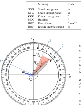
Figure 1.VISIR-1.b directional conventions on top of the compass protractor. Shown is the vessel speed through water (F), flow speed (w), vessel COG (ψe), vessel heading (ψs), flow direction (ψw),
and angle of attack through water (δ=ψs−ψe). The length of the
longer cathetus of the blue triangle is equal to the shorter cathetus of the red triangle and represents the cross-current magnitudew⊥= Fsinδ; see Eq. (7). The configuration displayed refers to a vessel course assignment (ψe=25◦) and implies a positive angle of attack
(δ=21◦) which balances the drift due to a port-bearing floww.
To keep the course constrained as per Eq. (2), it is assumed that the shipmaster can act on the rudder(s) for modifying the headinghˆuntil COG satisfies Eq. (2) and then report the rudder(s) to the midship.
2.2 Resulting kinematics
After defining the vector components of the water flow,
w= kwk ˆw=(u, v)T, (3)
and making reference to Fig. 1, the flow projections along (eˆ) and across the vehicle course (oˆ), respectively, are
wk= kwkcos(ψe−ψw)=usin(ψe)+vcos(ψe), (4a)
w⊥= kwksin(ψe−ψw)=vsin(ψe)−ucos(ψe), (4b)
where for both courseψeand flow directionψw, the nautical
or oceanographic convention (i.e. where-to direction, clock-wise from due north) is employed. Furthermore, the choice of orientation of theoˆ axis in Fig. 1 implies that a current bears to port wheneverw⊥>0.
Linear superposition Eq. (1) and the course assignment condition Eq. (2) result into two scalar equations that, upon definition of an angle of attackδ of the ship’s hull through the water (see Richardson, 1997),
δ=ψs−ψe, (5)
as the difference between the angle of vehicle heading (ψs or
heading – HDG) and the COG, read
Sg=Fcos(δ)+wk, (6a)
0= −Fsin(δ)+w⊥, (6b)
with the unknownSg being recognised as the vehicle SOG.
Remarkably, Eqs. (6a)–(6b) could also be used to determine ocean current vector w given the SOG, STW, course, and heading. As long asF is non-null,δis given by
δ=arcsinw⊥ F
, F 6=0. (7)
In the presence of waves,Fis reduced due to the wave-added resistance and can be obtained from a thrust-balance equation as in Mannarini et al. (2016a, Eq. 14). AsF is always non-negative, Eq. (7) implies that sgn(δ)=sgn(w⊥). In particu-lar, in the case of a crossfloww⊥bearing to port, a clockwise change of vehicle heading is needed for keeping course, as in the example shown in Fig. 1.
Insertingδinto Eq. (6a), SOG is obtained:
Sg=wk+ q
F2−w2
⊥. (8)
along-edge flow wk(“drag”) may instead either increase or decrease SOG. Notice that the “cross” and “along” specifica-tions refer to vessel course, differing from vessel heading by the (usually small) amount given in Eq. (7). Also it should be noted that a condition,
Sg≥0, (9)
is not guaranteed in case of a strong countercurrent. In a di-rected graph (as the one used in VISIR), a violation of Eq. (9) along a specific edge would imply that the edge is made un-available for sailing along that direction.
An equation formally identical to Eq. (8) was retrieved by Cheung (2017) in the context of flight path prediction, with wind replacing the ocean currents and plane true airspeed replacing vessel STW.
Furthermore, both Eqs. (7) and (8) hold if and only if
|w⊥| ≤F. (10)
If this is not the case, vehicle speed cannot compensate for ocean current drift. We note that Eq. (10) is satisfied even in case of a vehicle drifting along the streamlines of the flow field without any steering (F=w⊥=0). Equation (1) then reduces to dx/dt=wkeˆ, and vehicle heading is aligned with COG, or
δ=0, F =0. (11)
Finally, by taking the module of both sides of Eq. (1) and approximating the l.h.s. (left-hand side) with its finite-difference quotient (thus leading to a first-order truncation error), the graph edge weightδtis computed as
δt=δx Sg
, (12)
whereδx is the edge length. The weightsδt are then used for the computation of a time-dependent shortest path, using the same graph-search method described in Mannarini et al. (2016a) and updated in this paper in Sect. 2.4.
2.3 Graph preparation
In this section we report the procedure for ensuring that the graph used by VISIR is safe for navigational purposes. A note on use of non-regular meshes can be found in Ap-pendix C.
Due to the non-convexity of the shoreline and the pres-ence of islands, the maritime space domain is not simply connected, and thus not all graph edges correspond to naviga-ble courses. To account for this, the following graph pruning methodology is used. It starts from the observation that in a large ocean domain, most of the edges do not intersect the coastline. Thus, the procedure consists of the following three steps:
i. Retrieve the indices of edges within a small bounding box around each coastline segment.
ii. Check edges within the bounding box for intersection with the coastline.
iii. Create all edges in the selected domain, pruning just those from the previous step and intersecting the coast-line.
The first step can be performed in a constant time with re-spect to the size of the maritime domain because the graph is based on a structured grid. Furthermore, it can use a lower-resolution version of the shoreline (see Sect. 4.1.2), while the second step must use a higher-resolution.
Thus, when creating the graph, only the sea and land arcs that do not intersect the shoreline are included in the graph. When the code for track computation is then run, for each of the requested track endpoints (i.e. start and end location of the route), the nearest node on the graph is determined. This can even be a land rather then a sea node. In the subsequent step, the graph arcs are screened for the condition that the under keel clearance (UKC) is UKC=z−T >0 (Mannar-ini et al., 2016a, Eq. 44). Thus, if the start node was found on land (UKC≤0), no outgoing path from that node can be computed and VISIR quits with a warning. The coordinate of the requested endpoint must then be shifted by the VISIR user so that its next node is not on land any more. This re-quires improvements before it can be used operationally, but for the current assessment exercise, whereby the endpoints are chosen just once and then used for many computations (288 tracks per route; see Sect. 4.5), this approach is still ac-ceptable.
In VISIR-1.a graph nodes were linked only to all other nodes that can be reached via either one or two hops. In this work, a larger number of hopsνis, however, allowed. This enables the angular resolution1θto be increased up to
1θ=arctan(1/ν). (13)
Theν value is also called the “order of connectivity” of the graph (Diestel, 2005). In Mannarini et al. (2019a) the point is made that the numerical solution of the shortest path problem on a graph converges to the numerical truth asνis increased in roughly inverse proportion to graph mesh spacing1g1.
The computational cost of VISIR-1.b graph generation procedure is linear in the total number of edges (from step one of the procedure above) within all the bounding boxes around the shoreline. For a given number of nodes, the com-putation time for preparing a graph of orderνthen scales as O(ν2). More information on the scaling of the method
per-formance can be found in Appendix C. 2.4 Time interpolation of edge weights
As in VISIR-1.a, edge weights are also computed out of Eq. (12) in VISIR-1.b.
1We refer here to a regular latitude–longitude mesh with 1g
The shortest path algorithm is still derived from that of Di-jkstra, which is a deterministic and exact method (Bertsekas, 1998). The algorithm was made time-dependent under the as-sumption that no waiting times at the tail nodes are necessary, or the FIFO hypothesis (Orda and Rom, 1990). Furthermore, a new option is introduced in VISIR-1.b to conduct the time interpolation of the edge weights. Here, the edge weights are not kept constant between consecutive time steps of the input geophysical fields (currents and/or waves) but are estimated at the exact time at which the tail node is expanded by the shortest path algorithm.
In Mannarini et al. (2019a) it was shown that the effect of time interpolation can be relevant wherever the environ-mental fields rapidly change between successive time steps. This is likely the case for daily averages of the wave fields (Sect. 4.1.4), which are used for the case studies (Sect. 4) of this paper.
Orda and Rom (1990) stated that, under the FIFO hy-pothesis, the worst-case estimate of the computational per-formance is, as for the static case, O(N2), with the N
being the number of graph grid points considered2. How-ever, Foschini et al. (2014) pointed out that in the presence of time-dependent edge weights, the computational perfor-mance may degrade to become non-polynomial. The scaling of performance with time interpolation (T-interp) is further investigated in Sect. 3.2 through a few empirical tests. 2.5 Vessel modelling
The VISIR-1.b vessel propulsion and seakeeping model is the same as in VISIR-1.a, but with a minor update. It is re-viewed and updated in Sect. 2.5.1–2.5.2. Furthermore, un-der the hypothesis of constant engine orun-der telegraph (EOT), an estimate of the voyage energy efficiency is provided in Sect. 2.5.3.
2.5.1 Vessel speed in a seaway
STW together with the ocean current velocity determines SOG (Eq. 1). SOG in turn determines the edge weights in the graph representation of the kinematical problem (Eq. 12). STW depends on the vessel propulsion system (MANDiesel-Turbo, 2011) and on the energy dissipated through hydro-dynamic viscous forces, aerohydro-dynamic forces, ocean surface gravity waves, and waves generated by the vessel through the water displacement (Richardson, 1997). However it is be-yond the scope of this paper to develop a vessel propulsion and seakeeping model more realistic than that in VISIR-1.a (Mannarini et al., 2016a).
That model considered the balance of thrust and resistance at the propeller, neglecting the propeller torque equation (Tri-antafyllou and Hover, 2003). In the resistance, a term related to calm water is distinguished from a wave-added resistance.
2The performance could be improved toO(NlogN )in a
codifi-cation making use of binary heaps (Bertsekas, 1998).
The calm water term depends on a dimensionless drag coef-ficientCT, which within VISIR should have a power-law
de-pendence on vessel speed through water:CT =γq(STW)q.
For the wave-added resistance, its directional and spectral dependence is neglected, and only the peak value of the radi-ation part is considered. The latter was obtained by Alexan-dersson (2009) as a function of the vessel’s principal par-ticulars, starting from a statistical reanalysis of simulations based on the method of Gerritsma and Beukelman (1972). By only considering radiation and neglecting the diffraction term, wave-added resistance may be underestimated for long vessels with respect to the wavelength.
2.5.2 Vessel intact stability
In line with IMO guidance (IMO, 2007), VISIR also uses sea-state information to conduct a few checks of a vessel’s intact stability. In Mannarini et al. (2016a) ongoing research activity into this topic was noted. Specifically, at that time the development of “second-generation” stability criteria was proposed by Belenky et al. (2011). A recent terms of refer-ence for updating the IMO stability code (IMO, 2008) was published by the (IMO, 2018c).
At present, VISIR includes checks of intact stability re-lated to parametric roll, pure loss of stability, and surf-riding and/or broaching-to at an intermediate level between IMO (2007) and the second-generation criteria. Either intentional speed reduction (EOT<1; Table 1) or course change can be exploited by VISIR for fulfilling the stability checks (Man-narini et al., 2016a).
All vessel speeds at any location and direction (i.e. on each of theAedges) and any time (Nt time steps) are
com-puted ahead of path optimisation (Mannarini et al., 2016a, following Sect. 2.2.2 and pseudocode in Appendix A). A time-dependent Dijkstra algorithm (Mannarini et al., 2016a) can then manage all this spatially and temporally dependent information for computing the time-optimal paths. Its cor-rectness is demonstrated by comparison with the path re-sulting from the benchmark solution in a dynamic-flow field (Sect. 3.1.2; Fig. 2; Table 2). Similarly, edges that, for a given EOT, violate stability are pruned before the shortest path al-gorithm is run. Stability loss is assumed to be local in both space and time, no matter what the previous path is before the vessel sails through the edge, violating stability. Thus, the edge is pruned only for that time step ahead of path opti-misation.
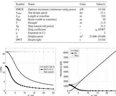
Therefore in terms of vessel stability, the sole update in VISIR-1.b is in the actual values of the vessel parameters and the parametric roll stability check. The new vessel pa-rameters are suited for modelling a container ship and are listed in Table 4. These values result in an STW dependance on significant wave height as in Fig. 4a and resistance as in Fig. 4b. For the parametric roll, the wave steepness criterion is generalised for vessels ofLwl>100 m by implementing
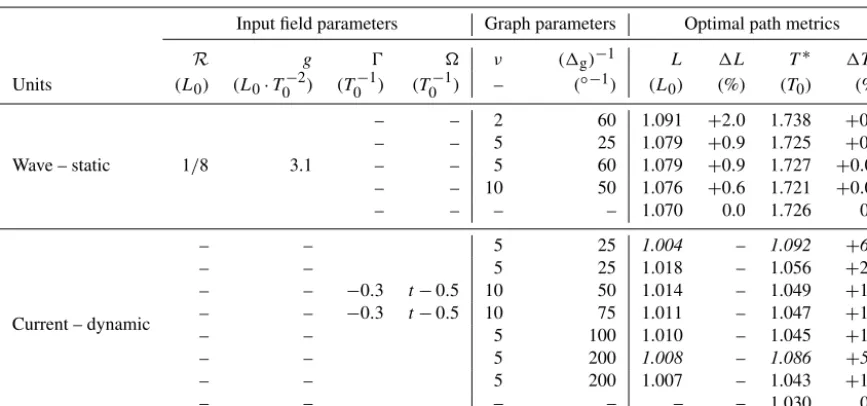
Table 2.Summary parameters of benchmark case studies (see Fig. 2). Length scaleL0set by the track endpoint distance and timescale T0=L0/Vmaxare employed throughout (Vmax=21.1 kn). Values in italics correspond to runs without time interpolation of the edge weights (see Sect. 2.4). Values in the last row of each group refer to the analytic solutions.
Input field parameters Graph parameters Optimal path metrics
R g 0 ν (1g)−1 L 1L T∗ 1T∗
Units (L0) (L0·T0−2) (T −1 0 ) (T
−1
0 ) – (
◦−1) (L
0) (%) (T0) (%)
Wave – static
– – 2 60 1.091 +2.0 1.738 +0.7
– – 5 25 1.079 +0.9 1.725 +0.3
1/8 3.1 – – 5 60 1.079 +0.9 1.727 +0.05
– – 10 50 1.076 +0.6 1.721 +0.06
– – – – 1.070 0.0 1.726 0.0
Current – dynamic
– – 5 25 1.004 – 1.092 +6.0
– – 5 25 1.018 – 1.056 +2.5
– – −0.3 t−0.5 10 50 1.014 – 1.049 +1.9
– – −0.3 t−0.5 10 75 1.011 – 1.047 +1.6
– – 5 100 1.010 – 1.045 +1.5
– – 5 200 1.008 – 1.086 +5.4
– – 5 200 1.007 – 1.043 +1.3
– – – – – – 1.030 0.0
(2011, Eq. 2.37). Thus the method of Mannarini et al. (2016a, Eq. 32) is replaced by
Hs/Lwl≥6, (14)
where the critical ratio6is given by
6=
1/20 for Lwl<100 m,
1/3·(1/5−Lwl[m]/2000) for 100 m≤Lwl<300 m,
1/60 for Lwl≥300 m.
(15)
As the stability changes are maximised for a ship length close to the wavelength (Belenky et al., 2011, Sect. 2.3.3), the 6 ratio also represents a critical wave steepness. Thus, Eq. (15) implies that it reduces at larger wavelengths, mak-ing the check on loss of stability in rough seas more severe than within the previous (VISIR-1.a) formulation.
2.5.3 Voyage energy efficiency
In this subsection the impact of track optimisation on voyage energy efficiency is estimated.
Following the Paris Agreement (UNFCCC, 2015), anthro-pogenic climate change is receiving increased attention at both international and regulatory levels. The Intergovern-mental Panel on Climate Change recently published a spe-cial report on the greenhouse gas (GHG) emission reduction pathway to limit global warming above pre-industrial levels to 1.5◦. It was noted that this would require rapid and far-reaching transitions in energy systems and transport infras-tructure (IPCC, 2018).
The third IMO GHG study estimated the share of emis-sions from international shipping in 2012 to be some 2.2 %
of the total anthropogenic CO2emissions (IMO, 2014).
Ac-cording to the EDGAR database, emissions from interna-tional shipping in 2015 were higher than the quota of two countries such as Italy and Spain put together (JRC and PBL, 2016).
In line with the United Nations Sustainable Development Goal 13 (https://sustainabledevelopment.un.org/sdg13, last access: 12 July 2019), an initial GHG reduction strategy was approved by the IMO in April 2018 (IMO, 2018b). It is lay-ered into three levels of ambition, with the second one be-ing “to reduce CO2emissions per transport work, as an
aver-age across international shipping, by at least 40 % by 2030, pursuing efforts towards 70 % by 2050, compared to 2008”. Implementation through short-term, middle-term, and long-term measures is envisaged. The short-long-term measures include the development of suitable indicators of operational energy efficiency.
The IMO previously introduced the Energy Efficiency Op-erational Indicator (EEOI) as the ratio of CO2emissions per
unit of transport work (IMO, 2009b). There are several pos-sible definitions of transport work that depend on vessel type. We have restricted our focus to a cargo vessel carrying solely containers, for which transport work is defined as deadweight (DWT) times sailed distanceL. In order to estimate the quan-tity in the numerator of EEOI, the CO2emissions are taken
to be proportional to fuel consumption (IMO, 2009b), ending with
EEOI=CF·s·P·T
DWT·L , (16)
where theCFis a conversion factor from fuel consumption to
mass of CO2emitted,sis the specific fuel consumption,P is
Figure 2.Verification of VISIR-1.b vs. benchmark solutions. Both least-distance (blue) and least-time (red) trajectories are displayed, and the tracks originate at the black star symbols.(a)A static ship velocity field as in Eq. (19) is shown; the analytical solution (branch of an inverted descent cycloid) is portrayed as a dashed black line (see Mannarini et al., 2016a, Fig. 9).(b)A time-dependent current field as in Eq. (20); the vehicle heading is portrayed as orange ar-rows. The radial sectors separated by green dashed lines refer to a sequence of time steps in the field, which are numbered in the outer sector. On the other hand, sector-mean times with a unit ofT0are given in the inner sector. Sectors nos. 3, 6, and 8 should be com-pared to Techy (2011, Fig. 12a–c). In both(a)and(b), the legend units are knots and velocity field isolines every 5 kn are displayed as dots. Parameters of the synthetic fields are given in Table 2.
inP are allowed by the VISIR algorithm (Sect. 2.5.2), while sis assumed to be a constant.
If a track is plied at a constantP (i.e. EOT=1), the emis-sions are then proportional to T, and the EEOI ratioρβ,α
of two tracks between same endpoints and sailed with same
DWT is given by ρβ,α=
EEOIβ
EEOIα
= Tβ Lβ
/Tα Lα
, (17)
where the subscripts label theβtrack being compared to the αtrack. Equation (17) shows that ρβ,α is the inverse ratio
of the average speeds along theβ andαtracks. The EEOI relative change ofβtoαtrack is then given by
1(EEOI)β,α=
EEOIβ−EEOIα
EEOIα
=ρβ,α−1. (18)
If the average speed in the β track is higher than in the α track, then −1(EEOI)β,α>0, i.e. a EEOI saving is
achieved.
Depending on the subscriptsαandβ, different types of −1(EEOI)β,α values will be computed in Sect. 4.4.4 for
analysing the benefit of the optimal tracks. A non-constant EOT is accounted for by VISIR. However, for the EOT=1 limiting case, the following general properties can be estab-lished:
i. If vessel stability checks (Sect. 2.5.1) do not lead to any diversions, the mean speed along the optimal track is never lower than along the least-distance (or geodetic) track. Thus, related EEOI savings are always non nega-tive:−1(EEOI)β,g≥0.
ii. Since currents can be either advantageous or detrimen-tal to SOG (Eq. 8), savings of the optimal tracks of cw type can have any sign with respect to optimal tracks of w type,−1(EEOI)cw,w<>0.
Predicted and recorded EEOIs for a trans-Pacific route are compared in Lu et al. (2015).
3 Verification and performance
VISIR-1.b path kinematics described in Sect. 2 are used for the numerical computation of optimal paths on graphs. In this section, an assessment of VISIR-1.b numerics is provided by means of verification vs. analytical benchmarks (Sect. 3.1) and a test of its computational performance (Sect. 3.2). 3.1 Analytical benchmarks
For the verification, VISIR-1.b includes a verification op-tion to run synthetic fields as the input, instead of those from data-assimilative geophysical models (as described in Sect. 4.1), leading to analytically known least-time trajecto-ries or brachistochrones.
3.1.1 Waves
The least-time route in the presence of waves is computed using VISIR by assuming that waves affect the speed through water of the vessel (Sect. 2.5.1). For a static wave field, this leads to an STW that is not explicitly dependent on time. This allows for the least-time path problem to be formulated in terms of a variational problem.
Analytical solutions are available for a subclass of these problems, in which STW depends on only one of the spa-tial coordinates (Morin, 2007). In particular, if speed through waterF depends on the square root of the position, as in
F =p2g(2R−y), (19)
and the initial point is aty=2R, the least-time path is given by (an arc of) a cycloid, withRandgparameters determin-ing length and acceleration, respectively (Broer, 2014; Jame-son and Vassberg, 2000). The cycloid presents a cuspid at the initial point, because along a brachistochrone, the region with F=0 has to be quit first. The remainder of the path corresponds to refraction within layers of increasing speed or decreasing wave height, according to Snell’s law.
The cycloidal benchmark was also exploited in Mannar-ini et al. (2016a), where the numerical error of VISIR-1.a in path shape and duration was ascribed to the limited angular resolution (a graph withν=2 was used).
For VISIR-1.b, we compute graphs of higher connectiv-ity (Sect. 2.3), allowing the cycloidal benchmark to be more closely approached. The results are provided in Fig. 2a and Table 2. A relative error of less than 1 ‰ in T∗ can be at-tained by only acting on graph connectivity. This improves the accuracy of VISIR-1.a by about 1 order of magnitude.
The cycloidal solution exploits the fact that a functional of the spatial coordinate is minimised under some neces-sary conditions provided by the Euler–Lagrange equations (Vratanar and Saje, 1998). The hypotheses leading to these equations are not satisfied in the more general case where the integrand of the functional explicitly depends on time. In-stead, an assessment of the VISIR solution in time-dependent waves was conducted by comparison with the numerical re-sults of an exact method based on partial differential equa-tions (Mannarini et al., 2019a). However, the verification of VISIR with time-dependent fields against an analytical benchmark is possible in the absence of waves and the pres-ence of currents, as described in Sect. 3.1.2.
3.1.2 Currents
The optimal control formalism provides the framework for computing extremals of a function, not only explicitly de-pending on spatial coordinates but also on time (Pontrya-gin et al., 1962; Bijlsma, 1975; Luenberger, 1979). As the optimal path is controlled by a group of variables, an addi-tional relation (“adjoint equation”) holds. A variant of this approach, the Bolza problem, was used for the computation
of optimal transatlantic tracks with a time-dependent STW by Bijlsma (1975). Due to topological constraints, some re-gions of the ocean are unreachable, and the method involves guessing the initial vessel course, which may hinder the im-plementation in an automated system. Another variant is the approach of Perakis and Papadakis (1989), which accounts for a delayed departure time and for passage through an inter-mediate location. However, its outcome is limited to finding only spatially local optimality conditions.
Several benchmark trajectories are provided by Techy (2011) based on Pontryagin’s minimum principle (Luen-berger, 1979), which uses vehicle heading as a control vari-able. In particular, in the presence of currents, and for a con-stant speedF relative to the flow (analogous to STW in the nautical case), an analytical relation between vehicle heading (which is the control variable) and vorticity of any (point-symmetric) current field is demonstrated. The field is given by
u=0 x− y,
v= x+0 y, (20)
where both0andmay depend on time. For the case study (Techy, 2011, Example 3), the start and endpoints are set at the side of one equilateral triangle, and the third vertex is at the flow origin (x=y=0). Finally, the duration T∗of the least-time path is retrieved through an iteration on the initial heading.
Figure 2b displays the VISIR.b solution to Eq. (20) for a case where0is a non-null constant (divergent flow) and (one-half of the vertical vorticity) linearly changes in time as per parameters of Table 2. The resulting optimal path changes its curvature, swinging on both sides of the geode-tic track, which is crossed at about one-third of its length (see Techy, 2011, Fig. 12). The elongation of the swinging is quite small, with the optimal path differing from the geode-tic by less than 1 % in length. This poses a challenge to the numerical solver on the graph, as many accurate course vari-ations are required over a short distance. Thus, it is not sur-prising to find that the graph mesh spacing1gis more
crit-ical for achieving convergence than the graph order of con-nectivityν. However, this only holds if a time interpolation of edge weights (Sect. 2.4) is used. Otherwise, no signifi-cant improvements inT∗can be achieved (see Table 2). With VISIR-1.b, a minimum error of about 1.3 % inT∗is obtained for the graphs used.
3.2 Computational performance
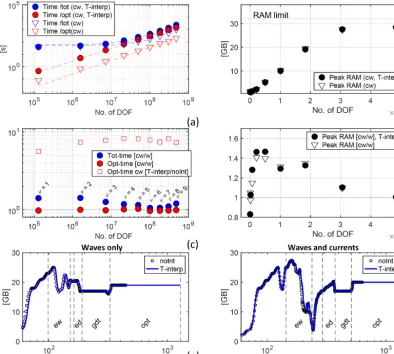
RAM: 32 GB 1600 MHz DDR3). The results are displayed in Fig. 3. Here, the number of degrees of freedom (DOFs) of a VISIR job is given by the productNtAof the numberNt
of time steps (i.e. days) and the numberAof graph edges.A in turn depends on the number of grid points N comprised within the geographical region selected and on the orderνof the graph. Jobs with DOFs varying over more than 4 decades are considered, corresponding to graph ordersν∈ {1,9}. 3.2.1 CPU time
Figure 3a displays both the cost of computing only the op-timal track via the shortest path algorithm and the total job cost from its submission to the saving of the results (ren-dering excluded). Cases without and with time interpolation of the edge weights are distinguished (Sect. 2.4). The CPU time for the optimal track increases almost nearly linearly with the DOF. Below the 107 DOF, a minimum delay of about 1 min can be noticed in the total job cost, which is due to input–output operations. All fitted parameters are re-ported in Table 3. Asymptotically, it is found that the VISIR time-dependent optimal path algorithm (with time interpola-tion being active) can be run at a cost of less than 3 µs per DOF. For comparisons to other ship-routing models, see Ap-pendix D.
In any two-dimensional regular mesh, the number N of graph grid nodes scales quadratically with the inverse mesh resolution, N∼(1/1g)2. For the series of experiments in
Fig. 3, we variedνas 1/1g. When taken together, these two
effects result in
DOF=A·Nt∼ν2N∼(1/1g)4=O(N2). (21)
Thus, the empirically retrieved linearity of CPU time with the DOF corresponds to a quadratic dependence inN. This is in fact the expected worst-case performance of Dijkstra’s algorithm (Bertsekas, 1998). In the presence of binary heaps, such an estimate can be reduced toNlogN. This will be con-sidered in future VISIR versions.
Without time interpolation, the optimal path algorithm is about 8 times faster (Fig. 3c). Furthermore, in Fig. 3c the computational overhead from the use of currents besides waves is assessed. There is no overhead for the shortest path computations (red circles), as they use a set of edge weights of the same size for both cases in the inputs. Instead, edge weight values are determined through the specific environ-mental fields used (waves alone or also currents). Thus, the preparation of the denominator in Eq. (12) causes an over-head for the total job (blue circles), which is up to 30 % for the sampled DOF range. Starting from ν=8, a rise in the overhead is observed. To understand its origin, the RAM al-location is investigated in the following section.
3.2.2 RAM allocation
Figure 3b shows that peak RAM increases to about 3× 10⁸DOF, where it saturates. Here, the computer’s physical memory limit is approached, which leads to swapping and to a degradation of performance, as already observed in Fig. 3c. This is even more apparent in Fig. 3d, where the ratio of peak RAM for the cw- to w-type computations is displayed. Peak RAM allocation occurs – for large enough jobs – during edge weights preparation, prior to the run of the shortest path algorithm (see ew and opt phases in Fig. 3e and f). There is up to 50 % extra RAM that needs to be allocated if ocean cur-rents are considered. In fact, five environmental scalar fields must be considered (significant wave height, direction, peak period, and zonal and meridional current), but the latter two are not used in the w-type computations. Thus, apart from noise being below 1×10⁸DOF, a drop of the cw-to-w peak RAM ratio is recorded, as the allocation for the cw case satu-rates, while, for the w case, it is still significantly lower than such a limit and can grow further. Thus, from Fig. 3d it is pos-sible to define a “computational efficiency region” for VISIR jobs with a DOF lower than the one leading to the drop ob-served in Fig. 3d. The computations in Sect. 4 are performed on a cluster with a RAM of 64 GB, which can operate in its efficiency region even for larger DOF values.
To further clarify the memory space requirements of VISIR, we focussed on its shortest path algorithm and col-lected and analysed additional datasets, as described below. These consist of the following:
d1 time series of RAM allocation of the VISIR MATLAB
job3,
d2 stopwatch timer readings at specific VISIR processing
phases4.
Thed2 dataset is then temporally offset by matching the
end of the d1 dataset. Finally, the resulting d2 data are
smoothed by thinning, which results in the plots displayed in Fig. 3e–f below.
For each graph’s angular resolution (indexed byν param-eter), the time series exhibit different relative importance (both in terms of duration and RAM allocation) of the var-ious processing phases. However, thed1andd2datasets
con-firm that, for 6≤ν≤9, the peak RAM is allocated during the edge weight computation (ew phase). Furthermore, the shortest path algorithm is run twice: in its static version (Di-jkstra, 1959) for the computation of the geodetic track and in a time-dependent version for the optimal track (Mannarini et al., 2016a). The latter requires the edge delays atNt time
steps in the input, and this justifies the uphill RAM step be-tween these two phases. Finally, Fig. 3e–f proves that time
3The following shell command is used: top | grep
MATLAB >> RAM-timeseries.txt.
Figure 3. (a)CPU time for the total VISIR job (blue markers) and for just the computation of the time-dependent shortest path (red markers). Only the cw case is considered. Dashed lines are fits of the model in Table 3.(b)Peak RAM allocation during the computing jobs of(a), with a reference line at the total installed RAM.(c)Ratio of CPU times between the cw and w cases and (just for optimal path) with and without time interpolation (T-interp).(d)Ratio of peak RAM allocation of the cw- to w-type jobs. For panels(a),(b), and(d), both cases are with (filled markers) and without (empty markers) time interpolation. The DOF of the time-dependent shortest path problems is displayed on the horizontal axis.(e, f)Time series of RAM memory allocation during VISIR execution for w- and cw-type jobs, respectively. Black circles (blue lines) refer to runs without (with) time interpolation of edge weights. Vertical dashed lines separate the main phases of the processing. Both panels refer to theν=8 case of(a–d). The processing phase labels are as follows: ew (computation of edge-averaged fields), ed (edge delays), gdt (geodetic track), and opt (optimal track).
Table 3.Fit parameters for the data displayed in Fig. 3a. The fit model isa·xb+c. For the optimal path data,cparameter is not fitted.
No T-interp With T-interp
Units Optimal path Total job Optimal path Total job
a s 9.9×10⁻⁸ 4.7×10⁻¹⁰ 2.6×10⁻⁶ 1.2×10⁻⁷
b – 1.07 1.42 1.01 1.18
c s – 52 – 60
interpolation does not affect RAM allocation but solely CPU time.
4 Case studies
In this section, the capacity of VISIR-1.b to deal with both dynamic flows and sea-state fields in realistic settings is demonstrated using the ocean current and wave analysis fields from data-assimilative ocean models.
Section 4.1 presents the environmental fields used for the computations. A documentation of the principal VISIR model settings is presented in Sect. 4.2. A description of the results on individual tracks of a given departure date is given in Sect. 4.3. The analysis of their seasonal variability within a calendar year is conducted in Sect. 4.4, and the extension of such analysis to several routes in the Atlantic Ocean is provided in Sect. 4.5.
4.1 Environmental fields
VISIR-1.b uses both static and dynamic environmental fields obtained from official European and US providers. The static environmental datasets are of the bathymetry and shoreline. The dynamic datasets are of the waves and ocean currents. The specific fields used are described in the following sub-sections.
4.1.1 Bathymetry
The General Bathymetric Chart of the Oceans (GEBCO) 2014 bathymetric database (https://www.gebco.net/data_ and_products/gridded_bathymetry_data/, last access: 12 July 2019; Weatherall et al., 2015) is used in VISIR-1.b. Its spatial resolution is 30 arcsec or 0.5 nmi in the meridional direction.
4.1.2 Shoreline
The Global Self-consistent, Hierarchical, High-resolution Geography Database (GSHHG; https://www.ngdc.noaa.gov/ mgg/shorelines/, last access: 12 July 2019) of the NOAA (Wessel and Smith, 1996) is used in VISIR-1.b. There are five versions (c, l, i, h, and f) of the database, with a res-olution of about 200 m in the best case. Depending on the geographic domain, VISIR-1.b uses different versions of the GSHHG for the generation of the graph (Sect. 2.3). This lim-its the generation time in the case of jagged coastlines, such as in archipelagic domains.
4.1.3 Wind
Meteorological fields have not as of yet been used for com-puting VISIR-1.b tracks. Surface wind fields have only been used in VISIR-1.a for sailboats (Mannarini et al., 2015). Wind also directly affects motor vessels through an added aerodynamic resistance and a heeling moment, which are
mainly significant for vessels with a large superstructure, such as passenger ships (Fujiwara et al., 2006). This will be considered in future VISIR developments. We have only used an NOAA Ocean Prediction Center review of marine weather (https://www.vos.noaa.gov/, last access: 12 July 2019) for describing the synoptic situation affecting the ocean state during the periods of the case study of Sect. 4.3. An archive of surface analysis maps (http://www.wetterzentrale.de, last access: 12 July 2019) is also considered.
4.1.4 Waves
Wave analyses are obtained through Copernicus Marine Environment Monitoring Service (CMEMS; http://marine. copernicus.eu/, last access: 12 July 2019) from the opera-tional global ocean analysis and forecast system of Météo-France, based on the third-generation wave model MFWAM (Aouf and Lefevre, 2013).
This uses the optimal interpolation of significant wave height from Jason-2 and Jason-3 and SARAL and CryoSat-2 altimeters. The model also takes into account the ef-fect of currents on waves (Komen et al., 1996; Clementi et al., 2017). Thus, surface currents from the corresponding CMEMS product (see Sect. 4.1.5) are employed and used to force the wave model daily. The currents modulate wave energy and also cause a refraction of the wave propagation. The wave spectrum is discretised into 24 directions and 30 frequencies in the 0.035–0.58 Hz range. Classically, this is the realm of ocean surface gravity waves (Munk, 1951). The vessel intact stability constraints used in VISIR (Sect. 2.5.2) set a timescale given by the vessel natural roll period (usually up to about 20 s or more than 0.05 Hz).
The spatial resolution is 1/12◦(i.e. 5 nmi in the meridional direction). Three-hourly instantaneous fields of integrated wave parameters from the total spectrum (spectral significant wave height, mean wave direction, and wave period at the spectral peak) are averaged in a preprocessing stage based on “cdo dayavg” (https://code.mpimet.mpg.de/projects/cdo/, last access: 12 July 2019) into daily fields. Neither Stoke’s drift nor the partitions (wind wave, primary swell wave, and secondary swell wave) are used as of yet in VISIR. Due to a much larger fetch, the impact of the swell is estimated to be more significant in the South than in the North Atlantic Ocean (Hinwood et al., 1982).
The wave dataset name is
GLOBAL_ANALYSIS_FORECAST_WAV_001_027 (http://cmems-resources.cls.fr/documents/PUM/
4.1.5 Currents
Ocean currents are obtained through CMEMS from the op-erational Mercator global ocean analysis and forecast system based on the NEMO v3.1 ocean model (Madec, 2008).
This uses the SAM2 (SEEK Kernel) scheme for assimi-lating the sea level anomaly, sea surface temperature, mean dynamic topography (CNES-CLS13), and more. The spatial resolution is 1/12◦ (i.e. 5 nmi in the meridional direction). Daily analyses of surface fields are used in VISIR-1.b.
The dataset name is GLOBAL_ANALYSIS_FORECAST _PHY_001_024 (http://cmems-resources.cls.fr/documents/ PUM/CMEMS-GLO-PUM-001-024.pdf, last access: 12 July 2019), and the product validation is provided by a companion document (http://cmems-resources.cls.fr/ documents/QUID/CMEMS-GLO-QUID-001-024.pdf, last access: 12 July 2019). The datasets were downloaded from CMEMS at least 14 d after their date of validity, ensuring that the best analyses were used.
4.2 VISIR settings
For the results shown in this section, optimal tracks are com-puted on a graph with the order of connectivity ofν=8 (see Sect. 2.3) and mesh spacing1g=1/8◦. These graph
resolu-tion parameters are chosen to strike a compromise between track accuracy (i.e. spatial and angular resolution) and com-putational cost of the numerical jobs (see the discussion in Sect. 3.2). The computations refer to a container ship, and the parameters are reported in Table 4. The resulting vessel’s performance in waves is summarised in Fig. 4.
4.3 Individual tracks
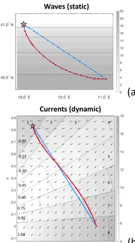
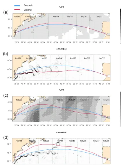
We first consider a transatlantic crossing in the North Atlantic Ocean, located between Norfolk (USNFK), at the mouth of the Chesapeake Bay (37◦02.50N, 76◦04.20W), and Algeci-ras (ESALG), just past the Strait of Gibraltar (36◦07.60N, 5◦24.90W). Both east- and westbound tracks are considered (Fig. 5).
First of all, we note that the geodetic (or least-distance) track is bent northwards, as it is to be expected from an arc of GC of the Northern Hemisphere on an equi-rectangular pro-jection. The track is piecewise linear, and its northern edge is flattened due to the finite angular resolution of the graph: 1θ≈7.1◦from Eq. (13). However, as Table 5 reports, the error in the length of the geodetic route made by VISIR is only a few per mil. This is comparable to the accuracy of the function for the computation of distances on the sphere (used in VISIR) compared to the ellipsoidal datum (which is more accurate but slower).
For these tracks, meteo-marine conditions are first intro-duced (Sect. 4.3.1), and track spatial and dynamical fea-tures are then discussed in Sect. 4.3.2 along with the
im-pact on vessel stability in Sect. 4.3.3 and their base metrics in Sect. 4.3.4.
4.3.1 Meteo-marine conditions
The synoptic situation in the North Atlantic during the week following 21 June 2017 (departure date for the eastbound track) was dominated by the Azores High blocking descent of subpolar lows to the middle latitudes. This led to relatively calm ocean conditions (significant wave heightHs<5 m) for
most of the region involved in the Norfolk–Algeciras cross-ing.
In the week following 16 February 2017 (departure date for the westbound track) a low with storm-force winds that formed near (41◦N, 52◦W) was observed, which then moved N, influencing wave direction on the 19 and 20 February. On 22 February another storm with waves ofHs>8 m
devel-oped (37◦N, 58◦W).
In terms of the currents, we note that the eastern edge of the crossing is N of Cape Hatteras and, thus, N of the GS branch known as the Florida Current (Tomczak and Godfrey, 1994).
4.3.2 Track spatial and dynamical features
The topological and kinematical features of the optimal tracks of the case study are discussed in this subsection. Track topology
Four different solutions for the optimal tracks of the USNFK–ESALG route are given in Fig. 5 (red lines).
For the eastbound voyage, when only considering waves (w type; Fig. 5a) the optimal track is quite close to the geode-tic track. This is due to the absence of waves of relevant height along the path during the crossing (about 8 d; see Table 5). Discontinuities are seen between significant wave height fields at consecutive time steps (vertical stripes sepa-rated by dashed lines). This is enhanced by the daily averag-ing of the original 3-hourly fields (see Sect. 4.1.4).
When the optimal track is computed for the same depar-ture date and direction but also considers ocean currents too (cw type), the solution is significantly modified (Fig. 5b). A diversion S of the geodetic track is computed by VISIR-1.b. This is instrumental in exploiting advection by the GS through velocity composition (Eq. 8). Despite being longer in terms of sailed miles, this track is faster than the geodetic track (Table 5). A closer look at Fig. 5b reveals that the opti-mal track averages between the locations of opposite mean-ders of the first six oscillations of the GS proper, at 72–63◦W. Subsequent meanders, which are prone to extrude filaments (and are thus more stretched in the meridional direction), are followed increasingly loosely by the optimal track.
Table 4. Database of vessel propulsion parameters and principal particulars used in this work. The values of1(ballast minus scantling range) and the maximum cargo capacity (2500 TEUs – 20 ft equivalent units) are not used in the computations and are provided just for the sake of reference.
Symbol Name Units Value(s)
SMCR Optimal maximum continuous rating power kW 19 164
Vmax Top design speed kn 21.1
Lwl Length at waterline m 210
BWL Beam (width at waterline) m 30
T Draught m 11.5
TR Ship natural roll period s 21.2
CT Drag coefficient – γqSTWq
q Exponent inCT – 2
1 Displacement m3 21 600–45 600
DWT Deadweight t 33 434
Figure 4.Vessel response functions for the parameters given in Table 4.(a)STW at a constant engine throttle vs. significant wave height Hs. Both EOT=100 % (solid line) and EOT=10 % (line and dots) are displayed.(b)Calm waterRc, wave-added resistanceRaw, and their sumRtotas functions ofHs.
geodetic track, because it skips both the storm in the north-eastern Atlantic at1t=1–4 d since departure and the storm developing at1t=6 d at the latitude of the arrival harbour.
The optimal track for the same departure date and direc-tion but different cw type (Fig. 5d) leads to yet another solu-tion with respect to the w-type track. It sails N of the geode-tic at all times. The speed loss due to the encounter with the storm at 1t=2–3 d is balanced by the speed gains due to a meander of the North Atlantic current encountered at 1t≈4 d at 44◦N and by the benefit of sailing slightly fur-ther away from the rough sea than the corresponding w-type track at1t=5–6 d.
Tracks kinematics
To gain a deeper insight into the results, in Fig. 6, a few kine-matical variables are extracted along both the optimal and geodetic tracks for both cw and w cases.
Starting from the eastbound route (Fig. 6a), the SOG of the cw optimal track differs greatly from the corresponding geodetic track. SOG gains by up to more than 4 kn are ex-perienced in the first half of the path due to the GS. During the final part of the navigation (1t≈6.5 d), an SOG>22 kn peak appears to be shifted in both tracks. This is the signature of the Atlantic jet past Gibraltar, which is encountered about 5 h earlier along the optimal track (see bottom of Fig. 6c). Instead, the SOG does not appreciably differ when w-type optimal and geodetic tracks are compared. This is consistent with the spatial pattern seen in Fig. 5a.
Figure 5.Geodetic (blue) and optimal tracks (red) for the USNFK–ESALG route in the presence of different environmental forcings and departure dates: panels(a)and(c)are of w type,Hsis displayed as shading, and wave direction is displayed as white arrows. Panels(b)and
(d)are of cw type, current magnitude is displayed as shading, and its direction is displayed as white arrows. Departure date is 21 June for(a)
Figure 6.Along-route information for both the eastbound(a, c, e)and westbound(b, d, f)crossings of Fig. 5. The first row(a, b)displays the SOG for both optimal and geodetic tracks for both w and cw cases; the black dotted line isVmaxfrom Table 4. The second row(c, d)
displays thewkcomponent of the ocean flow, as computed from Eq. (4a). The third row(e, f)displays the angle of attackδfrom Eq. (5). The maximum ROT ofδis 0.8 and 0.5◦min−1for the east- and westbound track, respectively.
confirmed as enabling the larger SOG in the second part of the crossing.
In Fig. 6c–d the ocean flow component wk along vessel course (Eq. 4a) is displayed. This quantity, together with its normal counterpartw⊥, determines, through Eq. (8), the value of SOG. The difference between the optimal and the geodetic tracks is noticeable for both east- and westbound navigation. In Fig. 6c it can be seen that the algorithm man-ages to encounter a wk that is nearly always positive (i.e. along the course), which even exceeds 4 kn at the end of the first day. It is apparent that the same wkoscillations are re-trieved in the SOG line chart of Fig. 6a for 1t <3 d and at the1t≈6.5 d peak. For westbound navigation,wkis mainly positive (apart from the initial impact of the Atlantic jet
be-fore Gibraltar is passed) along the optimal track and is mainly negative along the geodetic track, which sails against the GS. At1t=4 d a NW-bound meander of the North Atlantic cur-rent is encountered, with a positive drag of up to 1.5 kn.
Finally, the angle of attack δ needed for balancing the crossfloww⊥(Eq. 5) is displayed in Fig. 6e–f. The track av-erage ofδis nearly zero, its maximum value is of the order of 10◦, and its amplitude is larger wherever|w
k|is larger. The oscillations ofδ with a larger elongation are a signature of the crossing of strong meanders, as seen in the first half of Fig. 6e and at1t=4 d in Fig. 6f.
is if the heading fluctuations corresponding to the δsignals in Fig. 6e–f are compliant with vessel manoeuvrability. The maximum module of the rate of turn (ROT) of HDG is found to be 2.9◦min−1for the eastbound track and 1.5◦min−1for the westbound track of cw type. These values are compa-rable to the IMO prescribed accuracy of 1.0◦min−1for on-board ROT Indicators (IMO, 1983). Thus, heading fluctua-tions computed by VISIR-1.b for this route should be feasi-ble with respect to manoeuvrability.
4.3.3 Safety of navigation
The stability constraints given in Sect. 2.5.2 were checked. However, some of them did not result in any graph edge pruning during the actual transatlantic crossing of the ves-sel under consideration (see parameters in Table 4). In fact, pure loss of stability was not realised, as the threshold condi-tion of the significant wave height of Mannarini et al. (2016a, Eq. 36) was not reached. Surf-riding and/or broaching-to was not activated due to the condition that the Froude number was never larger than the critical number for the wave steep-ness encountered (Mannarini et al., 2016a, Eqs. 42–43). By using the generalisation discussed in Sect. 2.5.2, parametric roll could instead occur for the present vessel parameters and the North Atlantic wave climate.
In addition, on this specific route and these departure dates, the voluntary speed reduction (Sect. 2.5.2) was not found to be activated by the algorithm. This means that the tracks are sailed at a constantP and that the CO2emissions
are linearly proportional to the sailing timeT∗(Sect. 2.5.3). Instead, for other routes in the Atlantic, this is not always the case (see Table 7).
Furthermore, all time-dependent edge weights along the optimal tracks fulfil the FIFO hypothesis (Sect. 2.4).
4.3.4 Track metrics
Two simple metrics for summarising the kinematics of a track are proposed here: the optimal track duration T∗and the corresponding length L (not a starred symbol, as this length is not the object of the optimisation). For the geode-tic tracks, optimisation is instead performed on length L∗, and, unless safety constraints play a role in the actual opti-mal track, the corresponding durationT is higher thanT∗.
L is sensitive to the geometrical level of the track diver-sions, whileT∗ reflects their kinematical impact. Such key metrics are reported in detail for both the geodetic and opti-mal tracks of both the east- and westbound crossings in Ta-ble 5. The data also allow us to distinguish the quantitative role of waves and currents and the level of the track duration gains. For example, it is seen that both east- and westbound tracks lead to time savings∼3 % with respect to the geodetic track. However, for the former, such a saving is mainly due to the exploitation of currents, while the latter is due to waves.
Concerning time gains, it is important to specify whether they refer to the geodetic track (1Tg) or to an optimal track
computed in the presence of waves only (1Tw). Here, we
observe that both Lo and McCord (1995) and Chang et al. (2013), not using waves, only consider1Tg. In addition, the
model region chosen for their track optimisation almost co-incides with the domain where the western boundary current under consideration is at its strongest. This is different from the case study presented in this section, which also entails the eastern part of the ocean, where the influence of the western boundary current is less noticeable. Thus, the1Tggains due
to currents reported in Table 5 are lower than the results in the literature, although they are possibly more realistic when referring to full transatlantic crossings.
4.4 Track seasonal variability
In this subsection we consider the extent to which the sea-sonal variability in the ocean state and circulation affects the variability in the optimal track of a given transatlantic cross-ing.
In order to address it, VISIR-1.b computations are con-ducted for departure dates spanning the whole calendar year 2017. Departures on six dates (1st, 6th, 11th, 16th, 21st, and 26th) in each month are considered, resulting in 72 dates per year. This is aimed at considering the decorrelation of the ocean current fields after a Lagrangian eddy timescale of about 5 d (Lumpkin et al., 2002). As waves are mainly driven by winds, whose velocity is 1 order of magnitude larger than ocean velocities, the timescale for the decorrelation of the ocean state is expected to be even shorter.
To analyse the massive data resulting from these compu-tations, four levels of analysis are considered: spatial vari-ability in the tracks (Sect. 4.4.1), their kinematic variabil-ity (Sect. 4.4.2), the distribution of durationT∗ and length L, (Sect. 4.4.3), and the impact on voyage energy efficiency (EEOI; Sect. 4.4.4).
4.4.1 Spatial variability
A direct visualisation of the annual variability in the track topology is shown in Fig. 7.
Each panel displays a bundle of trajectories relative to the 72 departure dates. The extent of the diversions makes it clear that the case study of Sect. 4.3 is not even extreme. Instead, for both east- and westbound tracks, the summer and autumn tracks are closest to the GC track because in the North At-lantic Ocean, wave heights tend to be smaller in these sea-sons, and consequently, both vessel speed losses and relative kinematic benefits from diversions are smaller.
Some tracks are found to sail quite far inshore towards the Canadian coast, and for this we refer to a related comment in Sect. 4.5.4.
vicin-Figure 7.Route tracks of the same transatlantic crossing of Fig. 5 during the calendar year 2017. Panels(a)and(b)refer to w type;(c)and
(d)refer to cw-type tracks. Both east- (left) and westbound tracks (right) are shown. The geodetic route is displayed as a black dashed line. Animations of the panels are available at https://av.tib.eu/series/560/gmdd+18 (last access: 12 July 2019). For this and other routes, see also the Supplement.
ity of the GS proper (W of 67◦W). On a few dates (mainly in winter and spring) this is not the case, as storm systems happen to cross the location of the GS. For the westbound tracks, also accounting for currents only adds a small pertur-bation to the wave-only tracks without dramatically changing their topology.
It should be stressed that the computed spatial variabil-ity depends heavily on how ship energy loss in waves is parametrised (see Sect. 2.5.1). Wave-added resistance deter-mines vessel STW for any given sea state and thus how prof-itable a diversion to avoid speed loss is.
4.4.2 Evolution lines
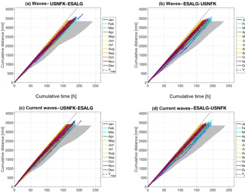
While the paths of the tracks displayed in Fig. 7 convey the information about the spatial variability and its seasonal dependence, they fail to provide information about vessel kinematics along the tracks. Thus, an alternative visualisa-tion is proposed in Fig. 8. Following a practice used in track anomaly detection (Zor and Kittler, 2017), cumulative sailed distance is displayed vs. time elapsed since departure. Thus, the slower parts of each path result in a smaller slope for corresponding segments of the track “evolution line”. It can be seen that such slow segments are more frequent in
win-ter months and in the middle of the crossing, particularly for westbound tracks, due to larger speed losses in waves.
Furthermore, in the presence of currents, the slope can ex-ceed that relative to navigation at SOG equal to the maximum STW. This is due to the speed superposition per Eq. (8) and is apparent for some of the summer tracks in the panel relating to the eastbound tracks (Fig. 8c).
Finally, the envelope of the evolution lines along the geodetic tracks is displayed as a grey shaded area. This re-veals the kinematical benefit of the optimal tracks, as they can be sailed at an higher SOG (coloured dots are generally left of the grey areas), resulting in shorter voyage durations. 4.4.3 Scatter plots
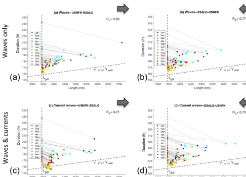
To reduce and better analyse the information contained in Fig. 8, the compound metricsT∗andLcan be used, which are reported in a Cartesian plane in Fig. 9.
Such a plane contains a strictly forbidden region, left of L=LGC, which is the length (on the graph) of the GC arc
Figure 8.Evolution lines for the tracks in Fig. 7: cumulative sailed distance is displayed vs. time elapsed since departure. Each optimal track is displayed with a coloured dot referring to the month of departure as in the legend. The envelope of the geodetic trajectories is shaded in grey. The dashed line refers to sailing atVmax.
and the region below this line corresponds to tracks sailed at an average speed higher thanVmax.
We first focus on eastbound tracks. The distribution for w-type tracks is given in Fig. 9a. As expected, they are all com-prised within the region above the T∗=L/Vmax line. This
is due to involuntary speed loss in a seaway, which reduces the average speed to less thanVmax. When currents are also
considered (Fig. 9c), the tracks can be faster, and for east-bound navigation, some of them even attain the region where the average SOG is larger thanVmax. This generally occurs
for summer tracks, which experience a lower speed loss in waves.
For the westbound tracks (Fig. 9b–d), the general picture differs in terms of the following features: the region where the average vessel SOG is larger thanVmaxis never attained,
and the distribution in the (L, T∗) plane roughly maintains its pattern among the w- and cw-type results.
These findings are also mirrored in Pearson’s correlation coefficientRP betweenT∗ andL. While for the westbound
tracksRPis nearly unchanged (Fig. 9b–d), it decreases
sub-stantially between Fig. 9a and c. Most eastbound tracks, in-dependently of their duration, require a significant diversion to exploit the GS proper. This in turn reduces the correlation betweenT∗andL.
The dots relative to the tracks selected for the featured analysis of Sect. 4.3 are seen as circles in Fig. 9. For the eastbound crossing, a transition into the efficiency region is seen when comparing the w-to the cw-tracks.
4.4.4 EEOI savings
Figure 9. Distribution of optimal sailing timeT∗ vs. lengthL of the tracks of Fig. 7. For the geodetic tracks,L=Lgdtis a constant. Corresponding optimal track dots (L, T∗) are joined by a light dotted line. The slanted dashed line has a slopeVmax−1. Tracks for w-type(a,
b)and cw-type optimisation(c, d), and for both east- and westbound directions, are displayed. Dots of the tracks analysed in Sect. 4.3 are outlined in black. Pearson’s correlation coefficientRPbetweenT∗andLis printed in the top right corner of each panel.
In reference to Sect. 2.5.3, specific fuel consumptionsis taken to be a constant, while engine brake powerPis allowed to vary as EOT is selected by the optimal routing algorithm (see Sect. 2.5.2).
With the notation of Eq. (18), EEOI savings of the tracks considering both ocean currents and waves (β=cw) are computed with respect to either the geodetic track (α=g; Fig. 10a–b) or the wave-optimal tracks (α=w; Fig. 10c–d). For the eastbound route, −1(EEOI)cw,g exhibits a clear
seasonal cycle, with a peak of the monthly mean value in winter. However, the winter intra-monthly variability ex-ceeds the amplitude of the seasonal cycle. For the westbound route, these trends are still observed, but both the seasonal cycle and the intra-monthly variability are less regular.
Furthermore, in Fig. 10c–d the monthly mean value of −1(EEOI)cw,wis found to be larger for the eastbound route,
as it can benefit from advection by the GS. Peak values of −1(EEOI)cw,w are found in summer months, when the
ocean state is calmer, and thus the relative contribution of currents is the prevalent one.
Thus, the magnitude and location of the GS is critical for voyage energy efficiency along this route in summer. In this respect, Minobe et al. (2010) found, from satellite altimetry data, that the seasonal cycle of the geostrophic component of the GS is weak both in terms of meridional position and near-surface velocity. The simulations of Kang et al. (2016) instead show a seasonal cycle of the mean kinetic energy of the GS proper, with a relative maximum during summer. Berline et al. (2006) analysed the GS latitudinal position at 75–50◦W from model reanalyses and found that inter-annual and seasonal variability dominates upstream and downstream of 65◦W, respectively.
4.5 Ocean-wide statistics