ABSTRACT
ENGELSONE, ANNA. Direct Transcription Methods in Optimal Control: Theory and Practice. (Under the direction of Stephen Campbell)
In optimal control, as in many other disciplines, individuals developing the theory and those applying it to real life problems do not always see eye to eye. Some results developed by theoreticians have very limited practical value, while other useful results may be unknown to practitioners or incorrectly interpreted. This work aims to bridge the gap between these two groups by presenting theoretical results in a way that will be useful to practitioners. We concentrate specifically on convergence results relating to a class of methods known as direct transcription, where the entire optimal control problem is discretized, in our case using a Runge-Kutta method, to form a nonlinear program.
For unconstrained problems, we present several convergence results, then give an original result that demonstrates that practically designed optimal control software will be unable to attain theoretically possible convergence order in most cases. We present a practical solution to this problem that is currently being implemented in an industrial software package.
DIRECT TRANSCRIPTION METHODS IN OPTIMAL
CONTROL: THEORY AND PRACTICE
by
Anna Engelsone
a dissertation submitted to the graduate faculty of north carolina state university
in partial fulfillment of the requirements for the degree of
doctor of philosophy
operations research
raleigh,north carolina May 2006
approved by:
Dr. Stephen L. Campbell Dr. Ralph Smith
chair of advisory committee
Biography
Acknowledgements
The research presented here was performed between 2002 and 2006 under the expert guidance of Dr. Stephen Campbell of NCSU and with frequent input from Dr. John Betts of the Boeing Company. Financial support was provided in part by NSF Grants DMS-0101802, DMS-020695, DMS-0404842, and ECS-0114095.
I would like to thank the committee members, Dr. Campbell, Dr. Gremaud, Dr. Kelley and Dr. Smith for taking time out of their busy schedules to read and evaluate this work.
A big thank you to all participants of the Numerical Analysis seminar, student and faculty alike, for their many valuable comments on my research and presentations over the past three years.
Many thanks to all the helpful staff at the Mathematics and Operations Research departments. Your contributions to the well-being and sanity of faculty, students and anyone else who comes to you for help cannot be overestimated.
Table of Contents
List of Tables vi
List of Figures vii
1 Definitions 1
1.1 Example of a Control Problem . . . 1
1.2 Standard Form and Alternative Formulations . . . 3
1.3 Optimality Conditions . . . 5
1.4 Methods of Solution . . . 7
1.5 Convergence and Discretizations . . . 9
1.6 Computation . . . 12
2 Unconstrained Problems 14 2.1 Overview . . . 14
2.2 Multiplier Convergence . . . 21
2.2.1 New Theoretical Result . . . 21
2.2.2 Numerical Example . . . 23
2.3 Open Questions . . . 29
2.4 Proofs . . . 34
2.4.1 Proof of Theorem 2.3 . . . 34
2.4.2 Proof of Theorem 2.6 . . . 35
3 Equality Constrained Problems 52 3.1 Overview . . . 52
3.2 The Virtual Index . . . 54
3.2.1 Theoretical Results . . . 54
3.2.2 Example 1: Time-Invariant Transformation . . . 59
4 Inequality Constrained Problems 74
4.1 Overview . . . 74
4.2 Virtual Boundary Arcs . . . 84
4.2.1 The Heat Equation Problem . . . 84
4.2.2 Numerical Results . . . 86
4.2.3 Discussion . . . 94
4.2.4 Example Problem . . . 96
4.2.5 Theoretical Result . . . 102
4.3 Open Questions: Initialization . . . 105
4.3.1 Monitor Functions . . . 105
4.3.2 Order Reduction . . . 107
5 Summary of Contributions 111
6 Index 116
List of Tables
1.1 Order of Runge-Kutta discretization as an integrator. . . 11
2.1 Order of Runge-Kutta discretization for optimal control. . . 18
2.2 −log2 of uncompressed TR error to gridpoint values of x, y, λ. . . 26
2.3 −log2 of compressed TR error to gridpoint values of x, y, λ. . . 26
2.4 −log2 of compressed TR error in λ: at gridpoint, at midpoint, inter-polated at gridpoint. . . 26
2.5 −log2 of compressed TR error in y: inside gridpoints and endpoints. . 27
2.6 −log2 of RK4 error to gridpoint values of x, y, λ. . . 27
2.7 −log2 of HS-RK (Butcher array) error to gridpoint values of x, y, λ. . 30
2.8 −log2 of HS-Compressed error to gridpoint values of x, y, λ. . . 31
List of Figures
1.1 The Trolley Control System. . . 2
2.1 Example problem solved with TR. Graph ofy∗−yfor N = 10,20,40,80. 25 2.2 Example problem solved with RK4. Graph of y∗−y for N = 5,10,20. 28 2.3 Example problem solved with HS. Graph ofy∗−y for N = 5,10,20. . 31
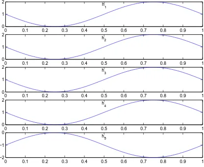
3.1 Functions hi =±(sin(2πt)−1) for Example 1. (i= 1 is top graph.) . 61 3.2 Error graphszi−hi for Example 1 using hi =±(sin(2πt)−1), qi = 1. (i= 1 is the top graph) . . . 62
3.3 Error graphs zi −hi for Example 1 using hi = ±(sin(2πt)−1), with q1 =q2 =q4 = 1, q3 =q5 = 0. (i= 1 is the top graph.) . . . 63
3.4 Error graphs zi −hi for Example 1 using hi = ±(sin(2πt)−1), with q1 =q2 =q3 = 1, q4 = 0. (i= 1 is the top graph.) . . . 64
3.5 Graph of optimal solution for Example 2,qi = 1. . . 66
3.6 Graph of calculated trajectory of the object inx1-x2 space with time-lapsed view of the pushing surface (upper graph) and graph of L, b, c vs time (lower graph) for Example 3,qi = 0.01. . . 71
3.7 Graph of calculated trajectory of the object in x1-x2 space and graph of L, b, cvs time for Example 3, q1 = 0.01, q2 =q3 = 0. . . 72
3.8 Graph of calculated trajectory of the object in x1-x2 space and graph of L, b, cvs time for Example 3, q1 =q3 = 0.01, q2 = 0. . . 73
4.1 Optimal state u(x, t) for problem (4.13) withN = 10. . . 86
4.2 Optimal control for problem (4.13) with N = 10 and N = 31. . . 87
4.3 uN/2(t) andg(xN/2, t) for problem (4.13) for N = 10. . . 88
4.4 Constraint deviation for problem (4.13) forN = 10,31. . . 90
4.5 Rescaled constraint deviation for problem (4.13), for N = 10. . . 91
4.9 Example problem with ρ = 5×10⁴, plots of x
1 (top left), control u
(top right), and F500(x1) (bottom.) Number of touchpoints: 3. . . 98
4.10 Example problem with ρ = 105, plots of x
1 (top left), control u (top
right), and F50000(x1) (bottom.) Number of touchpoints: 4. . . 99
4.11 Example problem with H = 1.5×10⁵, plots of x
1 (top left), controlu
(top right), and F50000(x1) (bottom.) Number of touchpoints: 5. . . . 100
4.12 Example problem with H = 3×10⁵, plots of x
1 (top left), control u
Chapter 1
Definitions
1.1
Example of a Control Problem
Optimal control is a discipline that studies the control of dynamic systems, i.e. sys-tems described by differential or difference equations, with the goal of optimizing a certain objective function.
g(x)
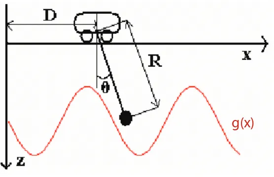
Figure 1.1: The Trolley Control System.
Mathematically, we can describe this dynamic system by x′′(t) = −T(t) sinθ(t)
z′′(t) = −T(t) cosθ(t) D′′(t) = a
1(t)
R′′(t) = a2(t)
x(t) = R(t) sinθ(t) +D(t) z(t) = R(t) cosθ(t)
where (x, z) are the coordinates of the load, the mass of the load is assumed to be 1, the mass of the rope is assumed to be negligible and θ is the angle between the rope and the vertical axis. T is the tension of the rope. D and R are the position of the trolley and the length of the rope, respectively, and a1, a2 are the respective
accelerations of the trolley and the rope.
trolley and acceleration of the rope, through the gas pedal and the crank, for example. Then a1 and a2 are the controlsof the system.
Suppose that in finite time τ we wanted to get the trolley as close as possible to the end of the track (point (1,0)) while keeping the swinging load above the terrain described by function g(x) but no less than 2 meters away from the trolley. Mathematically, this means the addition of two constraints
z(t) ≤ g(x(t)) R(t) ≥ 2 and the objective: minimize (1−D(τ))2.
Common sense tells us that even if we are unaware of strict bounds on the max-imum allowable acceleration, we should ”regularize” the system to disallow infinite acceleration. One way to do this is to modify the objective function, putting small weights on the accelerations of trolley and rope along the entire time interval. Thus the new objective is
min(1−D(τ))2+δ Z τ
0
a1(t)2+a2(t)2dt
where δ is small and positive.
Theoretical control theory results support this common sense logic, requiring the objective function to be positive definite with respect to all controls (see, for example, Table 3.3-1 in [28].)
1.2
Standard Form and Alternative Formulations
min φ(x(tf)) +
Z tf
t0
L(x, y, t)dt (1.1a)
x′ = f(x, y, t) (1.1b)
0 = g1(x, y, t) (1.1c)
0 ≤ g2(x, y, t) (1.1d)
x(t0) = ζ (1.1e)
0 = ψ(x(tf)) (1.1f)
where x(t) :R→Rm1 are states ordifferential variables, and y(t) :
R→Rm2 are
algebraic variables. The functions φ:Rm1 →R and L:Rm1+m2+1 →R determine
what is alternately called the cost function, the objective function or the perfor-mance index. The differential constraints are determined by f : Rm1+m2+1 → Rm1,
the algebraic equality constraints by g1 : Rm1+m2+1 → Rc1 and the algebraic
in-equality constraintsbyg2 :Rm1+m2+1 →Rc2, and boundary conditions determined
by ζ ∈Rm1, ψ :
Rm1 →c
3.
For a problem designed to model a real-life process, the algebraic variables will include thecontrols, such as the acceleration of the trolley and the crank that winds the rope. They will also include algebraic variables such as the tension in the rope that are not controlled by the trolley driver. But from a mathematical standpoint, a control is any subset ofy that determines the solution completely for a particular set of initial conditions.
Notice that a problem with a cost function of the form (1.1a) can be converted into a problem with the cost functionC(x(tf)), i.e. a problem in the so-called Mayer
form, by letting C =φ+x2 wherex2 is another state defined by
Similarly, a problem in which L, f, g1, g2 depend explicitly on t can be converted
into a problem whose functions depend only onxand yby letting t be another state, x3, defined by
x′3 = 1 x3(0) = 0
So the problem (1.1a) is equivalent to a problem of the form
min C(x(tf)) (1.2a)
x′ = f(x, y) (1.2b)
0 = g1(x, y) (1.2c)
0 ≤ g2(x, y) (1.2d)
x(t0) = ζ (1.2e)
0 = ψ(x(tf)) (1.2f)
Finally, notice that a problem of the form (1.1a) or (1.2) is equivalent to the same problem but with t0 = 0 and tf = 1, simply by letting ¯t = t/(tf −t0). The results
presented in the main chapters of this work were proved for problems in different forms. To make them easier to read and compare, we have rewritten some of them in a different form so that most results now refer to problems of the form 1.2.
1.3
Optimality Conditions
equations that, under certain additional conditions, will uniquely determine a local minimum.
When minimizing a function of one variable with no constraints, a critical point occurs where the derivative of the function is zero. In the presence of constraints, the constraints are adjoined to the cost function with the aid of an adjoint variableto form what is sometimes called the augmented performance index which is then differentiated with respect to all variables. For continuous control problems, the first derivative is replaced by the firstvariationand the resulting equations are called the
Euler-Lagrange Equationsalso known asfirst-order optimality conditionsor first-order necessary conditions (for optimality).
For constrained problems, the derivation of the first-order optimality conditions is complicated (see Section 4.1) but for unconstrained problems of the form (1.2) the augmented performance index has the form
J =C(x(tf)) +νTψ(x(tf)) +
Z tf
t0
λT(f(x, y)−x′)dt
and the first-order optimality conditions take the form
x′ = ∇λH (1.3a)
λ′ = −∇xH (1.3b)
0 = ∇uH (1.3c)
x(t0) = ζ (1.3d)
λ(tf) = ∇xC(x(tf)) +νT∇xψ(x(tf)) (1.3e)
whereH(x, u, λ) =λTf(x, u) is the Hamiltonian. See [28], Section 3.2 for a detailed
derivation.
conditions to consider. When minimizing a function of several variables, we are interested in whether its Jacobian is positive-definite. For optimal control problems, this is replaced with conditions such as coercivity (Definition 2.2) written in terms of the solution to a linearized problem or a Ricatti equation. For more information on necessary and sufficient conditions for optimality for different types of problems, see [11].
Suppose that the problem in (1.3) is actually a problem of the form min φ(x(tf)) +
Z tf
t0
L(x, y, t)dt (1.4a)
x′ = f(x, y, t) (1.4b)
x(t0) = ζ (1.4c)
0 = ψ(x(tf)) (1.4d)
”in disguise”. Then the Hamiltonian takes the form λ2L+λTf and we calculate
λ2(tf) = ∇x2φ(x) +x2 = 1 and λ
′
2 = −∇x2H = 0 giving us λ2(t) = 1 for all t. So
for problems of the form (1.4), the first order optimality conditions can be applied without loss of generality to the Hamiltonian defined by H =L+λTf.
1.4
Methods of Solution
Methods for solving optimal control problems can be divided into two basic categories:
direct and indirect methods.
the optimality conditions are so-called gradient algorithms. An overview of these and some of the other methods discussed here can be found in [31].
Direct methods approximate the original problem by a discrete optimization problem, an approach that is sometimes referred to as”discretize then optimize.”
Some direct methods rely on techniques such as shooting or multiple shooting, where the equations (1.2b) – (1.2f) are solved for a particular control, usually assumed piecewise constant on a grid. Then the control is adjusted with the goal of making the cost smaller, and the whole process is repeated until a tolerance is met. The advantage of these methods is the relatively small size of the discretized problem, their major drawback is their stability. For a quick overview of shooting and multiple shooting methods see [3], Chapter 3.
In contrast, the class of methods we will call direct transcription methods dis-cretize the entire problem on a grid, normally by using a collocation method based on a numerical integrator. For a problem in Mayer form (1.2) this amounts to dis-cretizing the differential equations to obtain algebraic equations in the variablesxi, yi,
which represent the values of the states and the algebraic variables at the grid points ti and, for higher order discretization methods, also variablesχij, yij, which represent
the values of states and algebraic variables at the intermediate points. The algebraic constraints and boundary conditions, evaluated at the gridpoints, provide additional constraints for the discretized problem. The resulting problem is a large, sparse non-linear program (NLP). For an overview of methods for solving large, sparse nonnon-linear programs that arise from optimal control problems, see [3], Chapters 1 and 2.
Direct transcription methods are well suited to problems where the functions f, gi are ”black boxes”, since in these cases the formulation of optimality conditions
of this thesis we will present two classes of problems for which direct transcription outperforms other methods, inequality constrained problems that exhibit complicated behavior near the constraint boundary and certain equality constrained problems with high index constraints. But there is one thing that all numerical methods for solving optimal control problems have in common - the need to numerically integrate the differential equation (1.2b).
1.5
Convergence and Discretizations
The focus of this thesis is on the convergence properties of direct transcription meth-ods. Most results given here evaluate convergence of a direct transcription method by the maximum difference between the optimal solution for the original problem and the optimal solution to the nonlinear program that is the discretization of the original problem for a particular discretization method and a particular grid. The grid can be uniform, with N = 1/h evenly spaced nodes h units apart. It can be non-uniform, with the distances between nodes given byhi, i= 0, ..., N −1. Because
finer grids produce larger problems that take longer to solve, we are interested in the relationship betweenh, the maximum distance between gridpoints, and the error. We say that the error in variable z is orderb if there exist ¯h, c >0 such that
max
k kzk−z
∗(t
k)k ≤chb
for all h <¯h.
very useful on certain problems. For an overview of different types of discretizations used with direct transcription, see [31], Chapter 6.
Many of the discretizations used by practitioners for solving optimal control prob-lems, both directly and indirectly, belong to the class of so-called classical Runge-Kutta methods. Some Runge-Kutta methods, like the trapezoid method, which approximates a function by linear splines, are also collocation methods. For our pur-poses, a Runge-Kutta method is any method characterized by its Butcher array, consisting of parameters a ∈Rs×s and b, σ ∈Rs. A Runge-Kutta method discretizes the differential equations (1.2b) as
xi+1 = xi+hi s
X
j=1
bjf(χij, yij), i= 0, ..., N −1
χij = xi+hi s
X
k=1
ajkf(χik, yik), i= 0, ..., N −1, j = 1, ..., s.
So, for the purpose of direct transcription methods, a nonlinear program based on the problem (1.2) obtained with a Runge-Kutta method characterized by (a, b, σ) has the form
min C(xN) (1.5a)
xi+1 = xi+hi s
X
j=1
bjf(χij, yij), i= 0, ..., N −1 (1.5b)
χij = xi+hi s
X
k=1
ajkf(χik, yik), i= 0, ..., N −1, j = 1, ..., s (1.5c)
0 = g1(xi, yi) (1.5d)
0 ≤ g2(xi, yi) (1.5e)
x0 = ζ (1.5f)
0 = ψ(xN) (1.5g)
Many popular integrators, such as Euler’s Method, Trapezoid Method, Hermite-Simpson or RK4, are Runge-Kutta methods. However, in practice, these methods are often implemented in a form different from (1.5), out of considerations ranging from time and storage to robustness.
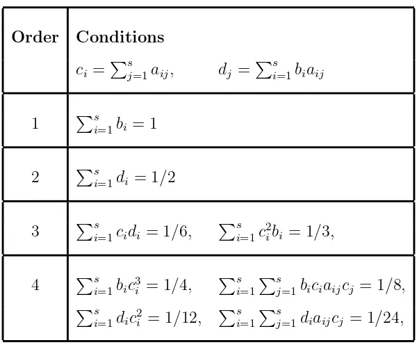
Table 1.1: Order of Runge-Kutta discretization as an integrator.
Order Conditions
ci =Psj=1aij, dj =Psi=1biaij
1 Ps
i=1bi = 1
2 Ps
i=1di = 1/2
3 Ps
i=1cidi = 1/6, Psi=1c2ibi = 1/3,
4 Ps
i=1bic3i = 1/4,
Ps
i=1
Ps
j=1biciaijcj = 1/8,
Ps
i=1dic2i = 1/12,
Ps
i=1
Ps
j=1diaijcj = 1/24,
Runge-Kutta methods are classified as explicit (aij = 0 whenever j ≥ i ) and
necessary.
1.6
Computation
The computational studies presented in this monograph were done using the sparse optimal control code SOCS (see http://www.boeing.com/phantom/socs/) devel-oped at the Boeing company. SOCS is a collection of FORTRAN77 subroutines, suited for solving any optimal control problems with dynamics given by ordinary differential equations, including multiple-phase problems, and problems with right-hand sides of dynamics and constraints described by user-defined functions. For more information on SOCS , see [5].
SOCS allows the user to choose the discretization methods to be used as well as the initial grid. Unless told otherwise, SOCS will formulate the discretization on a coarse grid using a lower order method, find the optimal solution and then use various heuristics to refine the grid and/or switch to a higher order discretization method, reformulate the discretization, and repeat. To demonstrate convergence properties, specifically convergence order, we often ask SOCS instead to solve the problem on a particular grid using a particular discretization method and stop. For more information on mesh refinement and stopping criteria for same, see [3], Section 4.7 For a detailed description of the mesh refinement algorithm currently used in SOCS, see [8] and [7].
(http://www.maplesoft.com) for algebraic manipulations in a number of our the-oretical results as well as to solve optimal control problems using a number of dis-cretizations not implemented in SOCS. All these codes are available in electronic form
Chapter 2
Unconstrained Problems
2.1
Overview
In this chapter we will cover problems of the form
minC(x(tf)) (2.1a)
x′ = f(x, y) (2.1b)
x(t0) = ζ. (2.1c)
Many results relating to convergence of direct transcription methods for optimal control problems belong to Hager, Dontchev and Veliov [12, 13, 14, 15, 16, 19, 20, 21]. We follow their lead in making the following two assumptions about the problem (2.1).
Definition 2.1. The problem (2.1) is said to satisfy the smoothness con-dition if it has a local solution (x∗, u∗) which lies in W2,∞×W1,∞, where Wk,p is
the Sobolev space consisting of vector-valued measurable functions y : [t0, tf] → Rm1
whose jth derivative y(j) lies in Lp for all j = 0, ..., k with the norm
||y||Wk,p =
k
X
Moreover, there exists an open set Ω⊂Rm1 ×
Rm2 and ρ >0 such that
Bρ(x∗(t), u∗(t))⊂Ω
for every t∈[t0, tf], the first two derivatives of f are Lipschitz continuous in Ω, and
the first two derivatives of C are Lipschitz continuous in Bρ(x∗(tf)).
Under the smoothness condition (Definition 2.1), we know that there exists a λ∗ such that x∗, u∗, λ∗ satisfy the optimality conditions (1.3) with ψ = 0.
Let
A(t) =∇xf(x∗(t), y∗(t)), B(t) =∇yf(x∗(t), y∗(t)), (2.3a)
V =∇2xxC(x∗(tf)), Q1(t) =∇2xxH(x∗(t), y∗(t), λ∗(t)), (2.3b)
Q2(t) =∇2xxH(x∗(t), y∗(t), λ∗(t)), Q3(t) =∇2xxH(x∗(t), y∗(t), λ∗(t)). (2.3c)
Definition 2.2. We say that the problem (2.1) satisfies the coercivity con-dition if for any (x, y)satisfying
x′ = A(t)x+B(t)y x(t0) = 0
there exists α >0 such that
x(tf)TV x(tf) +
Z tf
t0
x(t)TQ1x(t) + 2x(t)TQ3y(t) +y(t)TQ2y(t)dt≥α
Z tf
t0
y(t)2dt.
Coercivity is related to positivity of the Hessian of H which makes it a type of 2nd order optimality condition.
D1 ajk= 0 for k ≥j
D2 ρj =Psk=1ajk for j = 1, ..., s D3 bj >0 forj = 1, ..., s
D4 bj =bs−j+1 for j = 1, ..., s
D5 apj
as−j+1,s−p+1 =
bj
bp for j = 1, ..., s−1;p=j + 1, ..., s.
The assumption (D1) means that the RK is explicit by definition and (D5) imposes no additional restrictions on a and b if s < 3. If s = 3 or 4, (D5) imposes only the restriction aj1
as,s−j+1 =
b1
bj for j = 2, ..., s−1.
Hager’s result can be interpreted as follows:
Theorem 2.3. If the optimal control problem (2.1) satisfies smoothness (Defi-nition 2.1) and coercivity (Defi(Defi-nition 2.2) and its RK discretization is at least 2nd
order as an integrator (Table 1.1) and satisfies conditions D.1-D.5 and has a local
optimal solution (x, y), then
max
k kxk−x
∗(t
k)k+ max
k kyk1−y
∗(t
k)k ≤ch2.
See Section 2.4.1 for a proof of how Theorem 2.3 follows from the result in [19]. Note that this result proves only second order convergence, even for methods of higher order.
Runge-Kutta methods that satisfy the conditions X
i∈Nl
bici =
X
i∈Nl
biσi (2.4a)
s
X
i=1
X
j∈Nl
biaij =
X
i∈Nl
bi(1−σi) (2.4b)
X
i∈Nl
bi > 0 (2.4c)
for all l ∈[1, s] where Ni ={j ∈[1, s] :σj =σi}.
The result, reproduced here as Theorem 2.4, is also applicable to problems with generalized control constraints of the form y∈U.
Theorem 2.4. (Adapted from [14]) If the optimal control problem (2.1) satisfies the smoothness and coercivity conditions (Definitions 2.1 and 2.2), and the
Runge-Kutta scheme is 2nd order (see Table 1.1) and satisfies the conditions (2.4), then
for all sufficiently smallh= maxhk, the discretization of (2.1) obtained according to
this Runge-Kutta scheme has a strict local minimizer(x, y)and an associated adjoint variable λ such that, if dydt∗ has bounded variation,
max
i=1,...,N,j=1,...,s||xi−x
∗(t
i)||+||λi−λ∗(ti)||+||yi−1,j−y∗(ti−1,j)|| ≤ch2
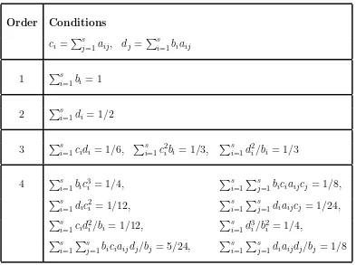
Table 2.1: Order of Runge-Kutta discretization for optimal control.
Order Conditions
ci =Psj=1aij, dj =Psi=1biaij
1 Ps
i=1bi = 1
2 Ps
i=1di = 1/2
3 Ps
i=1cidi = 1/6, Psi=1ci2bi = 1/3, Psi=1d2i/bi = 1/3
4 Ps
i=1bic3i = 1/4,
Ps
i=1
Ps
j=1biciaijcj = 1/8,
Ps
i=1dic2i = 1/12,
Ps
i=1
Ps
j=1diaijcj = 1/24,
Ps
i=1cid2i/bi = 1/12, Psi=1d3i/b2i = 1/4,
Ps
i=1
Ps
j=1biciaijdj/bj = 5/24,
Ps
i=1
Ps
j=1diaijdj/bj = 1/8
in [9], Bonnans and Laurent-Varin developed an algorithm that allowed them to de-rive ”order for optimal control” conditions for orders up to 7. Hager’s theorem can be stated in the following way:
Theorem 2.5. (Adapted from [21], Theorem 2.1) If the optimal control problem (2.1) satisfies the smoothness and coercivity conditions (Definitions 2.1 and 2.2), and
the Runge-Kutta scheme is of order κ for optimal control (Table 2.1) with bi > 0
for each i, then for all sufficiently small h = maxhk, the discretization of (2.1)
an associated adjoint variable λ such that, if dydt∗ has bounded variation,
max
k=0,...,N||xk−x
∗(t
k)|| ≤ chκ
max
k=1,...,N||y(xk, λk)−y
∗(t
k)|| ≤ chκ
max
k=1,...,N||λk−λ
∗(t
k)|| ≤ chκ
where y(xk, λk) is a local minimizer of H corresponding to λ=λk, x=xk.
Theorem 2.5 is the only theoretical result we have come across that proves higher order convergence for a large class of Runge-Kutta methods which includes the meth-ods implemented in many software packages including SOCS, such as the Trapezoid Method, which has the Butcher array representation
a= 0 0 1/2 1/2 , b=
1/2 1/2 , σ= 0 1
and the Hermite-Simpson Method, which can be represented by
a=
0 0 0
5/24 1/3 −1/24 1/6 2/3 1/6
, b= 1/6 2/3 1/6 , σ = 0 1/2 1 .
According to Table 2.1, this makes Trapezoid Method order 2 for optimal control and Hermite-Simpson method order 4.
However, notice that Theorem 2.5 only proves high order convergence of states and multipliers. Control convergence is notoriously harder to prove.
Theorem 2.5 provides a way of post-calculating the controls using the states and multipliers and guarantees that the resulting values are accurate to the same order. This post-calculation procedure would not be hard to implement in SOCS. All one would have to do is use an existing code that implements an unconstrained minimiza-tion algorithm such as some variaminimiza-tion of Newton’s method to find y that minimizes the function H = λT
kf(xk, y) and repeat for every k. For problems of reasonable
size that satisfy Hager’s smoothness and coercivity assumptions this should be both simple and fast.
However, if we tried to do it, we would encounter a big problem: the multiplier estimates produced by SOCS are not as accurate as the discrete multipliers in The-orem 2.5. In the next section, we will demonstrate that this is due to the fact that the theorem assumes a Butcher array implementation whereas SOCS implements more compact variations of popular Runge-Kutta methods such as Trapezoid and Hermite-Simpson. These implementations are mathematically equivalent, so the states and algebraic variables that solve the discretization are the same regardless of implementation, but the multipliers are in fact different.
In particular, for the Trapezoid method (TR) , we will show that, for uniform grids, the compressed implementation used in SOCS produces multipliers that are 2nd order accurate at midpoints, not gridpoints. We will also show that simple interpolation is sufficient to obtain 2nd order estimates of the multipliers at gridpoints. Finally, we will show that the control produced by the TR discretization regardless of implementation is 2nd order accurate at the inside gridpoints, that is, all gridpoints except t0 and tN = tf. This is the first result to show 2nd order convergence in
2.2
Multiplier Convergence
2.2.1
New Theoretical Result
As noted above, TR is a Runge-Kutta method characterized by
α=
0 0
1/2 1/2 , b=
1/2 1/2
, σ=
0 1
.
This means that the TR discretization of problem (2.1) has the form
minC(xN) (2.5a)
xk+1 = xk+
h
2(f(xk, yk1, tk1) +f(χk, yk2, tk2)), k = 0, ..., N −1 (2.5b) χk1 = xk+
h
2(f(xk, yk1, tk1) +f(χk1, yk2, tk2)), k= 0, ..., N −1 (2.5c)
x0 = ζ, (2.5d)
and if the original problem satisfies the assumptions of Theorem 2.5 then (2.5) has a solutionw= (x, u, λ) which satisfies
max
k=0,...,Nkxk−x
∗(t
k)k ≤ ch2
max
k=1,...,Nkλk−λ
∗(t
k)k ≤ ch2.
However, by subtracting equation (2.5c) from (2.5b) we get that χk=xk+1. Also,
since σ = [0,1], tk2 =tk+1 in (2.5b) and therefore yk2 = yk1+1, so that in practice TR
is often simplified and implemented in the compressed form as
minC(xN) (2.6a)
−xk+1+xk+
h
x0 =ζ (2.6c)
whereηk is a small tolerance. Theηkis there because the discretization is imposed as
a constraint and thereby holds only up to a certain tolerance which is above machine precision.
It is clear that when ηk = 0 the two formulations are mathematically equivalent
and therefore they must produce the same optimal values of xk, yk. However, if we
formulate the optimality conditions for (2.5) and (2.6), we can see that the optimal multiplier variables are not related in any obvious ways and, in fact, take on different numerical values. To simplify the notation we set t0 = 0, tf = 1, in what follows.
Theorem 2.6. If the smoothness and coercivity conditions (Definitions 2.1 and 2.2) are satisfied and dydt∗ is of bounded variation and the problem (2.1) is discretized
on a uniform grid h=hi = 1/N, then for all sufficiently small h its compressed TR
discretization (2.6) has a local optimal solution (x, y, λ) that satisfies
max
k=0,...,Nkxk−x
∗(t
k)k ≤ ch2 (2.7a)
max
k=1,...,Nkλk−λ
∗(t
k)k ≤ ch (2.7b)
max
k=1,...,Nkλk−λ
∗
tk−
h 2
k ≤ ch2 (2.7c)
max
k=1,...,N−1
λk+1+λk
2 −λ
∗(t k) ≤ ch 2 (2.7d) max
k=1,...,N−1kyk−y
∗(t
k)k ≤ ch2. (2.7e)
in SOCS.
We have also shown that TR (regardless of implementation) gives second order estimates of the control on the inside gridpoints. Until now, second or higher order convergence in the control was only known to occur with certain restrictive classes of methods (Theorems 2.3 and 2.4), of which neither TR nor any other of the commonly used discretizations implemented in SOCS is a member.
The numerical results in the next section illustrate Theorem 2.6 on a particular example.
2.2.2
Numerical Example
Example 2.1. Consider the example problem from [21]:
min Z 1
0
y(t)2+x(t)y(t) + 5 4x(t)
2dt (2.8a)
x′(t) = 0.5x(t) +y(t) (2.8b)
x(0) = 1. (2.8c)
Note that this problem satisfies the coercivity condition (Definition 2.2) since the quadratic form inside the integral in (2.8a) is positive definite and the problem has one optimal solution given by
x∗(t) = cosh(1−t)
cosh(1) (2.9a)
y∗(t) = −(tanh(1−t) + 0.5) cosh(1−t)
cosh(1) (2.9b)
λ∗(t) = 2 cosh(1−t) tanh(1−t)
cosh(1) . (2.9c)
problem analytically. In Table 2.2, we give the logarithm (base 2) of the max norm of the error in x, y, λfor N = 10,20,40,80. As the number of gridpoints doubles, the logarithm of the error decreases by 2, so the error itself is a quarter of the previous grid error. Thus both x and λ errors are order 2 as proved by Hager.
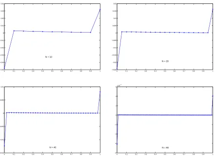
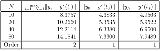
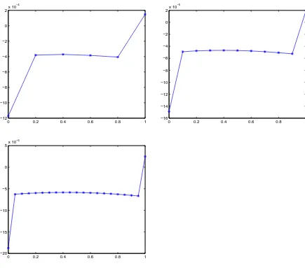
However, when we solve the same problem using SOCS on the same uniform grids (by overriding the grid refinement algorithm and telling SOCS to only use TR), we see in Table 2.3 that even though the resultingxvalues are the same, theλvalues are only first degree accurate just as equation (2.7b) of Theorem 2.6 states. In Table 2.4, we show that, as per equation (2.7c), these values are a second order approximation to the adjoint variables at the midpoints. We also show that, in accordance with equation (2.7d), simple linear interpolation is sufficient to obtain second order approximations to the adjoints on the inside gridpoints. Finally, in Table 2.5, we demonstrate that the controls produced by TR are second order accurate on the inside gridpoints, as stated in equation (2.7e). Figure 2.1 further illustrates this point by graphingy∗−y for N = 10,20,40,80.
In contrast, using SOCS with the discretization specified to be the classical 4th order Runge-Kutta method, given by
α=
0 0 0 0
0 1/2 0 0
0 0 1/2 0
0 0 0 1
, b= 1/6 1/3 1/3 1/6 , σ= 0 1/2 1/2 1
we obtain results that conform exactly to Theorem 2.5. The state and the multiplier λ1 are fourth order approximations to the states and adjoints at the gridpoint, u is
third order, but u post-calculated from x and λ1 in the way given in Theorem 2.5 is
0 0.1 0.2 0.3 0.4 0.5 0.6 0.7 0.8 0.9 1 −0.05
−0.04 −0.03 −0.02 −0.01 0 0.01 0.02 0.03 0.04
N = 10
0 0.1 0.2 0.3 0.4 0.5 0.6 0.7 0.8 0.9 1
−0.025 −0.02 −0.015 −0.01 −0.005 0 0.005 0.01 0.015 0.02
N = 20
0 0.1 0.2 0.3 0.4 0.5 0.6 0.7 0.8 0.9 1
−0.015 −0.01 −0.005 0 0.005 0.01
N = 40
0 0.1 0.2 0.3 0.4 0.5 0.6 0.7 0.8 0.9 1
−8 −6 −4 −2 0 2 4 6x 10
−3
N = 80
Table 2.2: −log2 of uncompressed TR error to gridpoint values ofx, y, λ.
N max
i=0...Nkxi−x∗(ti)k i=1max...Nkλ1i −λ∗(ti)k
10 8.8010 9.4278
20 10.7249 11.1800
40 12.6850 13.0671
80 14.6646 15.0129
Order 2 2
N max
i=0...Nkyi1−y∗(ti)k i=1max...Nky(λ1i, xi)−y∗(ti)k
10 4.3833 9.0806
20 5.3535 10.9346
40 6.3380 13.8634
80 7.3300 14.8282
Order 1 2
Table 2.3: −log2 of compressed TR error to gridpoint values of x, y, λ. N max
i=0...Nkxi−x∗(ti)k i=0max...Nkyi−y∗(ti)k i=1max...Nkλi−λ∗(ti)k
10 8.8010 4.3833 3.3677
20 10.7249 5.3535 4.3446
40 12.6850 6.3380 5.3332
80 14.6646 7.3300 6.3275
Order 2 1 1
Table 2.4: −log2 of compressed TR error in λ: at gridpoint, at midpoint, interpo-lated at gridpoint.
N max
i=1...Nkλi−λ∗(ti)k i=1max...Nkλi−λ∗ ti− h2
k max
i=1...N−1k
λi+λi+1
2 −λ
∗(t
i)k
10 3.3677 8.7633 8.0477
20 4.3446 10.6731 9.9185
40 5.3332 12.6283 11.8554
80 6.3275 14.6053 13.8243
Table 2.5: −log2 of compressed TR error in y: inside gridpoints and endpoints. N max
i=1...N−1kyi−y∗(ti)k ky0−y∗(t0)k kyN −y∗(tf)k
10 8.3757 4.3833 4.9563
20 10.2660 5.3535 5.9522
40 12.2114 6.3380 6.9500
80 14.1841 7.3300 7.9489
Order 2 1 1
Table 2.6: −log2 of RK4 error to gridpoint values of x, y, λ. N i=0max...Nkxi−x∗(ti)k i=1max...Nkλ1i −λ∗(ti)k
5 15.6440 15.8353
10 19.4282 19.7289
20 23.3203 23.6685
Order 4 4
N i=0max...Nkyi1−y∗(ti)k i=1max...Nky(λ1i, xi)−y∗(ti)k
5 9.7356 17.5819
10 12.7113 21.2261
20 15.7039 24.4543
Order 3 3-4
0 0.2 0.4 0.6 0.8 1 −12
−10 −8 −6 −4 −2 0 2x 10
−4
0 0.2 0.4 0.6 0.8 1
−16 −14 −12 −10 −8 −6 −4 −2 0 2x 10
−5
0 0.2 0.4 0.6 0.8 1
−20 −15 −10 −5 0 5x 10
−6
2.3
Open Questions
We have proved some practical results regarding multiplier and control convergence for Trapezoid Method. However, commercial direct transcription codes also use com-pressed versions of other discretizations that may be preferable to TR because they give higher order convergence in the states. The default option in SOCS , for example, is to discretize the problem on a coarse grid using TR, then after two mesh refinement iterations switch to a discretization called Hermite-Simpson method (HS).
Both TR and HS are collocation methods, but whereas the TR approximation to the right-hand side of a differential equation is piecewise linear, HS approximates a function with cubic splines. TR is 2nd order as integrator as well as 2nd order for optimal control, which means that, in its uncompressed form, it gives 2nd order convergence in states, multipliers and post-calculated controls. HS is 4th order as an integrator as well as 4th order for optimal control.
The Butcher-array formulation of HS is given by
xk+1 = xk+h(
1
6f(xk, yk1, tk) + 2
3f(χk1, yk2, tk+12) +
1
6f(χk2, yk3, tk+1)) (2.10) χk1 = xk+h(
5
24f(xk, yk1, tk) + 1
3f(χk1, yk2, tk+12)−
1
24f(χk2, yk3, tk+1))(2.11) χk2 = xk+h(
1
6f(xk, yk1, tk) + 2
3f(χk1, yk2, tk+12) +
1
6f(χk2, yk3, tk+1)). (2.12)
Two implementations of HS are available in SOCS. The default is HS-Compressed. The other one is called HS-Separated. HS-Separated is obtained from the Butcher array formulation by subtracting (2.12) from (2.10) to obtainχk2 =xk+1, then solving
(2.10) forf(χk1, yk2, tk+1
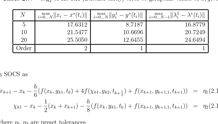
Table 2.7: −log2 of HS-RK (Butcher array) error to gridpoint values of x, y, λ. N max
i=0...Nkxi −x∗(ti)k i=0max...Nkyi1−y∗(ti)k i=0max...N−1kλ1i −λ∗(ti)k
5 17.6312 8.7187 16.8779
10 21.5477 10.6696 20.7249
20 25.5050 12.6455 24.6494
Order 2 1 1
in SOCS as xk+1−xk−
h
6(f(xk, yk1, tk) + 4f(χk1, yk2, tk+12) +f(xk+1, yk+1,1, tk+1)) = η1(2.13)
χk1−xk−
1
2(xk+xk+1)− h
8(f(xk, yk1, tk) +f(xk+1, yk+1,1, tk+1)) = η2(2.14) where η1, η2 are preset tolerances.
The most compact formulation, HS-Compressed, is obtained by solving (2.14) (η2 = 0) forχk1 and consists of only one equation
xk+1−xk−
h
6(f(xk, yk1, tk) + 4f(χ, yk2, tk+21) +f(xk+1, yk+1,1, tk+1)) = η(2.15)
where χis defined exactly by χ=xk+
1
2(xk+xk+1) + h
8(f(xk, yk1, tk) +f(xk+1, yk+1,1, tk+1)).
Note that HS-Compressed has only N(m1+ 2m2) variables andNm1 constraints
compared toN(m1+m2) and Nm1 constraints for TR-Compressed but it offers 4th
degree approximation of the state instead of only 2nd degree. It does not, however, offer a 4th order approximation of adjoints at the gridpoint in the same way that the Butcher array formulation (N(3m1 + 2m2) variables, 3Nm1 constraints) does
according to Theorem 2.5.
0 0.2 0.4 0.6 0.8 1 −2.5
−2 −1.5 −1 −0.5
0x 10
−3
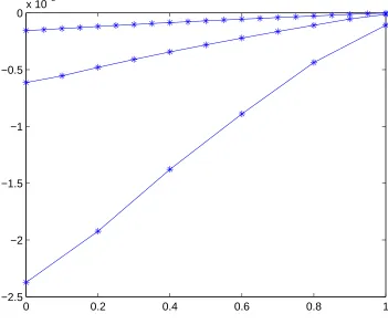
Figure 2.3: Example problem solved with HS. Graph of y∗−y for N = 5,10,20.
Table 2.8: −log2 of HS-Compressed error to gridpoint values of x, y, λ. N max
i=0...Nkxi−x∗(ti)k i=0max...Nky1i −y∗(ti)k i=1max...Nkλi−λ∗(ti)k
5 17.6312 8.7187 2.4610
10 21.5459 10.6696 3.3934
20 25.4973 12.6455 4.3581
Table 2.9: −log2 of HS-Compressed error in λ: at gridpoint, at midpoint, interpo-lated at gridpoint.
N max
i=1...Nkλi−λ∗(ti)k i=1max...Nkλi−λ∗ ti− h2
k max
i=1...N−1k
λi+λi+1
2 −λ
∗(t
i)k
5 2.4610 8.8156 7.0228
10 3.3934 10.7175 8.8161
20 4.3581 12.6697 10.7177
Order 1 2 2
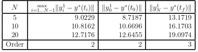
Table 2.10: −log2 of HS-Compressed error in y: inside gridpoints and endpoints. N max
i=1...N−1kyi1−y∗(ti)k ky01−y∗(t0)k ky1N −y∗(tf)k
5 9.0229 8.7187 13.1719
10 10.8162 10.6696 16.1703
20 12.7176 12.6455 19.0974
Order 2 2 3
order respectively (see Table 2.7). However, solving the same example with SOCS demonstrated (see Tables 2.8 – 2.10) that HS-Compressed can only offer a 2nd degree approximation to the adjoints at the midpoint, same as TR.
Unlike with TR, the control error on the inside gridpoints is not significantly smaller than at the ends (Table 2.10, Figure 2.3). However, we did notice the linear nature of the gridpoint errors in Figure 2.3. Notice in Table 2.10 that the endpoint error appears to be 3rd order. Taken together with Figure 2.3, this may indicate that HS-Compressed in fact gives a third order approximation to the control on some rescaled grid. As expected, the uncompressed formulation, which we implemented with Maple, gives multipliers that are 4th order accurate.
the state errors themselves are on the order of 10−6,10−7,10−8 for N = 5,10,20
respectively, whereas the control errors are only on the order of 10−3 to 10−4.
In summary, future work would include
• A theorem similar to Theorem 2.6 for HS-Compressed. We would like to establish 2nd order convergence at the midpoint, and the validity of simple interpolation to obtain 2nd order approximations at the gridpoint. Can adjoint approximations of order greater than 2 be obtained on the original grid or on some other grid, either directly from the discrete multipliers or though some kind of manipulation?
• Some insight into control error with HS. Can we prove 2nd order conver-gence overall for yk1 and perhaps higher order convergence on a subgrid
or a shifted grid as we did with TR? Does yk2 converge to the either the
gridpoint or the midpoint values of the control and to which order? • Studying the differences and similarities between HS-Compressed and
Separated. Are the multipliers produced by Separated and HS-Compressed always the same? What are the advantages of one formula-tion versus the other?
2.4
Proofs
2.4.1
Proof of Theorem 2.3
The paper [19], page 458 makes the following assumptions about a problem of the form (2.1):
A1 There exist an optimal control y∗ and a corresponding trajectory x∗
A2 The differential equation x′ =f(x, y) can be integrated for all y in some neigh-borhood of y∗
A3 There exists an optimal solution χh, yh to the discretization A4 Both the discrete and the continuous optimality conditions hold
A5 The discretization is order b as an integrator, where b ≥2.
A6 If x1, x2 are solutions to x′ = f(x, y) satisfying x1(s) = p1, x2(s) = p2 for some
s∈[0,1] then for allt ∈[0,1],kx1(t)−x2(t)k=O(kp1−p2k).
Now (A1), (A2), (A4) follow from smoothness and (A6) follows from smoothness and coercivity (see [16]), whereas (A3) and (A5) are part of the theorem statement.
The RK discretization of (2.1) has the form
min C(xN) (2.16a)
xi+1 = xi+hi s
X
j=1
bjf(χij, yij), i= 0, ..., N −1 (2.16b)
χij = xi+hi s
X
k=1
ajkf(χik, yik), i= 0, ..., N −1, j = 1, ..., s (2.16c)
Let αjp = aj+1,p+1 for j = 1, ..., s− 1;p = 0, ..., s−2 and αsp = bp+1 for p =
0, ..., s−1. Using (D1), we can rewrite (2.16) as min C(¯xN0)
¯
xij = ¯xi0+hi j−1
X
p=0
αjpf(¯xik,y¯ik), i= 0, ..., N −1, j = 1, ..., s
¯
xi+1,0 = ¯xi,s, i= 0, ..., N −1
¯
x00 = (0,0, ζ)
where ¯xi0 = xi for i = 0, ..., N, ¯xij = χi,j+1 for j = 1, ..., s− 1, ¯yij = yi,j+1 for
j = 0, ..., s−1.
Moreover, we can establish that the following conditions are satisfied
P1 ([19],p.458) ¯xij,y¯ij approximate the state and the control at timeti+ρjhi where
0 =ρ0 ≤...≤ρs = 1. This follows from 0≤σ1 ≤...≤ σs ≤ 1, (D2), (D4) and
the relationship between (¯xij,y¯ij) andxi, χij, yij.
P2 ([19],p.460)αsj 6= 0 for j = 0, ..., s−1, which follows from (D3).
P3 ([19], Eq.39) αsj =αs,s−j−1 for j = 0, ..., s−1, which follows from (D5).
P4 ([19], Eq.38)αpjαsp =αsjαs−j−1,s−p−1 forj = 0, ..., s−2;p=j+1, ..., s−1, which
follows from D.6.
The assumption in [19], Theorem 3.1 that h ∇2
yyH
−1
is bounded in y and h follows directly from coercivity [21]. So the bound on the error in y follows from Lemma 3.1 and Theorem 3.1 in [19] and the bound on the error inx follows from the discretization being 2nd order as an integrator.
2.4.2
Proof of Theorem 2.6
Lemma 2.1. ([21], Proposition 5.1) Let X be a Banach space and let Y be a linear normed space with the norms in both spaces denoted k · k. Let F :X → 2Y be
a set-valued map, let L:X →Y be a bounded linear operator, and let T :X→ Y be continuously Freche´t differentiable in Br(w∗) for some w∗ ∈ X and r > 0. Suppose
that the following conditions hold for some δ∈Y and scalars ǫ, γ, and τ > 0: Q1 T(w∗) +δ ∈F(w∗).
Q2 k ▽T(w)−Lk ≤ǫ for all w∈Br(w∗).
Q3 The map (F − L)−1 is single-valued and Lipschitz continuous in B
τ(π), π =
(T −L)(w∗), with Lipschitz constant γ.
If ǫγ <1, ǫr≤τ,kδk ≤(1−γǫ)r/γ, then there exists a unique w ∈Br(w∗) such that
T(w)∈F(w). Moreover, we have the estimate
kw−w∗k ≤ γ
1−γǫkδk.
Formulate the Hamiltonian for (2.6)
¯
H(x, y, λ) = C(xN) + N−1
X
k=0
λk+1
−xk+1+xk+
h
2(f(xk, yk) +f(xk+1, yk+1))
,
and let
T(w) =
T1(w)
T2(w)
T3(w)
= ¯
Hλk, k = 1, ..., N
¯
Hxk, k = 1, ..., N
¯
Hyk, k = 0, ..., N
where w= (x, y, λ) = (x0, ..., xN, y0, ..., yN, λ1, ..., λN).
We apply function space norms to x, y and λ by considering them as piecewise constant functions on [t0, tf] with respect to the gridpointstk with value xk (yk, λk)
Define a norm on the domain of T by kwk=kxkL∞+kyk
L2 +kλkL∞ (2.17)
and a norm on the range of T by
k(p, q, r)k=kpkL1+kqkL1 +krkL2. (2.18)
Let Ak, Bk, Qik denote A, B, Qi evaluated at t=tk and let L(w) be given by
−xk+1+xk+
h
2(Akxk+Bkyk+Ak+1xk+1+Bk+1yk+1), k= 0, ..., N −1(2.19a) h(Q1kxk+Q3kyk) +
I +h
2A
T k
λk+1−
I −h
2A
T k
λk, k= 1, ..., N −1(2.19b)
h
2(2V xN +Q1NxN +Q3NyN)−
I− h
2A
T N
λN (2.19c)
h
2 Q20y0+Q
T
30x0+B
T
0λ1
(2.19d) h
Q2kyk+Q
T
3kxk+
1 2B
T
k(λk+1+λk)
, k= 1, ..., N −1(2.19e) h
2 Q2NyN +Q
T
3NxN +B
T NλN
. (2.19f)
We will apply Lemma 2.1 (case F = 0) to two different values of w∗,wˆ and ˇw, where
ˆ
x = ˇx = (x(t0)∗, ..., x(tN)∗),
ˆ
λ = (λ∗(t1), ..., λ∗(tf)),
ˇ λ =
λ∗
t0+
h 2
, ..., λ∗
tN−1+
h 2
.
and ˆy,yˇare defined in Lemma 2.5.
Finally, we tie it all together in the proof of Theorem 2.6. The next Lemma is known but we include its proof to illustrate the role of h in the norms used.
Lemma 2.2. Given N ≥1, h= N1, then for any vector z ∈Rm(N+1),
kzkL1 ≤c1kzkL2 ≤c2kzkL∞.
Proof. Let h·,·idenote the Euclidean inner product and let ¯1 be a vector ofN+ 1 ones. Using the Schwartz inequality,
kzkL1 =
N+1
X
i=1
hkzik=h
√
h¯1,√hkziki ≤
√
hk¯1k2k
√ hzk2
= r
N + 1
N kzkL2 ≤ r
2N
N kzkL2 = √
2kzkL2.
For the second inequality,
kzkL2 =
v u u t N+1 X i=1
hkzik2 ≤
v u u t N+1 X i=1 h(max
i kzik)
2 =
r N + 1
N (maxi kzik)
2 ≤√2kzk
L∞.
Lemma 2.3. For all sufficiently small h, the solution xto the system of equations
xk+1 = xk+
h
2(Akxk+Ak+1xk+1) +zk, k = 0, ..., N −1 (2.20a)
x0 = ζ, (2.20b)
where z, ζ are given, can be described by x=M1(z) +M2(ζ)where M1, M2 are linear
Proof. We rewrite (2.20) as ¯Ax=z+e1ζ where the block bidiagonal matrix ¯ A=
I 0 · · · 0
−I− h
2A0 I−
h
2A1 . .. ...
..
. . .. . .. ...
0 0 · · · −I− h
2AN−1 I−
h
2AN
is invertible ande1 = (I,0, ...,0)T. Thus M1 = ¯A−1, M2 = ¯A−1e1.
Lemma 2.4. For all (x, λ)∈Bτ(x∗(tk), λ∗(tk)), whereτ is independent ofh, there
exists a unique y satisfying Hy(x, y, λ) = 0 and ky−y∗(tk)k ≤c(kλ−λ∗(tk)k+kx−
x∗(t
k)k).
Proof. Coercivity implies thatHyy(x∗(t), y∗(t), λ∗(t)) =Q2(t) is invertible for all t
and hence uniformly positive definite since we are working on a closed finite interval [21]. So the result follows from the Implicit Function Theorem.
Lemma 2.5. There exist y,ˆ yˇsatisfying
ky∗(t
k)−yˆkk ≤ ch, k= 0, ..., N
ky∗(tk)−yˇkk ≤ ch2, k = 1, ..., N −1
ky∗(t
k)−yˇkk ≤ ch, k= 0, N
such that y,ˆ yˇsolve H¯yk(x
∗(t
k), y, λ) for λ= ˆλ and λ= ˇλ respectively.
Proof. First, note that
¯ Hyk =
hHy(xk, yk,λk+12+λk), k = 1, ..., N −1 h
2Hy(x0, y0, λ1), k = 0
h
Applying Lemma 2.4 withx=x∗(t
k) andλ=
ˆ
λk+1+ˆλk
2 we obtain, fork= 1, ..., N−
1,
kyˆk−y∗(tk)k ≤ k
λ∗(t
k+1) +λ∗(tk)
2 −λ
∗(t
k)k
= kλ ∗(t
k+1)−λ∗(tk)k
2 ≤ch.
Similarly, if k =N and λ= ˆλN then
kyˆk−y∗(tk)k ≤ kλ∗(tN)−λ∗(tN)k= 0
and if k = 0,
kyˆk−y∗(tk)k ≤ kλ∗(t1)−λ∗(t0)k=ch.
This establishes Lemma 2.5 for ˆy.
For ˇy, we proceed in the same way, noting that, for k= 1, ..., N −1,
λ∗ t
k+h2
+λ∗ t
k− h2
2 −λ
∗(t k)
≤ch2,
but λ ∗
t1−
h 2
−λ∗(t1)
≤ch and λ∗
tN −
h 2
−λ∗(tN)
≤
ch.
Theorem 2.7. In the norms given by equations (2.17) and (2.18), the function
L−1 is Lipschitz continuous everywhere with Lipschitz constant γ = c h.
Proof. Consider the equation L(w)−π = 0 where π =−(p, q, r)∈R3N+1. It can
the quadratic programming problem
min
xk,yk
N−1
X
k=1
Lk(xk, yk) +qkTxk+rkTyk
!
+1
2(hL0(x0, y0) + 2r0y0) +1
2(hLN(xN, yN) + 2hx
T
NV xN + 2qNTxN + 2rTNyN) (2.21a)
xk+1 = xk+
h
2(Akxk+Bkyk+Ak+1xk+1+Bk+1yk+1) +pk (2.21b)
x0 = ζ (2.21c)
where Lk(xk, yk) = 21 xTkQ1kxk+ 2x
T
kQ3kyk+y
T kQ2kyk
. By Lemma 2.3, (2.21) can be written as1
min
y,x
¯
L(x, y) + ¯qTx+ ¯rTy (2.22) x = M1(PBy¯ +p) +M2(ζ) (2.23)
where
P = h 2
I I . .. ... 0 . .. ... 0
... · · · I I , ¯
L = xTQ¯
1x+yTQ¯2y+ 2xTQ¯3y
=
N−1
X
k=1
Lk(xk, yk) +
1
2(L0(x0, y0) +LN(xN, yN) +x
T
NV xN),
¯
q = 1
h(0, q1, ..., qN−1,2qN), ¯
r = 1
h(2r0, r1, ..., rN−1,2rN), ¯
B = (B0, ..., BN).
Substituting (2.23) into (2.22) we obtain the unconstrained problem minyC(y)
where
C(y) = ((yTB¯TPT +pT)M1T +ζTM2T) ¯Q1(M1(PBy¯ +p) +M2(ζ)) +yTQ¯2y
+2((yTB¯TPT +pT)M1T +ζTM2T) ¯Q3y+ ¯qT(M1(PBy¯ +p) +M2(ζ)) + ¯rTy
= yTQy¯ + (φ1+φ2ζ)Ty+φ3(ζ) +φ4
where
¯
Q = B¯TPTM1TQ¯1M1PB¯+ ¯Q2+ 2 ¯BTPTM1TQ¯3
φ1 = 2( ¯BTPTM1TQ¯1 + ¯Q3
T
)M1p+ ¯BTPTM1Tq¯+ ¯r
φ2 = 2 ¯BTPTM1TQ¯1M2+ 2 ¯Q3
T
M2.
Since C(y) = yTQy¯ corresponds to the problem (2.21) with p =q = r = ζ = 0,
the coercivity condition on the original problem impliesyTQy¯ ≥βkyk
L2. So, by [15],
Lemma 4, given y1, y2 corresponding to two different values ¯φ1,φ¯2 of ¯φ = φ
1+φ2ζ,
we have ky1−y2k
L2 ≤ckφ¯1−φ¯2kL2. If ¯φi = ¯φ(pi, qi, ri, ζ), then we have
ky1−y2kL2 ≤ck( ¯BTPTMT
1 Q¯1+ ¯Q3
T
)M1(p1−p2) + ¯BTPTM1T(¯q1−q¯2) + (¯r1−r¯2)kL2.
To make the following discussion more readable, let ¨z =. z1−z2 where z can be
p, q, r, x, y or λ. Note that x=M1p¨is the solution to
xk+1 = xk+
h
2(Akxk+Ak+1xk+1) + ¨pk (2.24a)
Thus we have xk+1 =
I−h
2Ak+1 −1
I+h 2Ak
xk+
I− h
2Ak+1 −1
¨ pk
=
Πki=k−1(I− h 2Ai+1)
−1(I +h
2Ai)
xk−1
+(I− h 2Ak+1)
−1(I+ h
2Ak)(I− h 2Ak)
−1p¨
k−1+ (I−
h 2Ak+1)
−1p¨
k
=
Πki=0(I− h 2A
T
i+1)−1(I+
h 2A T i ) x0 + k X i=0 Πk
j=i(I−
h 2A
T
j+1)−1(I+
h 2A
T j)
(I− h 2Ai+1)
−1p¨
i = k X i=0 Πk
j=i(I−
h 2A
T
j+1)−1(I+
h 2A
T j)
(I− h 2Ai+1)
−1p¨
i.
Let a= maxk=0,...,NkAkk/2 and assume h <1/a, so that, for j = 0, ..., N,
kI+h
2Ajk ≤ 1 +ha k
I− h
2Aj −1
k ≤ (1−ha)−1
We also use the fact that (1 +ha)1/h,(1−ha)−1/h are both bounded from above byea
which in turn is bounded by maxt0<t<tf e
kA(t)k/2. And so we have, fork = 0, ..., N−1,
kxk+1k ≤
k
X
i=0
Πkj=ik(I −
h 2A
T
j+1)−1kkI+
h 2A
T jk
k(I− h 2Ai+1)
−1kkp¨
ik
≤
N−1
X
i=0
(1 +ha)N−i
(1−ha)N−i+1kp¨ik ≤e 2a
N−1
X
i=0
kp¨ik
≤ hckp¨kL1.
Hence
kxkL∞ = max
k kxkk ≤
c hkp¨kL1 and therefore by Lemma 2.2,
kM1p¨kL2 =kxkL2 ≤
The second term can be evaluated as follows: kPTM1T(¯q1−q¯2)kL2 ≤ k
2 hP
TMT
1 (0¨q)kL2 ≤ k
2 hP
T
kL2kMT
1 (0¨q)kL2.
Now
kh2PTkL2 = max
kzkL2=1
q h(z2
1 + (z1 +z2)2+...(zN−1+zN)2+z2N)
= max
kzkL2=1k
(0, z1, ..., zN) + (z1, ..., zN,0)kL2
≤ max kzkL2=1
2k(z0, z1, ..., zN)kL2
= 2. and µ=MT
1 (0q¨) is the solution to
µ0 = µ1+
h 2A
T
0µ1 (2.25a)
µk = µk+1+
h 2A
T
k (µk+µk+1) + ˙qk, k = 1, ..., N −1 (2.25b)
µN =
h 2A
T
where ˙qk = ¨qk for k = 1, ..., N −1, ˙qN = 2¨qN. So we have, for k = 1, ..., N −1,
µk = (I−
h 2A
T
k)−1(I+
h 2A
T
k)µk+1+ (I−
h 2A
T k)−1q˙k
=
Πk+1
i=k(I −
h 2A
T
i )−1(I+
h 2A
T i)
µk+2
+(I− h 2A
T
k)−1(I+
h 2A
T k)(I−
h 2A
T
k+1)−1q˙k+1+ (I −
h 2A
T k)−1q˙k
=
ΠNi=−k1(I− h 2A
T
i )−1(I+
h 2A T i ) µN +
N−1
X
i=k
Πij−=1k(I− h 2A
T
j)−1(I+
h 2A
T j)
(I− h 2A
T i )−1q˙i
=
ΠNi=−k1(I− h 2A
T
i )−1(I+
h 2A
T i )
(I− h 2A
T N)−1q˙N
+
N−1
X
i=k
Πij−=1k(I− h 2A
T
j)−1(I+
h 2A
T j)
(I− h 2A
T i )−1q˙i
=
N
X
i=k
Πij−=1k(I− h 2A
T
j)−1(I+
h 2A
T j)
(I− h 2A
T i)−1q˙i.
Note that the last expression also describes µN.
We calculate an upper bound on kµkk similarly to kxk+1k in (2.24), by letting
a= maxk=1,...,NkATkk/2 and assuming h <1/a, so that, for k = 1, ..., N,
kµkk ≤ N
X
i=k
Πij−=1kk(I−h 2A
T
j)−1kkI+
h 2A
T jk
k(I−h 2A
T
i )−1kkq˙ik
≤
N
X
i=1
(1 +ha)i−1
(1−ha)i kq˙ik ≤
(1 +ha)N
(1−ha)N N
X
i=1
kq˙ik ≤2e2a N
X
i=1
kq¨ik
= c
hkq¨kL1. Also,
kµ0k ≤ k(I +
h 2A
T
0)kkz0k=ckz0k ≤
so that
kµkL∞ = max
k kµkk ≤
c hkq¨kL1. and therefore by Lemma 2.2
kM1Tq¨kL2 =kµkL2 ≤
c hkq¨kL1. Thus we have
ky¨kL2 ≤
c
h(kp¨kL1 +kq¨kL1 +k¨rkL2.) (2.26) Now subtract L(w1)−π2 = 0 from L(w2)−π1 = 0 to obtain
¨
xk+1 = ¨xk+h(Akx¨k+Bky¨k+Ak+1x¨k+1+Bk+1y¨k+1) + ¨pk, (2.27a)
k = 1, ..., N −1 ¨
x0 = 0 (2.27b)
¨
λk = ¨λk+1+
h 2A T k ¨
λk+ ¨λk+1
+h(Q1kx¨k+Q3ky¨k) + ¨qk, (2.28a)
k= 1, ..., N −1 ¨
λN =
h 2A
T Nλ¨N +
h
2(2V xN +Q1Nx¨N +Q3Ny¨N) + ¨qN (2.28b)
Compare (2.24) to (2.27) to conclude kx¨kL∞ ≤
c
hkhB¯y¨+ ¨pkL1 ≤cky¨kL2 + c hkp¨kL1. Next, compare (2.25) to (2.28) to conclude
kλ¨kL∞ ≤ c
N−1
X
k=1
(hkQ1kx¨k+Q3ky¨kk+kq¨kk) +
ch
2 k2Vx¨N +Q1Nx¨N +Q3Ny¨Nk+kq¨Nk
≤ cky¨kL1 +ckx¨kL1 +
c hkq¨kL1 ≤ cky¨kL2 +
c
Combining these results with (2.26), we have kx1−x2kL∞+ky1−y2k
L2+kλ1−λ2kL∞ ≤ c h(kp
1
−p2kL1+kq1−q2kL1+kr1−r2kL2).
This completes the proof of Theorem 2.7.
Theorem 2.8. Given the previous definitions and assumptions it follows in the norm given by (2.18) that,
kT( ˆw∗)k=k(ˆp,q,ˆ r)ˆk = ch2 kT( ˇw∗)k=k(ˇp,q,ˇ r)ˇk = ch3.
Proof. By definition of ˆy,y, we haveˇ krˆkL2 = kˇrkL2 = 0. Using Lemma 2.5 and
the fact that f is Lipschitz continuous we have, for k = 0, ..., N −1, kpˆkk = k −x∗(tk+1) +x∗(tk) +
h 2(f(x
∗(t
k),yˆk) +f(x∗(tk+1),yˆk+1))k
= k −x∗(tk+1) +x∗(tk) +
h 2(f(x
∗(t
k), y∗(tk)) +f(x∗(tk+1), y∗(tk+1))
+h 2(f(x
∗(t
k),yˆk)−f(x∗(tk), y∗(tk))) +
h 2(f(x
∗(t
k+1),yˆk+1)−f(x∗(tk), y∗k+1))k
≤ k −x∗(tk+1) +x∗(tk) +
h 2(f(x
∗(t
k), y∗(tk)) +f(x∗(tk+1), y∗(tk+1)))k
+chkyˆk−y∗(tk) + ˆyk+1−y∗(tk+1)k
≤ c1h3+c2h2 =ch2.
giving kpˆkL1 =ch2.
For ˇp we have, fork = 1, ..., N −2,
kpˇkk ≤c1h3 +chkyˇk−y∗(tk) + ˇyk+1−y∗(tk+1)k=ch3.
But
kpˇ0k ≤ c1h3+chkyˇ0−y∗(t0) + ˇy1−y∗(t1)k
and
kpˇN−1k ≤ c1h3+chkyˇN−1−y∗(tN−1) + ˇyN −y∗(tN)k
≤ c1h3+h(c2h2+c3h) =ch2.
So
kpˇkL1 ≤
N−2
X
k=1
h(c1h3)
!
+ 2h(c2h2)≤ch3.
To evaluate ˆq and ˇq, we first rewrite them in terms of Hx. Thus we have, for
k = 1, ..., N −1, ˆ
qk = λ∗(tk+1)−λ∗(tk) +
h 2fx(x
∗
(tk),yˆk)T(λ∗(tk) +λ∗(tk+1))
= λ∗(tk+1)−λ∗(tk) +hHx
x∗(tk),yˆk,
λ∗(t
k) +λ∗(tk+1)
2
and
ˆ
qN = −λ∗(tN) +
h 2fx(x
∗(t
N),yˆN)Tλ∗(tN) +Cx(x∗(tN))
= h
2Hx(x ∗(t
N),yˆN, λ∗(tN))
and for ˇq we have ˇ
qk = λ∗
tk+
h 2
−λ∗
tk−1+
h 2
+hHx x∗(tk),yˇk,
λ∗ t
k+h2
+λ∗ t
k−1+ h2
2
!
, k = 1, ..., N −1
ˇ
qN = −λ∗
tN −
h 2 + h 2H
x∗(tN),yˇN, λ∗
tN −
h 2
+λ∗(tN).
Next, let ˜H(t, λ) = Hx(x∗(t), y∗(t), λ). Consider the RK method given by α =
[1/2], b = [1], σ = [0]. Checking Table 1 in [21], we determine that it is a 2nd order method. So, integrating λ′ =−H(t, λ) from˜ t
k totk+1 with step size h, we obtain
˜
q1k=−λ∗(tk+1) +λ∗(tk)−hHx
x∗(tk), y∗(tk),
λ∗(t
k) +λ∗(tk+1)
2
Applying the 2nd order RK method given by α = [1/2], b = [1], σ = [1/2] with step size h to the same equation from tk−1+ h2 totk+ h2, we obtain
˜
qk2 = −λ∗
tk+
h 2
+λ∗
tk−1+
h 2
−hHx x∗(tk), y∗(tk),
λ∗ t
k+ h2
+λ∗ t
k−1+ h2
2
!
=O(h3).
We also define
˜
q3 = λ∗
tN −
h 2 − h 2H
x∗(tN), y∗(tN), λ∗
tN −
h 2
+λ∗(tN) =O(h2),
which is obtained by applying the 1st order RK method given byα= [0], b = [1], σ= [1],with step size h/2 to the equation λ′ =−H(t, λ) from˜ t
N − h2 totN.
Finally, we use Lipschitz continuity of Hx and λ∗ and Lemma 2.5 to show
kqˆkk = kqˆk+ ˜qk1k ≤ch3+chkyˆk−y∗(tk)k ≤ch2,
kqˆNk ≤ ch
and
kqˇkk = kqˇk+ ˜qk2k ≤ch3+chkyˇk−y∗(tk)k ≤ch3,
kqˇNk = kqˇN + ˜q3k ≤h3c+chkyˇN −y∗(tN)k ≤ch2.
Thus
kqˆkL1 ≤
N−1
X
k=1
h(c1h2)
!
+h(c2h)≤ch2
and
kqˇkL1 ≤
N−1
X
k=1
h(c1h3)
!
+h(c2h2)≤ch3.