CREATING THE BEST ROUTING BY HEURISTIC ALGORITHM

(1)

Http://www.ijetmr.com©International Journal of Engineering Technologies and Management Research [28]

CREATING THE BEST ROUTING BY HEURISTIC ALGORITHM

Mehmet ŞİRİN *1_{, Tuğba ALTINTAŞ}2_{, Ali GÜNEŞ}3

*1

Department of Computer Engineering, Istanbul Aydin University, Istanbul, Turkey 2

Department of Health Sciences, Uskudar University, Istanbul, Turkey 3

Department of Computer Engineering, Istanbul Aydin University, Istanbul, Turkey

Abstract:

In this study, Travelling Salesman Problem (TSP), an NP-hard problem, is addressed. In order to get the best results with a view to directing TSP heuristics, the ant colony algorithm was used for solution purposes. The purpose was to solve the problem of setting a course for the bread distribution trucks of Istanbul Halk Ekmek (Public Bread) Company using the ant colony algorithm on TSP. A liquid called Pheromone, which ants release in order to establish communication among them, is known as the most fundamental matter to provide this communication. In this research, artificial ants, which function with the logic of finding the shortest path in the area where they are located, were utilized. The purpose of our programme is to determine the shortest route for the arrival of the distribution trucks to the kiosks where bread is sold to the public. The route developed by the programme is displayed over Google maps.

Motivation/Background: Explain the importance of the problem investigated in the paper. Include here a statement of the main research question.

Method: Give a short account of the most important methods used in your investigation. Results: Present the main results reported in the paper.

Conclusions: Briefly present the conclusions and importance of the results. Concisely summarize the study’s implications. Please do not include any citations in the abstract.

Keywords: Ant Colony Algorithm; Travelling Salesman Problem; Web-Based Application; Routing.

Cite This Article: Mehmet ŞİRİN, Tuğba ALTINTAŞ, and Ali GÜNEŞ. (2017). “CREATING

THE BEST ROUTING BY HEURISTIC ALGORITHM.” International Journal of Engineering

Technologies and Management Research, 4(12), 28-42. DOI: 10.29121/ijetmr.v4.i12.2017.132.

1. Introduction

(2)

DOI: 10.5281/zenodo.1134113

the way for the definition of the new problems in the literature and to the development of new techniques for their solution. Travelling Salesman Problem has been one of the important optimisation problems on which researchers have worked in recent years. Travelling Salesman Problem (TSP) is an optimization problem trying to find the way or the tour/route which starts from a certain place and returns to the same point after visiting all the points in the list only once. In terms of the difficulty to be solved, it is classified among NP-Hard Problems [1].

In the literature, vehicle routing problem TSP is expressed as a more improved version. This is so because there are more vehicles used and more constraints applied. In Travelling Salesman Problem,

 The seller wants to sell his goods in "n” number of cities,

 The seller wants to complete the tour in the shortest way and by visiting n number of cities only once,

 As the number of cities increases, the difficulty of the problem increases.

 The aim of the problem is to be able to present the shortest path to the salesman. Simply stated, in a symmetric problem with n cities, the number of possible tours is n!/2. When the problem is asymmetrical, it becomes n!.

The Vehicle Routing Problem was first studied by Dantzig and Ramser in 1959 [2]. In that study, the aim was to minimize the vehicle routing in order to minimize the cost of transporting gasoline to the petrol stations and the distance covered. Below is an illustration of the TSP Problem.

Figure1: Travelling Salesman Problem

2. Basic Routing Problems

(3)

DOI: 10.5281/zenodo.1134113

2.1.Travelling Salesman Problem (TSP)

Travelling Salesman Problem has come into existence as a result of the improvement of the problems with separate start and end points. The return of the vehicle to the start point is necessary for the realization of the tour. This increases the complexity of the situation. The goal is to find the sequence through which the points are passed with a view to minimizing the total time and the distance of the tour. Waste collection and school vehicle routes are among examples of these kinds of routing problems; It is possible to increase the number of the examples. Such problems are generally referred to as "Travelling Salesman Problem" [4].

2.2.Chinese Postman Problem (CPP)

Chinese Postman problem is the solution of the problem with minimal cost, provided that each and every target point must be passed at least once. CPP was first researched in 1962 by a Chinese mathematician, Mei-Ko Kwan. The problem arose with the necessity for a postman to distribute letters he receives from a postal office by visiting all the streets in the city in the shortest possible way. After the distribution of the letters, the postman must return to the point where he begins the tour [5]. Although CPP resembles the Travelling Salesman Problem (TSP), there are significant differences between them. The TSP is a node routing problem and it is about finding the shortest tour possible provided that each node is visited only once (Hamiltonian path). The main difference between CPP and TSP is that in CCP, instead of nodes, it is necessary to pass through the edges connecting these nodes and this must happen at least once [6]. If a Euler path is not achieved in the graph of the CCP problem, it could be possible to pass through edges more than once in order to complete the tour.

2.3.Multiple Travelling Salesmen Problems (MTSPs)

These are the situations where the shortest route is found in traveling salesman problems by adding more than one vehicle. N vehicles leave a warehouse and return to the same place. Each vehicle should visit at least one node. There is no restriction for visiting more than one node.

2.4.Single-Warehouse, Multiple-Vehicle and Multiple-Stop Distribution Problems

This is the most common routing problem. The solution method for this problem is to find the distribution paths that will enable the vehicles leaving from the same warehouse to find the shortest route for all stops/points and to return back to the warehouse. In this problem, demands in all points are found deterministically. Studies were carried out by Golden on this subject [7].

2.5.Multiple-Warehouse, Multiple-Vehicle and Multiple-Stop Distribution Problems

(4)

DOI: 10.5281/zenodo.1134113

2.6.Single Warehouse, Multiple-Vehicle and Estimated Demand Distribution Problems

The difference of this problem compared to TG Problem is that the demand in distribution points is unknown. Since the quantity of the demand is not known, the probability distribution is utilized. For the solution of such types of problems, heuristic solution methods are used.

2.7.Capacity Constrained BRT

BRT uses, all points/stops as warehouses. This problem is a vehicle routing problem where each customer is visited by a single vehicle. The capacities of the trucks which go to the same point, that is a warehouse, should not be exceeded. The purpose is to minimize the total cost.

2.8.Cost Constrained BRT

Its difference from Capacity Restricted Model is that in this model, the restriction of the vehicle cost is taken as the basis rather than vehicle capacity restriction.

2.9.Cost and Capacity Constrained BRT

The methods used for the solution of the Capacity Restricted problem and Cost Restricted problem are also used in this model. However, the model is constructed by the use of both restrictions at the same time.

2.10.Time-Constrained BRT

This is the most difficult version of vehicle routing problem. In this problem, modelling is made with the condition that each customer has to be served within a certain period of time.

3. TSP Application Areas

Some of the areas where TS Problem is used commonly are as following:

 Determining the routes for certain types of vehicles (services, patrol cars, etc),

 The Distribution of the goods by the Seller from one or more than one warehouse to

sales points,

 Routing Problems of the Planes,

 Delivery Problem of the Online Sales,

 Distribution Problems (Newspapers, posts, bread, beverages, etc.),

 Gathering of the warehouse materials.

4. TSP Solution Methods

(5)

DOI: 10.5281/zenodo.1134113

4.1.Precise Solution Methods

Precise Solution Methods find the best solution. But the solution time increases exponentially depending on the size/extent of the problem. It is more appropriate for the solution of small and medium level problems. The solution method is easy and provable. There is no single method finding an appropriate and precise solution to all vehicle routing problems.

4.1.1. Cutting Plane

It is aimed to reach the most appropriate solution with a whole number by getting rid of some parts of the appropriate solution parameters for which cutting plane algorithms are prepared [8]. In other words, it is the generation of the whole number solution by making use of the constraints. If the new solution after addition of the constraints is a whole number, that means best solution is found. If the number which is found is still a fractional number, then the process of solution is continued by adding constraints until a whole number is obtained.

4.1.2. Branch and Bound Algorithm

In 1983, branch and bound algorithm was developed by Balas and Toth. By disregarding the sub-tour constraints, it was transformed into an assignment problem. It aims to find the routes by the method of adding lines and columns. In order to prevent the assignment of unknown routes, penalty coefficient is applied and by solving it from the beginning once again, the best solution is obtained.

4.1.3. Branch and Cut Algorithm

It is made by the combination of branch-bound and cutting plane methods [9] For the solution of the problem, first of all, the model is established by using the objective function and the constraints. The sub-tours used in the solution of the model are equalized to zero and problem is divided into branches. Then, the optimum result is found by adding constraint to the branches that are already obtained [10].

4.1.4. Dynamic Programming

Dynamic Programming divides the problem into sub-problems that are independent from each other. By using the solutions of these sub-problems, appropriate vehicle routes are obtained.

4.2.Classical Heuristic Solution Methods

(6)

DOI: 10.5281/zenodo.1134113

i 4.2.1. Route-Establishing Heuristics

These were developed between 1959 and 1990. Route establishing heuristics start the solution of the problem with assignments that will not be realized. It aims at the best solution by adding an edge between two nodes. While adding edges, it is controlled whether the vehicle capacity is respected or not.

4.2.2. Dantzig and Ramser’s Method

Vehicle Routing Problem was first studied by Danzig and Ramser in 1959. With that study, it was aimed that the vehicle routings were minimized so that the routes are determined in the shortest way and with the lowest cost according to the criteria set by the customers in the gasoline service stations [13]. According to the algorithm used, if the total demand of two points is more than the capacity of the vehicle, these two points should be connected [2].

4.2.3. Clarke and Wright’s Savings Algorithm

It was developed by Clarke and Wright in 1964 by drawing on the study made by Dantzig and Ramser. It is one of the most used algorithms among route-establishing heuristic algorithms. Even if any two points are not connected, the vehicle leaving the warehouse will go and return to and from each point. After the points are connected to each other, first, the vehicle will go to the first point and then to the second point and then will return back to the warehouse. Accordingly, there will be savings depending on the difference between the situation where two points are not connected and the situation where two points are connected. The achievement of the savings is shown in Figure 2.

j j

Figure 2: The achievement of the savings

4.2.4. Nearest Neighbour (NN)

(7)

DOI: 10.5281/zenodo.1134113

Figure 3: Nearest Neighbour Algorithm

4.2.5. Route-Developing Heuristics

Route-developing heuristics take the first established solution as the beginning and develop it further. In each repetition, the route is changed, and it is controlled whether the change is a better solution or not [14] [15].

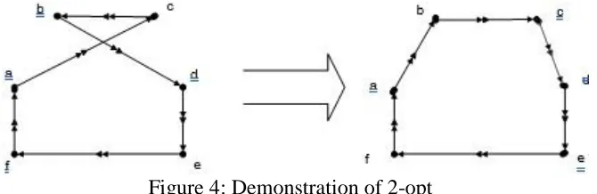
4.2.6. 2-Opt Algorithm

It was first developed by Cores in 1958. While a random solution could be taken as the beginning solution, it is also possible to choose the appropriate solution. With the algorithm, first, pair of points is chosen over the possible solution (a-c, b-d). Then, the places of the two points are changed without skewing the tour (a-b, c-d). The change of the points is shown in figure 4.

Figure 4: Demonstration of 2-opt

If the new found solution is better than the previous one, it is accepted. Otherwise, it continues with the first solution. In this method, the locations of only two points are changed and other points remain fixed. It continues until it is no longer possible to find a better solution with dual change and all possibilities are tried.

4.2.7. 3-Opt Algorithm

(8)

DOI: 10.5281/zenodo.1134113

Figure 5: Demonstration of 2-opt

4.2.8. K-Opt Algorithm

In K-Opt Algorithm, 4 or more points are chosen. Although much more time is spent for a solution in k-opt algorithm, the result obtained shows slight improvement. [15].

4.2.9. Two-Phase Methods

In two-phase methods, points are divided between vehicles without exceeding capacity limits. In the second phase, a route is drawn for each vehicle [14]

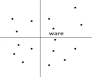
4.2.10.Sweep Algorithm

It is a two-phase algorithm developed by Gillett and Miller in 1971. In the first phase, the warehouse is chosen as the centre and all points are drawn on the coordinate plane as shown in Figure 6. In the second phase, the value of the angle between warehouse and X (East-West) axis, is, is calculated for each i point.

Figure 6: Marking of the points and the warehouse on the coordinate plane.

(9)

DOI: 10.5281/zenodo.1134113

Figure 7: Grouping of the points

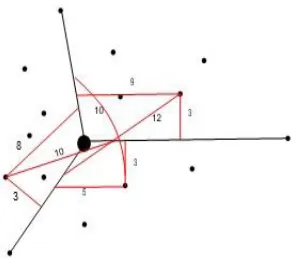
4.2.11.Fisher and Jaikumar Algorithm

It was developed by Fisher and Jaikumar in 1981 as a two-phase method. The number of customers is determined for each vehicle. The customers among which the distance is the biggest are chosen. The distances between the points, the routes developed, and the warehouses are calculated. Considering the capacity limits, the nearest points, routes are assigned as shown in Figure 8. In the second phase TSP is solved [17]

Figure 8: Fisher and Jaikumar Algorithm

4.2.12.Christofides, Mingozzi and Toth

It was developed as a two-phase method by Christofides, Mingozzi and Toth in 1979. This method was developed in order to solve the vehicle routing problems with time, distance and capacity constraints. It produces the result in accordance with the parameters of λ≥1 and µ≥1 given as input by the user. The better one is taken among two solutions. This procedure is repeated for different values of λ and µ parameters. While in the first phase the series are found, in the second phase parallel routes are obtained [18] [19].

4.3.Meta-heuristic Solution Methods

(10)

DOI: 10.5281/zenodo.1134113

precise solution methods. With meta-heuristic methods, the solution of these problems could take much shorter time. For this reason, it is the most practical method for the solution of large-scale and complex problems. Since they could provide the nearest solution to the best one (second best solution) in a short period of time, they are utilized extensively [20] [11] [21].

4.3.1. Taboo Search

It was developed by Glover and Laguna in 1989. Taboo search algorithm makes the achievement of the best result as it enables researches both in positive and negative directions [20] [15]. The exclusion list is the main feature of taboo search. This is continuously updated and hence, prevents the repetition of the algorithm. However, if the solution is the best one found until that time, the even if it is on the exclusion list, the solution is accepted and the solution (process) is continued. In general, the solutions first get worse and then start getting better.

As taboo search could find the second best solution in a very short time period, it is one of the most used methods [20].

4.3.2. Genetic Algorithm

Generic algorithm is the imitation of the naturally developed processes in the problem solution. Problem-solving paradigm was proposed for the first time by Holland in 1975.

First of all, it is started with a solution obtained with other heuristic methods. This is called beginning population. Each parameter of the solution is described as a gene, and the whole solution is accepted as a chromosome. After the completion of the first chromosomes, new chromosomes are created by crossing of the two existing chromosomes or by mutation of a chromosome. With the changing of chromosomes, small changes are made in the values of the genes. In this way, it is aimed to decrease the local minimums. All chromosomes are passed through suitability function and the chromosomes which are most distant from their functions are found and eliminated. The best chromosome, that is the best solution, is obtained.

4.3.3. Simulated Annealing

It was developed by Kirkpatrick et al. in 1983. The purpose of the method is to decrease the possibility of choosing the negative progress instead of positive, through repetition. In this way, while at the beginning there are leaps in the positive section the value of possibility approaches to zero as the second best solution is approached and hence the solution area is narrowed [20].

4.3.4. Ant Colony

(11)

DOI: 10.5281/zenodo.1134113

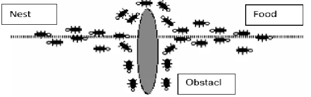
Figure 9: The path followed by ants from their nest to the food

The path followed by the ants before which an obstacle is placed is shown in Figure 10.

Figure 10: The ants facing an obstacle

While the ants not facing an obstacle could follow a single path in order to reach to the food. Once an obstacle placed in their path, not they are faced with two alternative roads. The possibility of choosing each of these paths is equal. This choice is randomly made by the ants.

Figure 11: The choice of ants for the path after having faced an obstacle

Ants leave a chemical door called pheromone. Other ants could decide the path to follow, which path is long, and which one is shorter with the help of the odor of this liquid. They choose the paths to follow to reach to the food according to the density of this odor. In this way, after a while, depending on the density of that odor, the usage of the longer path is diminished. In this way, the shortest way is found by the ant [20] [15]. This ants’ behaviour is seen in Figure 12.

(12)

DOI: 10.5281/zenodo.1134113

Although ant colony algorithm is developed in order to solve Travelling Salesman Problem, in the studies made in recent years, it has also been used in situations where more than one vehicle is added and in the solutions of vehicle touring problems by additional constraints [20].

4.3.5. Artificial Bee Colony

It is an algorithm developed by Karaboğa in 2005, by making use of the way the bees search for food in nature. The algorithm is composed of bees with a duty (employed bees) and bees without a duty; foods and positive & negative feedback. The employed worker bees transmit the information related to the place and the quality of the food they bring from certain resources, to other bees. The bees without a duty yare classified into two groups: onlooker bees and scout bees and they search for new sources of food. Scout bees make up to 5-10% of all bees existing in the hive [20].

4.3.6. Particle Swarm Optimization

It was developed by Kennedy and Eberhart by making use of the behaviours of bird swarms. While searching for food, birds are in interaction with each other and they follow the nearest bird. These interactions are determined as the possible particles of the solution and by following the best particle at that movement they try to find the solution. It is easy to use/apply as there are limited number of parameters in the algorithm [22].

5. Application

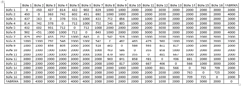
For the sample TSP problem, routing of the vehicles belonging to İstanbul Halk Ekmek Company (Public Bread Inc) was studied. The kiosks where the bread was sold were divided into 3 groups according to 3 factories owned by Halk Ekmek Company. and the routes were created on the basis of these factories. The vehicle route was studied for the Cebeci District which was covered by Cebeci factory. The distances between the kiosks existing in the route and their distances to the factory were determined. Each vehicle in the factory has a capacity of 246 cases of bread. The problem was solved with ant colony algorithm. The distances of the kiosks located in Cebeci Region are exhibited in Table 1 below.

(13)

DOI: 10.5281/zenodo.1134113

5.1.The Solution with TSP Ant Colony Algorithm

The parameters used in the ant colony optimization are as following:

α (alpha): It is related to the amount of Pheromone trace to be used for the current problem. It shows the level of the pheromone to be used for tracing.

Β (beta): It is related to the level of hermeneutics to be used in the current problem.

ρ (rho): It shows the evaporation rate of pheromone for the current problem.

m: the number of ants needed for the algorithm used in the Ant Colony Optimization.

Termination condition (Iteration number): It is related to the number of iterations to be applied to the current problem.

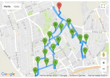
For 16 kiosks existing in our application, the most appropriate parameter values appear as follows: alpha:1; beta; 1; Rho:1; the number of iterations: 250 and the number of ants: 90. When the application is run for Cebeci district, the shortest path is found as shown in Figure 13.

Figure 13: The illustration of the best route for Cebeci District

(14)

DOI: 10.5281/zenodo.1134113

Table 2: Distances on the route. Destination Distance (meter)

FACTORY 2000

Kiosk 12 1000

Kiosk 13 406

Kiosk 14 566

Kiosk 16 709

Kiosk 15 725

Kiosk 9 1000

Kiosk 7 528

Kiosk 6 643

Kiosk 2 451

Kiosk 5 602

Kiosk 1 432

Kiosk 3 437

Kiosk 4 378

Kiosk 8 546

Kiosk 10 463

Kiosk 11 355

Total Distance 11241

As a result of the Ant Colony Algorithm applied for the İstanbul Halk Ekmek factory and 16 Kiosks in Cebeci District, the best route is calculated to be 11,241 meters.

6. Conclusion and Suggestions

In this study, TSP Problems were introduced, and solution methods were discussed. In order to find the best routing of the vehicles, a web-based application was developed and Ant Colony Algorithm (ACA) was used for this application.

As a result of the test carried on during this study, an application enabling the vehicles of the company to save time was developed. By using ACA for 16 kiosks existing in the Cebeci District, in addition to the savings in time, the shortest distribution to the kiosks was maintained with a view to decreasing the costs.

The number of the factories and kiosks used in the study could be further increased. It is applicable to an increased number of points. This study aimed at introducing TSP solution techniques to the academicians making their researches in this area and to provide the manager with a general understanding of the subject.

References

[1] G. Laporte and I. H. Osman, Potvin, J., Y., (1996). “Genetic algorithms for the travelling salesman problem”, forthcoming in Annals of Operations Research on "Metaheuristics in Combinatorial Optimization",eds. 63: 339-370

(15)

DOI: 10.5281/zenodo.1134113

Http://www.ijetmr.com©International Journal of Engineering Technologies and Management Research [42] [3] Bellman, R. (1958), “On a routing problem”, in Quarterly of Applied Mathematics, 16(1): 87-90. [4] Cruyssen, V. D. P., Rijkaert. M.,(1978), “Heuristic for the asymetric travelling

salesmanproblem”, The Journal of the Operational Research Society, 29(7):697–701.

[5] Ahuja, R. K., Magnanti, T. L., Orlin, J. B. (1993), “Network Flows: Theory, algorithmsand applications”, Prentice Hall: New Jersey, 37:211-276.

[6] Eiselt, H. A.,, Gendreau, M., Laporte, G.(1995), “Arc routing problems, Part 1:TheChinese Postman Problem”, Operations Research, 43(2): 231–242.

[7] Golden, B.,Bodin L., Doyle T., Stewart W,(1980), “Approximate Traveling Salesman Algorithms”,Operations Research, June 1, : 694-711.

[8] Pan, L., (2015). Cutting Plane Method. The Chinese University of Hong Kong,Operations Research and Logistics Jan. 20.

[9] Araque, J.R., Kudva, G., Morin, T.L., Pekny, J.F., (1994). A branch-and-cut algorithm for vehicle routing problems. Annals of Operations Research 50, 37-59.

[10] Başkaya Z., Avcı Öztürk, B.,(2005). Tamsayılı programlamada dal kesme yöntemi ve bir ekmek fabrikasında oluşturulan araç rotalama problemine uygulanması. Uludağ Üniversitesi İktisadi ve İdari Bilimler Fakültesi Dergisi Cilt XXIV, Sayı 1, s. 101-114.

[11] Cordeau, J.F., Gendreau, M., Laporte, G., Potvin, J.Y., Semet, F., (2002). A Guide to Vehicle Routing Heuristics. The Journal of the Operational Research Society, Vol. 53, No. 5 pp. 512-522. [12] Bozyer, Z., Alkan, A., Fığlalı, A., (2014). Kapasite Kısıtlı Araç Rotalama Probleminin Çözümü

için Önce Grupla Sonra Rotala Merkezli Sezgisel Algoritma Önerisi. Bilişim Teknolojileri Dergisi, Cilt: 7, Sayı: 2

[13] Atmaca, E., (2012). Bir Kargo Şirketinde Araç Rotalama Problemi ve Uygulaması. Türk Bilim Araştırma Vakfı Dergisi, Cilt:5, Sayı:2, Sayfa: 12-27

[14] Eryavuz, M., Gencer, C., (2001). Araç Rotalama Problemlerine Ait Bir Uygulama.Süleyman Demirel Üniversitesi İktisadi ve İdari Bilimler Fakültesi C.6, S.1, s.139-155.

[15] Nilsson, C., (2003). Heuristics for the Traveling Salesman Problem. Linköping University. [16] Nurcahyo, G.W., Alias, R.A., Shamsuddın, S.M., Sap., M.N.M., (2002), Sweep Algorithm in

Vehicle Routing Problem For Public Transport. Jurnal Antarabangsa (Teknologi Maklumat) 2(2002): 51-64.

[17] Ropke, S., (2005). Heuristic and exact algorithms for vehicle routing problems.

[18] Düzakın, E., Demircioğlu, M., (2009). Araç Rotalama Problemleri ve Çözüm Yöntemleri. Çukurova Üniversitesi İİBF Dergisi Cilt:13. Sayı:1, ss.68-87.

[19] Laporte, G., (1992). The Vehicle Routing Problem: An overview of exact and approximate algorithms. European Journal of Operational Research 59, 345-358.

[20] Şahin, Y., Eroğlu, A., (2014). Kapasite Kısıtlı Araç Rotalama Problemi İçin Metasezgisel Yöntemler: Bilimsel Yazın Taraması.Süleyman Demirel Üniversitesi İktisadi ve İdari Bilimler Fakültesi Dergisi C.19, S.4, s.337-355.

[21] Genreau, M., Potvin, J.Y., Braysy, O., Hasle, G., Lokketangen, A., (2007). Metaheuristics for the vehicle routing problem and its extensions: a categorized bibliography. CIRRELT-2007-27.

[22] Çevik, K.K., Koçer, H.E., (2013). Parçacık Sürü Optimizasyonu ile Yapay Sinir Ağları Eğitimine

Dayalı Bir Esnek Hesaplama Uygulaması. Süleyman Demirel Üniversitesi Fen Bilimleri Enstitüsü Dergisi, 17 (2), 39-45.

*Corresponding author.