https://doi.org/10.5194/wes-3-819-2018
© Author(s) 2018. This work is distributed under the Creative Commons Attribution 4.0 License.
Analysis of control-oriented wake modeling tools
using lidar field results
Jennifer Annoni1, Paul Fleming1, Andrew Scholbrock1, Jason Roadman1, Scott Dana1, Christiane Adcock1, Fernando Porte-Agel2, Steffen Raach3, Florian Haizmann3, and David Schlipf3
1National Wind Technology Center, National Renewable Energy Laboratory, Golden, CO, 80401, USA 2Ecole Polytechnique Federale de Lausanne (EPFL), Wind Engineering and Renewable Energy Laboratory
(WIRE), EPFL-ENAC-IIE-WIRE, 1015 Lausanne, Switzerland
3Stuttgart Wind Energy (SWE), University of Stuttgart, Allmandring 5B, 70569 Stuttgart, Germany
Correspondence:Jennifer Annoni ([email protected])
Received: 25 January 2018 – Discussion started: 8 February 2018
Revised: 11 September 2018 – Accepted: 29 September 2018 – Published: 1 November 2018
Abstract. The objective of this paper is to compare field data from a scanning lidar mounted on a turbine to control-oriented wind turbine wake models. The measurements were taken from the turbine nacelle looking downstream at the turbine wake. This field campaign was used to validate control-oriented tools used for wind plant control and optimization. The National Wind Technology Center in Golden, CO, conducted a demon-stration of wake steering on a utility-scale turbine. In this campaign, the turbine was operated at various yaw misalignment set points, while a lidar mounted on the nacelle scanned five downstream distances. Primarily, this paper examines measurements taken at 2.35 diameters downstream of the turbine. The lidar measurements were combined with turbine data and measurements of the inflow made by a highly instrumented meteorological mast on-site. This paper presents a quantitative analysis of the lidar data compared to the control-oriented wake mod-els used under different atmospheric conditions and turbine operation. These results show that good agreement is obtained between the lidar data and the models under these different conditions.
1 Introduction
Wind plant control can be used to maximize the power pro-duction of a wind plant, reduce structural loads to increase the lifetime of turbines in a wind plant, and better integrate wind energy into the energy market (Johnson and Thomas, 2009; Boersma et al., 2017). Typically, wind turbines in a wind plant operate individually to maximize their own per-formance regardless of the impact of aerodynamic interac-tions on neighboring turbines. There is the potential to in-crease power and reduce overall structural loads by prop-erly coordinating turbine control actions. Two common wind plant control strategies in the literature include wake steer-ing and axial induction control. There has been a signifi-cant amount work done on wake steering, showing that this method has the most potential to increase power production (Annoni et al., 2015; Gebraad et al., 2016). Wake steering typically uses the yaw misalignment of the turbines to
redi-rect the wake around downstream turbines. Various compu-tational fluid dynamics simulations and wind tunnel experi-ments have shown that this method can increase power with-out substantially increasing turbine loads (Gebraad et al., 2016; Fleming et al., 2014; Jiménez et al., 2010). Yaw-based wake steering control has also been used in optimization studies of turbine layouts to improve the annual energy pro-duction of a wind plant (Fleming et al., 2016; Thomas et al., 2015; Stanley et al., 2017). Recent computational fluid dy-namics (CFD) studies have determined that the shape of the wake and atmospheric stability are significant factors in wake steering (Vollmer et al., 2016).
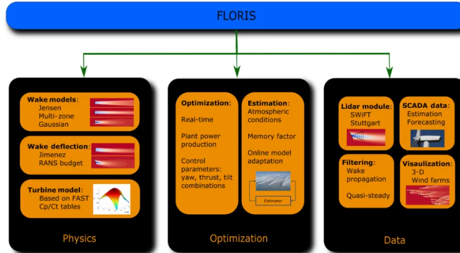
op-Figure 1.The FLORIS tool set is comprised of three main sections: (1) physics, (2) optimization, and (3) data.
timization with feedback to adjust to changing conditions in the atmosphere or wind farm, e.g., turbine down for main-tenance. Lastly, control-oriented models are also useful for large-scale analysis and assessing the impact of controls and optimization on annual energy production. Overall, these models are critical to the success of wind farm controllers and, as a result, full-scale validation of these control-oriented models is essential and a high priority in this area of research. A full-scale demonstration of wake steering is necessary to understand the benefits of wake steering and to validate the benefits predicted by simulations. Wind tunnel tests have been conducted that show encouraging results that match simulation results based on wake redirection (Campagnolo et al., 2016; Schottler et al., 2016). In addition, there are pre-liminary results of the benefits of wake steering from an off-shore commercial wind plant (Fleming et al., 2017b). The National Wind Technology Center also conducted a detailed full-scale demonstration in which a utility-scale turbine op-erated at various yaw offsets while the wake was measured using a scanning lidar. In this paper, the lidar data collected from this campaign are used to validate control-oriented tools that are used for wind plant control. The main contributions of this work include a review of control-oriented models used for wake steering as well as a quantitative analysis of these models with respect to full-scale lidar results. The results between the wake models and lidar data show good agree-ment under various atmospheric and turbine operating con-ditions, as shown in Sect. 4. This is an encouraging result that provides confidence in previously reported benefits of wake steering. The wind plant control tools, including wake
mod-els, turbine modmod-els, and lidar modmod-els, used in wind plant con-trols are introduced in Sect. 2. The field campaign is briefly introduced in Sect. 3. Finally, Sect. 5 provides conclusions and discusses future work.
2 Modeling
FLORIS is defined as a set of control and optimization tools used for wind farm control developed at the National Re-newable Energy Laboratory and TU Delft; see Fig. 1. This tool models the turbine interactions in a wind plant and can be used to perform real-time optimizations to improve wind plant performance and integrate SCADA data collected at wind plants. This section focuses on the wake models, tur-bine models, and the lidar module used in this paper.
2.1 Wake model
2.1.1 Jensen model
The Jensen model has been used for numerous studies on wind plant controls (Jensen, 1983; Johnson et al., 2006; Katic et al., 1986). This model has a low computational cost due to its simplicity and is based on assumptions that there is a steady inflow, linear wake expansion, and the velocity in the wake is uniform at a cross section downstream. The turbine is modeled as an actuator disk with uniform axial loading in a steady uniform flow.
Consider the example of a turbine operating in free-stream velocity,U∞. The diameter of the turbine rotor plane is
de-noted byDand the turbine is assumed to be operating at an induction factor,a. A cylindrical coordinate system is placed at the rotor hub of the first turbine with the streamwise and radial distances denoted byxandr, respectively. The veloc-ity profile at a location (x, r) is computed as
u(x, r, a)=U∞(1−δu(x, r, a)), (1)
where the velocity deficit,δu, is given by
δu=
2aD+2Dkx 2
, if r≤D+2kx
2 .
0, otherwise.
(2)
In this model, the velocity,u, is defined in the axial (x) di-rection and the remaining velocity components are neglected. The wake is parameterized by a tuneable nondimensional wake decay constant,k. Typical values ofkrange from 0.01 to 0.5 depending on ambient turbulence, topographical ef-fects, and turbine operation. For example, if the ambient tur-bulence is high, then the wakes within the wind farm will recover faster due to the mixing of the wake. As a result, the kvalue will be higher, indicating that the wake will recover faster. There is no standard rule for howkvaries with turbu-lence intensity.
Limitations
The Park model can be used to compute the power produc-tion and velocity deficit of a turbine array. This is useful in determining the operating conditions of a wind farm to maxi-mize power. However, it has no notion of added turbulence in the downstream wake due to varying turbine operation. The assumptions are based on a steady inflow acting on an actua-tor disk with uniform axial loading and as noted in Frandsen et al. (2006); the Jensen model does not conserve momen-tum. Despite its limitations, the Jensen model can be com-puted in fractions of a second and can provide some insight into turbine interaction that can be used to understand the results obtained from higher-fidelity models. In addition, if uncertainty is included, the Jensen model performs well and predicts wake interactions well under normal operating con-ditions.
2.1.2 Multi-zone
The multi-zone model, developed in Gebraad and Van Wingerden (2014), is a modification of the Jensen model described in the previous section. Modifications were made to better model the wake velocity profile and effects of partial wake overlap, especially in yawed conditions. The multi-zone model defines three wake zones,q: (1) near-wake zone, (2) far-wake zone, and (3) mixing-wake zone. The effective velocity at the downstream turbinei is found by combining the effects of each of the wake zones of the upstream turbinej:
ui=U∞
1−2
v u u u t X j
ajσq3=1cj,q
Ximin
Aoverlapj,i,q
Ai ,1 2 , (3)
whereXiis thexlocation of turbinei,Aoverlapj,i,q is the overlap
area of a wake zone,qof a turbineiwith the rotor of turbine j, andci,q(x) is a coefficient that defines the recovery of a
zoneqto the free-stream conditions.
ci,q(x)=
D
i
Di+2kemU,q(γi)[x−Xi]
2
, (4)
wheremU,qis defined as
mU,q(γi)=
MU,q
cos(aU+bUγi)
(5)
forq=1,2,3 corresponding to the three wake overlap zones, whereaU andbU represents tuned model parameters,Di is
the rotor diameter of turbinei,γi is the yaw offset of
tur-binei, andMU,q are tuned scaling factors that ensure that
the velocity in the outer zones of the wake will recover to the free-stream conditions faster than the inner zone. The param-eters of the model were tuned to match the results from high-fidelity wake simulations (Gebraad et al., 2016). The most influential parameter iskebecause it defines both wake
ex-pansion and wake recovery. Additional details can be found in Gebraad et al. (2016).
Limitations
2.1.3 Gaussian model
Lastly, a Gaussian model is incorporated in the overall FLORIS wake modeling and control tools. This model was introduced by several recent papers including Abkar and Porté-Agel (2015), Bastankhah and Porté-Agel (2014, 2016), Niayifar and Porté-Agel (2015), and Dilip and Porté-Agel (2017). This model includes a Gaussian wake to describe the velocity deficit, added turbulence based on turbine operation, and atmospheric stability.
Velocity deficit
The velocity deficit of a wake is computed by assuming a Gaussian wake, which is based on self-similarity theory of-ten used in free shear flows, (Pope, 2000). An analytical ex-pression for the three-dimensional velocity deficit behind a turbine in the far wake can be derived from the simplified Navier–Stokes equations as
u(x, y, z) U∞
=1−Ce−(y−δ)2/2σy2e−(z−zh)2/2σz2 (6)
C=1−
s
1−(σy0σz0)M0
σyσz
M0=C0(2−C0) C0=1−
p 1−CT,
whereC is the velocity deficit at the wake center, δ is the wake deflection (see Sect. 2.2), zh is the hub height of the
turbine,σydefines the wake width in they direction, andσz
defines the wake width in thezdirection. Each of these pa-rameters are defined with respect to turbinei; subscripts are excluded for brevity. The subscript “0” refers to the initial values at the start of the far wake, which is dependent on am-bient turbulence intensity,I0, and the thrust coefficient,CT.
For additional details on near-wake calculations, the reader is referred to Bastankhah and Porté-Agel (2016). Abkar and Porté-Agel (2015) demonstrate thatσyandσzgrow at
differ-ent rates based on lateral wake meandering (ydirection) and vertical wake meandering (zdirection). The velocity distri-butionsσzandσyare defined as
σz
d =kz
(x−x0)
d +
σz0
d , where σz0
d =
1 2
r u
R
u∞+u0 , (7)
σy
d =ky
(x−x0)
d +
σy0
d , where σy0
d =
σz0
d cosγ , (8)
whereky defines the wake expansion in the lateral direction
andkz defines the wake expansion in the vertical direction.
For this study, ky andkz are set to be equal and the wake
expands at the same rate in the lateral and vertical directions. The wakes are combined using the traditional sum of squares method (Katic et al., 1986), although alternate methods are proposed in Niayifar and Porté-Agel (2015).
Atmospheric stability
This model also accounts for physical atmospheric quanti-ties such as shear, veer, and changes in turbulence inten-sity (Abkar and Porté-Agel, 2015; Niayifar and Porté-Agel, 2015). Shear, veer, and turbulence intensity measurements are typically available in field measurements and will be used to characterize atmospheric stability in this particular model. It should be noted that these three parameters do not suffi-ciently characterize atmospheric stability as defined in Stull (2012). Other parameters such as vertical flux and tempera-ture profiles are necessary to fully captempera-ture atmospheric sta-bility.
This model is a three-dimensional wake model that in-cludes shear by using the power log law of wind:
Uinit U∞ = z zhub αs , (9)
whereαs is the shear coefficient andUinit indicates the
ini-tial flow field. A high shear coefficient, αs>0.2, is
typi-cally used for stable conditions and a low shear coefficient, αs<0.2, is typically used for unstable conditions (Stull,
2012).
This wake model also takes into account veer associated with wind direction change across the rotor. A rotation factor is added to the Gaussian wake (Eq. 6) such that
u(x, y, z) Uinit
=1−Ce−(a(y−δ)2−2b(y−δ)(z−zhub)+c(z−zhub)2)
a=cos
2φ
2σ2
y
+sin
2φ
2σ2
z
b= −sin 2φ
4σ2
y
+sin 2φ
4σ2
z
c=sin
2φ
2σ2
y
+cos
2φ
2σ2
z
, (10)
whereφ is the amount of veer across the rotor when this equation represents a standard Gaussian rotation.
Lastly, turbulence intensity is accounted for in the model by linking ambient turbulence intensity to wake expansion. An empirical relationship is provided in Niayifar and Porté-Agel (2015):
ky=0.38371I+0.003678, (11)
whereI represents the turbulence intensity, andkaandkbare
tuning parameters whereka=0.38371 andkb=0.003678 in
Niayifar and Porté-Agel (2015). As stated previously,kyand
kzwill be set equal in this study.
Added turbulence
example, if a turbine is operating at a higher thrust, this will cause the wake to recover faster. Conversely, if a turbine is operating at a lower thrust, this will cause the wake to re-cover slower. Conventional linear flow models have a single wake expansion parameter that does not change under var-ious turbine operating conditions. Niayifar and Porté-Agel (2015) provided a model that incorporated added turbulence due to turbine operation:
I = v u u t N X j=0
(Ij+)2+I2
0, (12)
where N is the number of turbines influencing the down-stream turbines, I0 is the ambient turbulence intensity, and
the added turbulence due to turbinei,Ii+, is computed as
I+=Aoverlap
0.8ai0.73I00.35(x/Di)−0.32
, (13)
whereI0is the ambient turbulence intensity andais the
ax-ial induction factor of the turbine, which can be defined in terms ofCTbased on Burton et al. (2001) and Bastankhah
and Porté-Agel (2016):
a≈ 1
2 cosγ
1−p1−CTcosγ
.
In Niayifar and Porté-Agel (2015), the number of turbines, N, used to determine the added turbulence isN=1. In this formulation,N is determined based on a predefined distance to the downstream turbine rather than only including the in-fluence of one turbine. For example, this model considers contributions to the added turbulence intensity from turbines within 15D. This has been shown to be beneficial, especially with closely spaced turbines. Studies have shown that the added turbulence intensity has reached an equilibrium point between two and three turbines downstream (Chamorro and Porté-Agel, 2011).
Limitations
This wake model is an analytical model with approximations made from the steady-state Navier–Stokes equations based on free shear flows. In addition, unlike the previous two mod-els, this model conserves momentum. However, it relies on a linear wake expansion model and has six tuning parame-ters based on empirical relationships for wake expansion and turbulence intensity (Eqs. 11 and 13). The main benefits of this model come from the ties to physical measurements in the field such as shear, veer, and turbulence intensity and its roots in free shear flow theory.
2.2 Wake deflection
The wake models defined above include wake deflection models that approximate the amount of lateral movement
based on the yaw misalignment of the turbine. Two wake de-flection models are defined in the FLORIS wind plant mod-eling and control framework and are briefly described in this section.
2.2.1 Jimenez model
An empirical formulation was presented in Jiménez et al. (2010) and used in the multi-zone formulation (Gebraad et al., 2016). When a turbine is yawed, it exerts a force on the flow that causes the wake to deflect and deform in a par-ticular direction. The angle at the wake centerline is defined as
ξ(x)≈ ξ
2 init
1+2kdDx ξinit(a, γ)=
1 2cos
2γsinγ C
T, (14)
whereξinitis the initial skew angle from the wake centerline
andkdis a tuneable deflection parameter. In Gebraad et al.
(2016), the wake deflection angle is integrated to determine the amount of deflection,δ, achieved by yaw misalignment in the spanwise (y) direction:
δ(x)=
x
Z
0
tanξ(x)dx (15)
δ(x)≈
ξinit
152kdx
D +1
4
+ξinit2
30kd D
2kdx
D +1
5
−ξinitD 15+ξ
2 init
30kd .
The deflection,δ, is achieved by integrating a second-order Taylor series approximation as shown in Gebraad et al. (2016).
2.2.2 Bastankhah model
In Bastankhah and Porté-Agel (2016), wake deflection due to the yaw misalignment of turbines is defined by performing a budget analysis on the Reynolds-averaged Navier–Stokes equations. The wake deflection angle at the rotor is defined by
θ≈ 0.3γ
cosγ
1−p1−CTcosγ
, (16)
and the initial wake deflection,δ0, is defined as
δ0=x0tanθ, (17)
wherex0is the length of the near wake as defined in
wake due to wake steering is defined as
δ=δ0+ θ E0
5.2 r σ
y0σz0 kykzM0
ln
(1.6+ √
M0)
1.6qσσyσz
y0σz0−
√
M0
(1.6−√M0)
1.6q σyσz
σy0σz0+
√
M0
, (18)
whereE0=C02−3e1/12C0+3e1/3. Expressions for the other
symbols in the above equation are provided in Sect. 2.1.3. See Bastankhah and Porté-Agel (2016) for details on the derivation.
2.2.3 Wake asymmetry
Wake deflection is known to be asymmetric based on the sign of the yaw misalignment. In particular, positive yaw angles are more effective than negative yaw angles (Fleming et al., 2018). Previously, it was speculated that there was a rotation-induced lateral offset that is caused by the interaction of the wake rotation with the shear layer (Gebraad et al., 2016). An empirical correction used to account for asymmetry is pre-sented in Gebraad et al. (2016).
Fleming et al. (2018) propose that there is an asymmetry in the wake that can be described by counter-rotating vortices, turbine rotation, and shear rather than actual deflection. Up-dates to the FLORIS wake modeling framework to reflect the asymmetry will be done in future work.
2.3 Turbine model
In addition to wake modeling tools, a turbine model is used in the wind plant tools to provide a realistic description of turbine interactions in a wind plant. The turbine model con-sists of a CP/CT table based on wind speed and constant
blade pitch angle generated by FAST (Jonkman, 2010). The coupling betweenCPandCTis critical in understanding the
benefits of wind plant controls.CP andCTcan also be
cou-pled using actuator disk theory, which is based on the turbine operation defined by an axial induction factor,a:
CP=4a(1−a)2 (19)
CT=4a(1−a).
It is important to note thatCP andCT values are used that
correspond to the local conditions each turbine is operating in. For example, a turbine operating in a wake has a different CP/CTthan a turbine operating in free-stream conditions.
The steady-state power of each turbine under yaw mis-alignment conditions is given by Gebraad et al. (2016):
P =1
2ρACPcosγ
pu3, (20)
wherepis a tuneable parameter that matches the power loss due to yaw misalignment seen in simulations. In actuator disk
theory (Burton et al., 2001),p=3. However, based on large-eddy simulations, the turbine power in yaw misalignment has been shown to match the output whenp=1.88 for the NREL 5 MW. Field observations run fromp=1.4 (Fleming et al., 2017b) top=2.2.
2.4 Lidar model
Finally, in this work a lidar model has been added to the FLORIS wind plant tools. This lidar model is based on the scanning lidar at the University of Stuttgart used in this study. This allows for direct comparison between lidar data col-lected by the scanning lidar and the wake model used. In particular, the scanning lidar used in the field campaign takes a weighted average of nine points along the line-of-sight tra-jectory. A lidar model is necessary to ensure this direct com-parison. If any of the nine points are outside of the wake, the weighted average may lead to a more conservative estimate of the flow in the wake. More details on the lidar used in the wake steering campaign can be found in Raach et al. (2016, 2017) and Fleming et al. (2017a).
The velocity computed by the scanning lidar is based on a line-of-sight velocity. The lidar model used in the FLORIS framework computes the line-of-sight velocity,vLOS, in the
same way that the lidar model computes the line-of-sight ve-locity so that each point scanned by the lidar can be com-pared directly to points computed by the wake model. The li-dar computes a line-of-sight velocity for each point scanned. In particular, one scan point consists of Nweights weighted
points that provide a robust velocity measurement at that lo-cation. In other words,Nweightspoints are used in a weighted
sum to provide a robust velocity measurement at that scan point. The velocity at a single point can be computed as
ui= Nweights
X
j=0
ajeupj, (21)
whereaj represents the weights assigned to each point,i
in-dicates the scan point, andu= [ui, vi, wi]T is the weighted
sum of the measured velocity points eup. Typically the
weights are assigned in a Gaussian manner.
Furthermore, the wind vector u= [ui, vi, wi]T is
pro-jected onto the normalized laser vector point [xi, yi, zi]T
with a focus distance offi=
q
xi,I2 +yi,I2 +z2i,I and the re-sultingvLOS,iis
vlos,i=
xi,I
fi
ui,I+
yi,I
fi
vi,I+
zi,I
fi
wi,I. (22)
Additional details are provided in Raach et al. (2016). This model can be used in conjunction with the field data to per-form closed-loop wind plant controls as is done in Raach et al. (2016). In addition, future work could use the simu-latedvLOS computed using this lidar model to fill gaps that
Figure 2.Lidar scan pattern used at the five locations downstream of the turbine.
Table 1.Test turbine details.
Rated power (kW) 1500
Hub height (m) 80
Nominal rotor diameter (m) 77 Rated wind speed (m s−1) 14
3 Field campaign
A wake steering demonstration was conducted at the Na-tional Wind Technology Center using a utility-scale tur-bine. The utility-scale turbine operated at various yaw mis-alignment conditions and the resulting wake was continually recorded by a nacelle-mounted lidar. The campaign started in September 2016 and concluded in April 2017. This sec-tion describes the turbine, the meteorological tower used to record local conditions, and the lidar system mounted on the nacelle of the turbine. Details were first reported on the lidar field campaign in Fleming et al. (2017a). This paper expands the analysis and provides a quantitative comparison between the control-oriented models presented and the lidar data col-lected in this campaign.
3.1 Setup of the field campaign
The turbine used in this wake steering demonstration was the Department of Energy (DOE) 1.5 MW GE SLE turbine owned by the U.S. DOE and operated by the National Re-newable Energy Laboratory. Details on the turbine are pro-vided in Table 1.
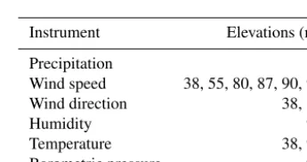
The met tower is located 161 m upstream of the turbine in the predominant wind direction. The met tower was instru-mented in accordance with IEC 61400-12-1. Table 2 lists the instrumentation used on the met tower. The turbine nacelle
Table 2.Meteorological tower instrumentation details.
Instrument Elevations (m)
Precipitation 1
Wind speed 38, 55, 80, 87, 90, 92
Wind direction 38, 87
Humidity 90
Temperature 38, 90
Barometric pressure 90
wind speed and wind direction are measured, recorded, and synchronized with the met tower data.
The lidar data are limited to a region in which the met tower is upstream of the turbine. The hub-height wind speed and wind direction measurements from the met tower are used to described the mean wind speed, wind direction, and turbulence intensity. The wind direction recorded at 38 and 87 m on the met tower is used to compute veer.
3.2 Lidar specifications
The University of Stuttgart scanning lidar system consists of two parts: (1) a WINDCUBE V1 from Leosphere and (2) a scanner unit developed at the University of Stuttgart. A two-degrees-of-freedom mirror is used for redirecting the beam to any position within the physical limitations of the mirror. The lidar can scan an area of 0.75D×0.75D using up to 49 measurement points and five scan distances. The scan rate is dependent on the number of pulses used for each mea-surement position. The lidar system has been used for lidar-assisted control using inflow and wake measurements; see Raach et al. (2016).
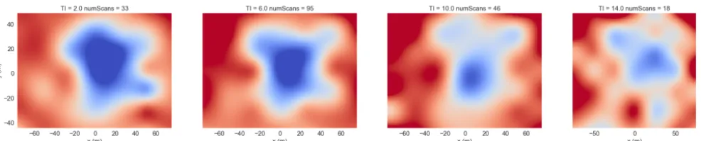
dis-Figure 3.Lidar data at 180.95 m downstream at different turbulence intensities ranging from 2.0 % to 14.0 %. The title of each plot indicates the turbulence intensity and the number of scans used to produce each time-averaged figure.
tances from 1D to 2.8D simultaneously. Each scan consists of 49 points and one scan takes 48 s on average. At each mea-surement point the lidar uses 10 000 laser pulses to measure the line-of-sight wind speed, vLOS, described in Sect. 2.4.
Scans of similar atmospheric conditions and turbine opera-tion are aggregated to produce a mean or median scan.
4 Results
The results presented in this section show the comparison between the wake models described in Sect. 2 and the lidar data collected in the field campaign described Sect. 3. The re-sults focus on comparisons of the velocity deficit behind the turbine, the wake deflection achieved in yaw misalignment conditions, and varying atmospheric conditions.
4.1 Data processing
It is important to note how the lidar data were processed for this study. The lidar data were first processed to filter out im-plausible data. Specifically, several methods were applied to check for hard-target measurements, filter out lidar data with a bad carrier-to-noise ratio, and check for plausibility of the measurement data. The data are also reduced through certain considerations, including (1) periods when the met tower is upstream of the turbine, (2) periods when the turbine is pro-ducing at least 100 kW, and (3) periods when the difference between the target and realized yaw misalignment is small. In particular, the instruments on the met tower that are used to measure wind speed and direction are more reliable when they are not operating in the wake of nearby turbines or in the wake of their own tower due to blockage effects. We also chose to only include data for which the turbine is operat-ing normally. In this case, we define that as producoperat-ing more than 100 kW. The turbine operation affects the wake proper-ties and we need to ensure that we are comparing times when the turbine is performing as expected. Similarly, we only in-clude times when the turbine yaw controller is tracking the specified offset within a few degrees to make a direct com-parison with models.
4.2 Atmospheric conditions
First, the lidar data collected in the field campaign were an-alyzed based on atmospheric conditions. In particular, tur-bulence intensity was examined to understand the behavior of each model under varying turbulence intensity conditions. Figure 3 shows the lidar scans at 180.95 m downstream (ap-proximately 2.5D downstream). The turbulence intensity was computed for each lidar scan and separated into four bins with centers of 2 %, 6 %, 10 %, and 14 % with a wind speed of 8 m s−1. Figure 3 shows that the wake is strongest in low turbulence conditions and dissipates quickly in high turbu-lence conditions. This is consistent with previous work in-vestigating the effects of atmospheric conditions on wakes (Smalikho et al., 2013). It is important to note that each im-age was generated with the maximum number of scans avail-able after processing the data. More scans lead to a more robust measurement of the wake. A statistical analysis is pre-sented in Fig. 4, which indicates the effects of the limited number of scans processed.
Figure 4 shows how the control-oriented engineering mod-els presented in this paper compare with the lidar data. The velocity deficit behind the turbine was computed by averag-ing the velocity across a “virtual” rotor and movaverag-ing this ro-tor across the domain in the spanwise direction (shown in Vollmer et al., 2016). The bands indicate a 95 % confidence interval. A larger band indicates that fewer scans were pro-cessed. Each model was tuned to a subset of the lidar data, which included primarily low turbulence intensity data with a mean turbulence intensity of approximately 5 %. The val-ues of each of the model parameters are shown in the Ap-pendix. It is important to note that these values are tuned for the near wake due to the close proximity of the lidar scans to the turbine (2.35D). Although these measurements are near the turbine, the effects of turbulence intensity can still be ob-served along with wake deflection. Tuning the models appro-priately with training data from this proximity, the models are able to perform reasonably well under varying atmospheric conditions and varying turbine operations even at these close proximities.
Figure 4.Velocity deficit at 180.95 m downstream computed using lidar data, the Gaussian wake model, multi-zone wake model, and the Jensen wake model under different turbulence intensity conditions.
Figure 5.Lidar data at 180.95 m downstream at different yaw misalignments ranging from 0 to 25◦. The title of each plot indicates the yaw angle and the number of scans used to produce each time-averaged figure.
within the confidence interval. This is expected as these mod-els were tuned to low turbulence scenarios. However, when going to high turbulence intensity scenarios, they underpre-dict the velocity deficit significantly. This is because neither the Jensen nor the multi-zone model has turbulence intensity as an input to the model. The Gaussian model, however, is able to capture both low and high turbulence intensity scenar-ios; i.e., the model lies within the confidence interval bands under each turbulence scenario examined. This highlights the fact that, even under varying atmospheric conditions, the Gaussian model is able to accurately capture scenarios that it was not explicitly tuned for. The Jensen and multi-zone mod-els can be retuned to fit high turbulence intensity data as well. Those values are also indicated in the Appendix.
4.3 Wake deflection
Wake deflection was also analyzed using the lidar data from this campaign. Figure 5 shows the wake deflection under tur-bine yaw misalignment observed by the scanning lidar at 180.95 m downstream. Under larger yaw angles, the wake deflects and deforms as has been reported in Howland et al. (2016) and Fleming et al. (2017b).
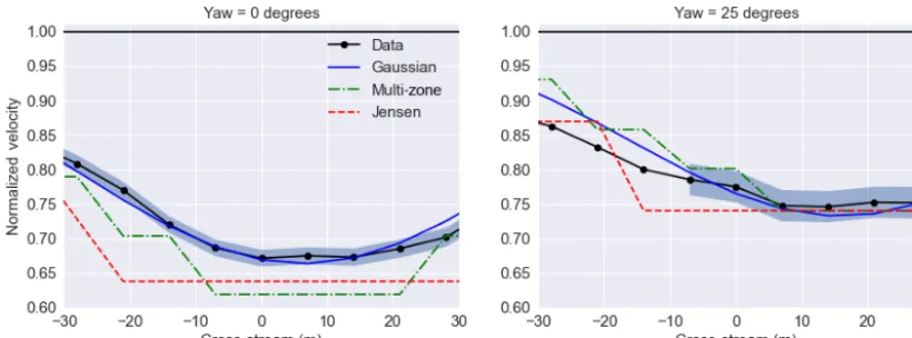
Figure 6 shows the comparison of each control-oriented engineering model with the lidar data when the turbine is op-erating with no misalignment (left) and opop-erating with 25◦ of yaw misalignment (right) at 180.95 m downstream, or
ap-proximately 2.5D downstream. Similar to Fig. 4, a “virtual” rotor is used to compute the effective wind speed at several spanwise locations. The data used in Fig. 6 include all tur-bulence intensity levels with wind speeds of 7–9 m s−1when the turbine was operating with no misalignment and a yaw misalignment of 25◦. The average turbulence intensity is
ap-proximately 7 %. The data were aggregated and normalized over this range of wind speeds to include more scans and pro-vide more robust statistics. The bands indicate a 95 % confi-dence interval.
Figure 6.Velocity deficit at 180.95 m downstream computed using lidar data, the Gaussian wake model, the multi-zone wake model, and the Jensen wake model under different yaw misalignment conditions.
the changing yaw angle; i.e., the thrust generated by the tur-bine is modified. This modified thrust is able to accommo-date the underpredictions in the normal operating case. With more data, the analysis could be split into yaw misalignment conditions and turbulence intensity levels.
5 Conclusions and future work
This paper compared field data from a scanning lidar mea-suring the wake of a turbine in normal operating condi-tions and yaw-misaligned condicondi-tions with control-oriented models. Validating these control models with field data in a variety of conditions is a critical step to implementing wind farm controls in the field. A quantitative analysis was done comparing the models in the FLORIS framework to these data. The data were processed to look at the effects of varying turbulence intensity levels as well as different yaw-misaligned conditions. The wake models used in the com-parison included the Jensen model, the multi-zone model, and the Gaussian wake mode. Future work will incorporate additional wake models that may be used in the context of wind farm controls. The Gaussian model provided the best representation of wake characteristics under different atmo-spheric conditions and different turbine operating conditions. Good agreement was also seen with the Jensen and multi-zone wake models on a smaller subset of data that matched the conditions of the tuning data.
Based on these results, this provides more confidence in wind farm controllers designed using these models. This study provided a first step towards validating these models in the field. In particular, this study focused on the wake of a single turbine. An increased understanding of these models at the wind farm level is needed to determine the potential performance of wind farm control solutions in the field.
Appendix A: FLORIS tuning values for near-wake lidar comparisons
Due to the limitations of the field data presented in this pa-per, FLORIS had to be tuned to capture the near wake be-hind the turbine. The wake was evaluated primarily at 2.35D (180.95 m) downstream. These parameters were tuned for 5 % turbulence intensity as indicated in the analysis. Below are the FLORIS tuning values for the near-wake lidar com-parisons shown in this paper.
– Jensen wake model
– ke=0.055 – kd=0.17
– For high turbulence cases (>10 % turbulence in-tensity),ke=0.1.
– Multi-zone wake model
– ke=0.1 – kd=0.17
– me= −0.5,0.3,1.0 – MU=0.47,1.28,5.5
– aU=11.7
– bU=0.72
– For high turbulence cases (>10 % turbulence in-tensity),ke=0.13.
– Gaussian wake model
– ka=0.17
Competing interests. The authors declare that they have no con-flict of interest.
Acknowledgements. The Alliance for Sustainable Energy, LLC (Alliance) is the manager and operator of the National Renewable Energy Laboratory (NREL). NREL is a national laboratory of the U.S. Department of Energy, Office of Energy Efficiency and Renewable Energy. This work was authored by the Alliance and supported by the U.S. Department of Energy under contract no. DE-AC36-08GO28308. Funding was provided by the U.S. Department of Energy Office of Energy Efficiency and Renewable Energy, Wind Energy Technologies Office. The views expressed in the article do not necessarily represent the views of the U.S. De-partment of Energy or the U.S. government. The U.S. government retains, and the publisher, by accepting the article for publication, acknowledges that the U.S. government retains a nonexclusive, paid-up, irrevocable, worldwide license to publish or reproduce the published form of this work, or allow others to do so, for U.S. government purposes.
Edited by: Raúl Bayoán Cal
Reviewed by: two anonymous referees
References
Abkar, M. and Porté-Agel, F.: Influence of atmospheric stability on wind-turbine wakes: A large-eddy simulation study, Phys. Fluids, 27, 035104, https://doi.org/10.1063/1.4913695, 2015.
Annoni, J., Gebraad, P. M., Scholbrock, A. K., Fleming, P. A., and Wingerden, J.-W. v.: Analysis of axial-induction-based wind plant control using an engineering and a high-order wind plant model, Wind Energy, 19, 1135–1150, https://doi.org/10.1002/we.1891, 2016.
Bastankhah, M. and Porté-Agel, F.: A new analytical model for wind-turbine wakes, Renew. Energ., 70, 116–123, 2014. Bastankhah, M. and Porté-Agel, F.: Experimental and theoretical
study of wind turbine wakes in yawed conditions, J. Fluid Mech., 806, 506–541, 2016.
Boersma, S., Doekemeijer, B., Gebraad, P., Fleming, P., Annoni, J., Scholbrock, A., Frederik, J., and van Wingerden, J.: A tutorial on control-oriented modeling and control of wind farms, in: Pro-ceedings of the American Control Conference (ACC), Seattle, USA, 2017.
Burton, T., Sharpe, D., Jenkins, N., and Bossanyi, E.: Wind energy handbook, John Wiley & Sons, 2001.
Campagnolo, F., Petrovi´c, V., Bottasso, C. L., and Croce, A.: Wind tunnel testing of wake control strategies, in: American Control Conference (ACC), 2016, 513–518, IEEE, 2016.
Chamorro, L. P. and Porté-Agel, F.: Turbulent flow inside and above a wind farm: a wind-tunnel study, Energies, 4, 1916–1936, 2011. Dilip, D. and Porté-Agel, F.: Wind Turbine Wake Mit-igation through Blade Pitch Offset, Energies, 10, 757, https://doi.org/10.3390/en10060757, 2017.
Fleming, P. A., Ning, A., Gebraad, P. M., and Dykes, K.: Wind plant system engineering through optimization of layout and yaw con-trol, Wind Energy, 19, 329–344, 2016.
Fleming, P., Annoni, J., Scholbrock, A., Quon, E., Dana, S., Schreck, S., Raach, S., Haizmann, F., and Schlipf, D.: Full-Scale Field Test of Wake Steering, Wake Conference, Visby, Sweden, 2017a.
Fleming, P., Annoni, J., Shah, J. J., Wang, L., Ananthan, S., Zhang, Z., Hutchings, K., Wang, P., Chen, W., and Chen, L.: Field test of wake steering at an offshore wind farm, Wind Energ. Sci., 2, 229–239, https://doi.org/10.5194/wes-2-229-2017, 2017b. Fleming, P. A., Gebraad, P. M., Lee, S., van Wingerden, J.-W.,
John-son, K., Churchfield, M., Michalakes, J., Spalart, P., and Mori-arty, P.: Evaluating techniques for redirecting turbine wakes us-ing SOWFA, Renew. Energ., 70, 211–218, 2014.
Fleming, P., Annoni, J., Churchfield, M., Martinez-Tossas, L. A., Gruchalla, K., Lawson, M., and Moriarty, P.: A simula-tion study demonstrating the importance of large-scale trail-ing vortices in wake steertrail-ing, Wind Energ. Sci., 3, 243–255, https://doi.org/10.5194/wes-3-243-2018, 2018.
Frandsen, S., Barthelmie, R., Pryor, S., Rathmann, O., Larsen, S., Højstrup, J., and Thøgersen, M.: Analytical modelling of wind speed deficit in large offshore wind farms, Wind Energy, 9, 39– 53, 2006.
Gebraad, P., Teeuwisse, F., Wingerden, J., Fleming, P., Ruben, S., Marden, J., and Pao, L.: Wind plant power optimization through yaw control using a parametric model for wake effects—a CFD simulation study, Wind Energy, 19, 95–114, 2016.
Gebraad, P. M. and Van Wingerden, J.: A control-oriented dynamic model for wakes in wind plants, J. Phys. Conf. Ser., 524, p. 012186, IOP Publishing, 2014.
Howland, M. F., Bossuyt, J., Martínez-Tossas, L. A., Meyers, J., and Meneveau, C.: Wake structure in actuator disk models of wind turbines in yaw under uniform inflow conditions, J. Renew. Sus-tain. Ener., 8, 043301, https://doi.org/10.1063/1.4955091, 2016. Jensen, N. O.: A note on wind generator interaction, Tech. Rep.
Risø-M-2411, Risø, 1983.
Jiménez, Á., Crespo, A., and Migoya, E.: Application of a LES tech-nique to characterize the wake deflection of a wind turbine in yaw, Wind Energy, 13, 559–572, 2010.
Johnson, K. E. and Thomas, N.: Wind farm control: Addressing the aerodynamic interaction among wind turbines, American Con-trol Conference, 2104–2109, 2009.
Johnson, K. E., Pao, L. Y., Balas, M. J., and Fingersh, L. J.: Con-trol of variable-speed wind turbines: standard and adaptive tech-niques for maximizing energy capture, IEEE Contr. Syst. Mag., 26, 70–81, 2006.
Jonkman, J.: NWTC Design Codes – FAST, https://nwtc.nrel.gov/ FAST (last access: September 2017), 2010.
Katic, I., Højstrup, J., and Jensen, N. O.: A simple model for cluster efficiency, in: European wind energy association conference and exhibition, 407–410, 1986.
Niayifar, A. and Porté-Agel, F.: A new analytical model for wind farm power prediction, J. Phys. Conf. Ser., 625, p. 012039, IOP Publishing, 2015.
Pope, S. B.: Turbulent flows, Cambridge university press, 2000. Raach, S., Schlipf, D., and Cheng, P. W.: Lidar-based wake tracking
for closed-loop wind farm control, J. Phys. Conf. Ser., 753, p. 052009, IOP Publishing, 2016.
for wind farm control, IFAC-PapersOnLine, 50, 4498–4503, 2017.
Schottler, J., Hölling, A., Peinke, J., and Hölling, M.: Wind tunnel tests on controllable model wind turbines in yaw, in: 34th Wind Energy Symposium, vol. 1523, 2016.
Smalikho, I., Banakh, V., Pichugina, Y., Brewer, W., Banta, R., Lundquist, J., and Kelley, N.: Lidar investigation of atmosphere effect on a wind turbine wake, J. Atmos. Ocean. Tech., 30, 2554– 2570, 2013.
Stanley, A. P., Thomas, J., Ning, A., Annoni, J., Dykes, K., and Fleming, P.: Gradient-Based Optimization of Wind Farms with Different Turbine Heights, in: 35th Wind Energy Symposium, p. 1619, 2017.
Stull, R. B.: An introduction to boundary layer meteorology, vol. 13, Springer Science & Business Media, 2012.
Thomas, J., Tingey, E., and Ning, A.: Comparison of two wake models for use in gradient-based wind farm layout optimization, in: Technologies for Sustainability (SusTech), 2015 IEEE Con-ference on, 203–208, IEEE, 2015.