Volume 2 | Issue 1
Article 2
2015
Bayesian Spam Detection
Jeremy J. Eberhardt
University or Minnesota, Morris
Follow this and additional works at:
http://digitalcommons.morris.umn.edu/horizons
This Article is brought to you for free and open access by University of Minnesota Morris Digital Well. It has been accepted for inclusion in Scholarly Horizons: University of Minnesota, Morris Undergraduate Journal by an authorized administrator of University of Minnesota Morris Digital Well. For more information, please [email protected].
Recommended Citation
Eberhardt, Jeremy J. (2015) "Bayesian Spam Detection,"Scholarly Horizons: University of Minnesota, Morris Undergraduate Journal: Vol. 2: Iss. 1, Article 2.
Bayesian Spam Detection
Jeremy Eberhardt
Division of Science and Mathematics University of Minnesota, Morris Morris, Minnesota, USA 56267
[email protected]
ABSTRACT
Spammers always find new ways to get spammy content to the public. Very commonly this is accomplished by using email, social media, or advertisements. According to a 2011 report by the Messaging Anti-Abuse Working Group roughly 90% of all emails in the United States are spam. This is why we will be taking a more detailed look at email spam. Spam filters have been getting better at detecting spam and removing it, but no method is able to block 100% of it. Because of this, many different methods of text classification have been developed, including a group of classifiers that use a Bayesian approach. The Bayesian approach to spam filtering was one of the earliest methods used to filter spam, and it remains relevant to this day.
In this paper we will analyze 2 specific optimizations of Naive Bayes text classification and spam filtering, looking at the differences between them and how they have been used in practice. This paper will show that Bayesian filtering can be simply implemented for a reasonably accurate text classifier and that it can be modified to make a significant impact on the accuracy of the filter. A variety of applications will be explored as well.
Keywords
Spam, Bayesian Filtering, Naive Bayes, Multinomial Bayes, Multivariate Bayes
1.
INTRODUCTION
It is important to be able to detect spam emails not only for personal convenience, but also for security. Being able to remove emails with potential viruses or malicious software of any kind is important on individual user levels and larger scales.
Bayesian text classification has been used for decades, and it has remained relevant throughout those years of change. Even with newer and more complicated methods having been developed, Naive Bayes, also called “Idiot Bayes” for its simplicity, still matches and even outperforms those newer
This work is licensed under the Creative Commons Attribution-Noncommercial-Share Alike 3.0 United States License. To view a copy of this license, visit http://creativecommons.org/licenses/by-nc-sa/3.0/us/ or send a letter to Creative Commons, 171 Second Street, Suite 300, San Fran-cisco, California, 94105, USA.
UMM CSci Senior Seminar Conference, December 2014Morris, MN.
methods in some cases. There are many modifications that can be made to Naive Bayes, which demonstrates the mas-sive scope of Bayesian classification methods.
Most commonly used in email spam filtering, Naive Bayes can be used to classify many different kinds ofdocuments. A document is anything that is being classified by the filter. In our case, we will primarily be discussing the classification of emails. One further application will be explored in sec-tion 8.1. The class of a document in our case is very simple: something will be classified as eitherspamorham. Spam is an unwanted document and ham is a non-spam document.
All of the methods discussed here usesupervised forms of machine learning. This means that the filter that is created first needs to be trained by previously classified documents provided by the user. Essentially this means that you cannot develop a filter and immediately implemented it, because it will not have any basis for classifying a document as spam or ham. But once you do train the filter, no more training is needed as each new document classified additionally trains the filter by simply being classified. There are other imple-mentations that aresemi-supervised, where documents that have not been explicitly classified can be used to classify further documents. But in the following models, all docu-ments that are classified or in the training data are classified as either spam or ham, not using any semi-supervised tech-niques.
Three methods of Bayesian classification will be explored, those beingNaive Bayes,Multinomial Bayes, and Multivari-ate Bayes. Multinomial Bayes and Multivariate Bayes will be analyzed in more detail due to their more practical ap-plications.
2.
BAYESIAN NETWORKS
A Bayesian network is a representation of probabilistic relationships. These relationships are shown usingDirected Acyclic Graphs(DAGs). DAGs are graphs consisting of ver-tices and directed edges wherein there are no cycles. Each node is a random variable. Referencing figure 1, the prob-ability of a node occurring is the product of the probabil-ity that the random variable in the node occurs given that the parents have occurred. This can also be shown with the following equation. P(x1, ..., xn) is the probability of
any node xi and P a(xi) is the probability of the parent.
P(xi|P a(xi)) is also called aconditional probability,
mean-ing that the probability of an event is directly affected by the occurrence of another event. [8]
P(x1, ..., xn) =
Y
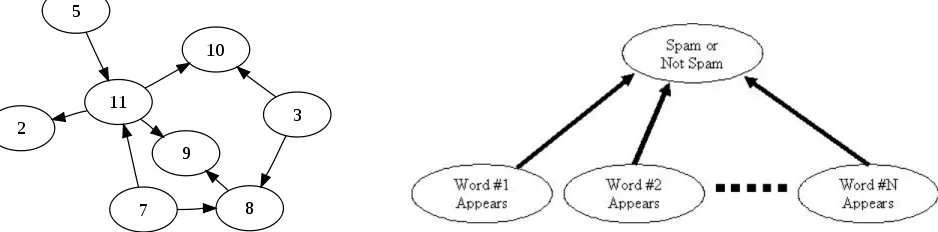
Figure 1: A simple Bayesian network. Note that there is no way of cycling back to any node.
In our case, each node is afeaturethat is found in a docu-ment. A feature is any element of a document that is being used to classify the document. Features can be words, seg-ments of words, lengths of words, or any other element of a document. Using these nodes and formula 1, one can find the probability that an email (document) is spam given all of the words (features) found in the email. This idea will be explored further in the following sections. These graphs can also be used to determine independence of random variables. For example, in figure 1 node 5 is completely independent of all other nodes. Node 5 does not have any parents, so there are no dependencies. Node 11, however, is dependent upon both node 5 and node 7. In this manner one can determine the dependence and independence of any random variable in the DAG. This is an abstract way to view how Bayesian sta-tistical filtering is done. Bayesian networks and the formula above rely heavily on the fact that the nodes have dependen-cies. The models discussed in this paper, however, arenaive, meaning that instead of assuming dependencies they assume that all features (nodes) are completely independent from one another. They use the same idea of Bayesian networks, but simplify it to create a relatively simple text classifier. Figures 1 and 2 demonstrate the differences visually.
3.
NAIVE BAYES
Naive Bayes spam detection is a common model to detect spam, however it is seldom used in the following implemen-tation. Most Bayesian spam filters use an optimization of Naive Bayes which will be covered in sections 4 and 5. Naive Bayes must be trained with controlled data that is already defined as spam or ham so the model can be applied to real-world situations. Naive Bayes also assumes that the fea-tures that it is classifying, in our case the individual words of the email, are independent from one another. Addition-ally, adjustments can be made not only to the Naive Bayes algorithm of classification, but also the methodology used to choose features that will be analyzed to determine the class of a document, which will be discussed further in section 6. Once the data is given, a filter is created that assigns the probability that each feature is in spam. Probabilities in this case are written as values between 0 and 1. Common words such as “the” and “it” will be assigned very neutral proba-bilities (around 0.5). In many cases, these words will simply be ignored by the filter, as they offer very little relevant in-formation. Now that the filter is ready to detect spam from the training data, it will evaluate whether or not an email
Figure 2: A visualization of the Naive Bayes model.
is spam based on the individual probabilities of each word. Figure 2 shows that the words are independent from each other in the classification of the email, and are all treated equally. Now we have nearly everything we need to classify an email. Below is a formula for P(S|W), the probability than an email is spam given that word W is in the email. This is also called thespamicity of a word.
P(S|W) = P(W|S)·P(S)
P(W|S)·P(S) +P(W|H)·P(H) [10] (2) W represents a given word, S represents a spam email and H represents a ham email. The left side of the equation can be read as “The probability that an email is spam given that the email contains word W.”P(W|S) andP(W|H) are the conditional probabilities of the word W. For P(W|S), this would be the proportion of spam documents that also contain word W. P(W|H), similarly, is the proportion of ham documents that also contain wordW. These probabili-ties come from the training data. P(S) the probability that any given email is spam andP(H) the probability that any given email is ham vary depending on the approach. Some use the current probability that any given email is spam. Currently, it is estimated that around 80%-90% of all emails are spam [1]. There are also some approaches that choose to assume there is no previous assumption aboutP(S), so they choose to use an even 0.5. Another approach is to use the data from the training set used to train the filter, which makes the filter more tailored for the user since the user classified the training data.
To combine these probabilities we can use the following formula.
P(S|W) = P1P2...PN
P1P2...PN+ (1−P1)(1−P2)...(1−PN)
[10]
(3) Wdenotes a set of words, soP(S|W) is the probability that a document is spam given that a set of wordsWoccur in the document. N is the total number of features that were classified. In the context of email spam, N would be the total number of words contained in the email. P1...PN
are spamicities of each individual word in the email, which can also be represented asP(S|W1)...P(S|WN).
Using such a small data set is not likely to give you a very ac-curate probability, but using documents with a much larger set of words will yield a more accurate result. Now we would likely compare 0.034 to a pre-determined threshold or to P(H|W) calculated similarly, which would ultimately label the document as either spam or ham.
4.
MULTINOMIAL NAIVE BAYES
Multinomial Bayes is an optimization that is used to make the filter more accurate. In essence we perform the same steps, but this time we keep track of the number of oc-currences of each word. So for the following formulas W represents amultisetof words in the document. This means thatW also contains the correct number of occurrences of each word. For purposes of further application, one way to represent Naive Bayes using Bayes theorem and the law of total probability is
P(S|W) = PP(W|S)·P(S)
SP(S)·P(W|S)
[4] (4)
Recall thatWis a multiset of words that occur in a docu-ment and S means that the docudocu-ment is spam. For example, if a document had words A, B, C, and C again as its contents, Wwould be (A, B, C, C). Note that duplicates are allowed in the multiset. Since we now have Naive Bayes written out this way, we can expand it to assume that the words are generated following a multinomial distribution and are in-dependent. Note that identifying an email as spam or ham is binary, we know that our class can only ever be 0 or 1, S or H. With those assumptions, we can now write our Multi-nomial Bayes equation as
P(W|S) = (
P
WfW)!
Q
WfW!
Y
W
P(W|S)fW [4] (5)
wherefWis the number of times that the word W takes place
in the multisetW and Q
W is the product for each word
in W. This formula can be further manipulated, for the alternative formula and its derivation see Freeman’sUsing Naive Bayes to Detect Spammy Names in Social Networks. [4]
We now have everything we need except forP(W|S): the probability that a given word occurs in a spam email. This can be estimated using the training data provided by the user. In the following equation αW,S is the smoothing
pa-rameter. It prevents this value from being 0 if there are few occurrences of a particular word. In doing so it prevents our calculation from being highly inaccurate. It also prevents a divide-by-zero error. Usually, this number is set to 1 for all αW,S, which is calledLaplace smoothing. This results in the
smallest possible impact on the value while simultaneously avoiding errors. Our formula is
P(W|S) = NW,S+αW,S NS+PWαW,S
[4] (6)
where NW,S is the number of occurrences of a word W in
a spam email. NS is the total number of words that have
been found in the spam emails up to this point by the filter. This number will grow as more emails are added to the filter that are classified as spam and that contain new words.
Now that each of the parameters have a value, you simply use our initial equation 4 and find the probability. In our
case of email spam detection, it is most likely that the cal-culated probability would be compared to a certain thresh-old that is given by the user to classify the email as either spam or ham. The resulting value could also be compared toP(H|W), which can be calculated similarly toP(S|W). The class of the email would be decided by the maximum of the two values. Note that Multinomial Bayes does not scale well to large documents where there is a higher likelihood of duplicate features due to the calculation time.
5.
MULTIVARIATE NAIVE BAYES
Multivariate Naive Bayes, also known asBernoulli Naive Bayes is a method that is closely related to Multinomial Bayes. Similar to the multinomial approach, it treats each feature individually. However, they are treated asbooleans.[9]. This means that W contains either true or false for each word, instead of containing the words themselves. W con-tains A elements, where A is the number of elements in the
vocabulary. The vocabulary is a set of each unique word that has occurred in the training data. Each element is true or false, and each correspond to a particular word. Note that Multivariate Bayes is still naive, so each feature is still independent from all other features. We can find the proba-bilities of the parameters in a similar fashion to Multinomial Bayes, resulting in the following equation:
P(W|S) = 1 +NW,S 2 +NS
[9]
Note that this multivariate equation of classification also implements smoothing of 1 in the numerator and 2 in the denominator to prevent the filter from assigning a 1 or 0 to certain words. NW,S is the total number of training spam
documents that contain the word W and NS is the total
number of training documents that are classified as spam. Multivariate Bayes does not keep track of the number of occurrences of features, unlike Multinomnial Bayes, which means that Multivariate Bayes scales better. The total prob-ability of the document can be calculated in the same way as Multinomial Bayes using equation 4 using our newW.
6.
FEATURE SELECTION
For Naive Bayes, the method for determining the rele-vance of any given word is quite complex. Bayesian feature selection only works if we assume that features are indepen-dent from each other and we can assume future occurrences of spam will be similar to past occurrences of spam. The filter assigns each word a probability of being contained in a spam email. This is done by using the following formula for a given wordW:
P(W) =
NW,S NS
NW,H
NH +
NW,S
NS
NW,Sis the number of times that word W occurs in spam
documents,NW,H is the number of time that word W occurs
in ham documents, NS is the total number of spam
docu-ments andNH is the total number of ham documents. For
for being considered relevant can vary per user, as there is not one perfect threshold.[2]
As demonstrated by Freeman [4], adjustments can be made to feature selection to more appropriately suit the given data. One example of this is given by Freeman. In Free-man’s case, the author was using words to determine valid names for LinkedIn. LinkedIn is a social networking service designed for people looking for career networking or oppor-tunities. Since names are only ever a few words long, using individual words for text classification would not be ade-quate. N-grams, or sections of words, allow Bayesian meth-ods to be applied. Each word was broken up into 3 letter segments. For example, the name “David” would be broken up into (\^Da,dav,avi,vid,id\$). \ˆ and\$ represent the be-ginning and end of a word, respectively. Then the Bayesian filter would classify each of those individual n-grams with different levels of spamicity. Recall that the spamicity of a word isP(S|W), the probability that a document is spam given that word W occurs in the document. In our case, W is an n-gram instead of a word. This can be applied to things other than n-grams, for example a certain length of a word can have a spamicity. W can be any desired fea-ture. It is important to note that using n-grams breaks a key assumption of Naive Bayes: the features are no longer independent from each other. However, results indicated that it was still possible to have reliable outcomes, although it was also possible to have highly inaccurate outcomes. [4] Additionally, individual aspects of the document may be given more weight than others. For example, in an email the contents of the subject line may be given more weight than body of the email. This particular adjustment of feature selection will not be explored in detail in this paper, how-ever, it is important to note that there are many different ways that feature selection can be implemented which vary depending on the type of document that is being classified.
7.
ADVANTAGES AND DISADVANTAGES
Naive Bayes is a very simple algorithm that performs equally well against much more complex classifiers in many cases, and even occasionally outperforms them. It also does not classify the email on the basis of one or two words, but instead takes into account every single relevant word. For example, if the word “cash” has a high probability of being in a spam email and the word “Charlie” has a low probability of being in a spam email and they both occur in the same email, they will cancel each other out. In that way, it does not make premature classifications of the email.
Another benefit of Bayesian filtering is that it is constantly adapting to new forms of spam. This means that as the filter is identifying spam and ham, it adds that data to its filter and applies it to later emails. One documented example of this is from GFI Software [2]. Spammers began to use the word “F-R-E-E” instead of “FREE”. Once “F-R-E-E” was added to the database of keywords by the filter, it was able to successfully filter out spam emails containing that word. [3, 6]
Bayesian filtering can also be tailor-made to individual users. The filter depends entirely upon the training data that is provided by the user, which is classified into spam and ham prior to training the model. In addition, adjust-ments can be made not only to the Naive Bayes algorithm of classification, but also the methodology used to choose features that will be analyzed to determine the class of a
document as previously discussed. However, this is also one of the most significant disadvantages of Bayesian filtering as well. Regardless of the method that you use, you will need to provide training data to the model. Not only does this make it difficult to train the model precisely, but it also takes time depending on the size of the training data.
There have also been instances of Bayesian poisoning. Bayesian poisoning is when a spammer intentionally includes words or phrases that are specifically designed to trick a Bayesian filter into believing that the email is not spam. These words and phrases can be completely random, this would tilt the spamicity level of the email slightly more fa-vorably towards non-spam. However, some spammers ana-lyze data to specifically find words that are not simply neu-tral, but actually are more commonly found in non-spam. Of course, over time, the filter will adapt to these new spam-mers and catch them. All of this takes time, which can be an important variable when choosing a classifier. [5]
It is also subject to spam images. Unless the filter is specifically designed with image detection in mind, it is hard for the filter to recognize when an image is spam or not, so in many cases it is ignored. This makes it possible for the spammer to use an image with the spam message in it as the email message.
8.
TESTING AND RESULTS
8.1
Multinomial Bayes
Freeman ran his Multinomial Bayes classifier on account names on the social media and networking site LinkedIn. Specifically, this testing was done using Multinomial Bayes and n-grams. N-grams were used because account names are only ever a few words long, and with varying size n-grams. N-grams of a string in his experiment were defined as the (m−n+ 1) substring of a string of length m represented as (c1c2...cm). n-grams of a word W can be written as:
(c1c2...cn, c2c3...cn+1, ..., cm−n+1cm−n+2...cm). n is chosen
for the desired size of the n-grams. Freeman used n = 1 throughn= 5 for 5 separate trials.
The data was trained with 60 million LinkedIn accounts that were already identified as either good standing or bad standing initially. They then chose about 100,000 accounts to test the classifier on. Roughly 50,000 were known to be spam and 50,000 were known to be ham from the validation set. After some trials, it was determined that the values n = 3 and n = 5 were the most effective for the memory trade-offs. The higher the n, the more memory that the classifier used. Storing n= 3 n-grams used approximately 110 MB of distinct memory, whereas n = 5 n-grams used about 974 MB. As you can see, the rate of memory required grows rapidly, which is why n = 5 was the highest value used in the trials.
clas-Figure 3: A graph of the accuracy of the lightweight and full Multinomial Bayes name spam detection al-gorithm by Freeman. [4]
sifier increased accuracy of identifying spammy names on LinkedIn are shown in figure 3. In the graph, the two lines represent the two algorithms that were used. The “full” algo-rithm isn= 5 and the “lightweight” algorithm isn= 3. The lightweight algorithm gets less accurate faster than the full algorithm, but the lightweight algorithm was deemed better for smaller data sets due to the smaller memory overhead. Both are accurate, but the full algorithm was consistently more accurate.
The algorithm was run on live data and reduced the false positive rate of the algorithm (previously based on regular expressions) from 7% to 3.3%. Soon after it completely re-placed the old algorithm. [4]
8.2
Multivariate Bayes
Multivariate Bayes has proven to be one of the least accu-rate Bayesian implementations for document classification. However, it is still surprisingly accurate for its simplicity. It treats its features as only booleans, meaning that either a feature exists in a document or it does not exist in doc-ument. Given only that information, it averaged around a 89% accuracy rating by Metsis [9]. While it is not the most accurate implementation, it is still applicable to individual user situations, as it is far simpler than many other clas-sifiers and still does an adequate job of filtering out spam messages.
In the graph above, the y-axis is the true positive rate, and the x-axis is the false positive rate. Multivariate Bayes yields more false positive rates as the true positive rate in-creases than Multinomial Bayes. In this study, at total of 6 Naive Bayes methods were tested. Note that the graph above is an approximation, for the full graph (including the other Naive Bayes methods), see [7]. The Multinomial Bayes performed the best of all of the methods used in these tests, and Multivariate performed the worst. This testing set was generated using data gathered fromEnron emails as ham,
Figure 4: Multivariate Bayes positive rates com-pared to Multinomial Bayes positive rates. [7]
and mixed in generic non-personal spam emails. This data was used with varying numbers of feature sets. In figure 4, 3000 features were used per email to classify it. As the graph demonstrates, this particular Bayesian method is not the most effective in this case. [7]
9.
CONCLUSIONS
In this paper we have analyzed 2 different methods of Naive Bayes text classification in the context of spam de-tection. We have also discussed possible modifications to the feature selection process in increase the accuracy of the filters. Bayesian text classification can be applied to a mul-titude of applications, 2 of which were explored here. Most importantly, it has been observed that Bayesian methods of text classification are still relevant today, even with new and more complex methods having been developed and tested. Minor modifications can make significant differences in ac-curacy, and finding the modifications that increase accuracy for a particular environment is the key to making Bayesian methods effective.
10.
ACKNOWLEDGMENTS
Thank you Elena Machkasova and Chad Seibert, for your excellent feedback and recommendations.
11.
REFERENCES
[1] Messaging anti-abuse working group report: First, second and third quarter 2011. November 2011. [2] Why bayesian filtering is the most effective anti-spam
technology. 2011.
[3] S. Abu-Nimeh, D. Nappa, X. Wang, and S. Nair. A comparison of machine learning techniques for
[4] D. M. Freeman. Using naive bayes to detect spammy names in social networks. InProceedings of the 2013 ACM Workshop on Artificial Intelligence and
Security, AISec ’13, pages 3–12, New York, NY, USA, 2013. ACM.
[5] L. Huang, A. D. Joseph, B. Nelson, B. I. Rubinstein, and J. D. Tygar. Adversarial machine learning. In
Proceedings of the 4th ACM Workshop on Security and Artificial Intelligence, AISec ’11, pages 43–58, New York, NY, USA, 2011. ACM.
[6] B. Markines, C. Cattuto, and F. Menczer. Social spam detection. InProceedings of the 5th International Workshop on Adversarial Information Retrieval on the Web, AIRWeb ’09, pages 41–48, New York, NY, USA, 2009. ACM.
[7] V. Metsis, I. Androutsopoulos, and G. Paliouras. Spam filtering with naive bayes - which naive bayes? InCEAS, 2008.
[8] I. Shmulevich and E. Dougherty.Probabilistic Boolean Networks: The Modeling and Control of Gene Regulatory Networks. Society for Industrial and Applied Mathematics. Society for Industrial and Applied Mathematics, 2010.
[9] V. M. Telecommunications and V. Metsis. Spam filtering with naive bayes – which naive bayes? In
Third Conference on Email and Anti-Spam (CEAS, 2006.