Improved representation of plant functional types and physiology in the Joint UK Land Environment Simulator (JULES v4.2) using plant trait information

(1)

www.geosci-model-dev.net/9/2415/2016/ doi:10.5194/gmd-9-2415-2016

Improved representation of plant functional types and physiology in

the Joint UK Land Environment Simulator (JULES v4.2) using

plant trait information

Anna B. Harper1, Peter M. Cox1, Pierre Friedlingstein1, Andy J. Wiltshire2, Chris D. Jones2, Stephen Sitch3, Lina M. Mercado3,4, Margriet Groenendijk3, Eddy Robertson2, Jens Kattge5, Gerhard Bönisch5, Owen K. Atkin6, Michael Bahn7, Johannes Cornelissen8, Ülo Niinemets9,10, Vladimir Onipchenko11, Josep Peñuelas12,13,

Lourens Poorter14, Peter B. Reich15,16, Nadjeda A. Soudzilovskaia17, and Peter van Bodegom17

1_{College of Engineering, Mathematics, and Physical Sciences, University of Exeter, Exeter, UK} 2_{Met Office Hadley Centre, Exeter, UK}

3_{College of Life and Environmental Sciences, University of Exeter, Exeter, UK} 4_{Centre for Ecology and Hydrology, Wallingford, UK}

5_{Max Planck Institute for Biogeochemistry, Jena, Germany}

6_{ARC Centre of Excellence in Plant Energy Biology, Research School of Biology, Australian National University,}

Canberra, Australia

7_{Institute of Ecology, University of Innsbruck, Austria}

8_{Systems Ecology, Department of Ecological Science, Vrije Universiteit, Amsterdam, the Netherlands} 9_{Institute of Agricultural and Environmental Sciences, Estonian University of Life Sciences, Tartu, Estonia} 10_{Estonian Academy of Sciences, Tallinn, Estonia}

11_{Department of Geobotany, Moscow State University, Moscow 119234, Russia}

12_{CSIC, Global Ecology Unit CREAF-CSIC-UAB, Cerdanyola del Vallès, 08193 Barcelona, Catalonia, Spain} 13_{CREAF, Cerdanyola del Vallès, 08193 Barcelona, Catalonia, Spain}

14_{Forest Ecology and Forest Management Group, Wageningen University, P.O. Box 6700 AA, Wageningen, the Netherlands} 15_{Department of Forest Resources, University of Minnesota, Saint Paul, Minnesota, USA}

16_{Hawkesbury Institute for the Environment, University of Western Sydney, Penrith, New South Wales, Australia} 17_{Institute of Environmental Sciences, Leiden University, Leiden, the Netherlands}

Correspondence to:Anna B. Harper ([email protected])

Received: 27 January 2016 – Published in Geosci. Model Dev. Discuss.: 1 February 2016 Revised: 13 May 2016 – Accepted: 20 May 2016 – Published: 22 July 2016

Abstract. Dynamic global vegetation models are used to predict the response of vegetation to climate change. They are essential for planning ecosystem management, under-standing carbon cycle–climate feedbacks, and evaluating the potential impacts of climate change on global ecosystems. JULES (the Joint UK Land Environment Simulator) repre-sents terrestrial processes in the UK Hadley Centre fam-ily of models and in the first generation UK Earth System Model. Previously, JULES represented five plant functional types (PFTs): broadleaf trees, needle-leaf trees, C3 and C4

grasses, and shrubs. This study addresses three developments

in JULES. First, trees and shrubs were split into deciduous and evergreen PFTs to better represent the range of leaf life spans and metabolic capacities that exists in nature. Second, we distinguished between temperate and tropical broadleaf evergreen trees. These first two changes result in a new set of nine PFTs: tropical and temperate broadleaf evergreen trees, broadleaf deciduous trees, needle-leaf evergreen and decid-uous trees, C3and C4grasses, and evergreen and deciduous

(2)

turnover and growth rates to include a trade-off between leaf life span and leaf mass per unit area.

Overall, the simulation of gross and net primary produc-tivity (GPP and NPP, respectively) is improved with the nine PFTs when compared to FLUXNET sites, a global GPP data set based on FLUXNET, and MODIS NPP. Compared to the standard five PFTs, the new nine PFTs simulate a higher GPP and NPP, with the exception of C3grasses in cold

environ-ments and C4grasses that were previously over-productive.

On a biome scale, GPP is improved for all eight biomes eval-uated and NPP is improved for most biomes – the excep-tions being the tropical forests, savannahs, and extratropical mixed forests where simulated NPP is too high. With the new PFTs, the global present-day GPP and NPP are 128 and 62 Pg C year−1, respectively. We conclude that the inclusion of trait-based data and the evergreen/deciduous distinction has substantially improved productivity fluxes in JULES, in particular the representation of GPP. These developments in-crease the realism of JULES, enabling higher confidence in simulations of vegetation dynamics and carbon storage.

1 Introduction

The net exchange of carbon dioxide between the vegetated land and the atmosphere is predominantly the result of two large and opposing fluxes: uptake by photosynthesis and ef-flux by respiration from soils and vegetation. CO2can also

be released by land ecosystems due to vegetation mortal-ity resulting from human and natural disturbances, such as changes in land use practices, insect outbreaks, and fires. Vegetation models are used to quantify many of these fluxes, and the evolution of the terrestrial carbon sink strongly af-fects future greenhouse gas concentrations in the atmosphere (Friedlingstein et al., 2006; Friedlingstein, 2015; Arora et al., 2013). A subset of vegetation models also predicts both compositional and biogeochemical responses of vege-tation to climate change (dynamic global vegevege-tation models, DGVMs), one of these being the Joint UK Land Environ-ment Simulator (JULES). ) (Best et al., 2011; Clark et al., 2011). JULES predecessor, the Met Office Surface Exchange Scheme (MOSES: Cox et al., 1998, 1999; Essery et al., 2001, 2003) was the land component of the Hadley Centre Global Environmental Model (HadGEM2), and JULES will repre-sent the land surface in the next generation UK Earth Sys-tem Model (UKESM). Within JULES, the TRIFFID model (Top-down Representation of Foliage and Flora Including Dynamics; Cox, 2001) predicts changes in biomass and the fractional coverage of five plant functional types (PFTs; broadleaf trees, needle-leaf trees, C3 grass, C4 grass, and

shrubs) based on cumulative carbon fluxes and a predeter-mined dominance hierarchy. DGVMs such as JULES are es-sential for planning ecosystem management, understanding carbon cycle–climate feedbacks, and evaluating the potential

Table 1.Parameters used for the five PFT experiment (JULES5). The standard PFTs are broadleaf trees (BT), needle-leaf trees (NT), C3grass, C4grass, and shrubs (SH).Nmwas calculated by dividing the defaultNl0byCmass(0.5 in this study), LMA was calculated as σL×Cmass, andsvwas calculated to yield the sameVcmax,25as with the default five PFTs. All other parameters were taken from Clark et al. (2011). Parameters are defined in Table A1.

BT NT C3 C4 SH

awl 0.65 0.65 0.005 0.005 0.10

Dcrit 0.09 0.06 0.10 0.075 0.10

dT 9 9 9 9 9

f0 0.875 0.875 0.900 0.800 0.900

fd 0.010 0.015 0.015 0.025 0.015

iv 0 0 0 0 0

Lmax 9 6 4 4 4

Lmin 1 1 1 1 1

LMA 0.075 0.200 0.050 0.100 0.100

N_a∗ 1.73 3.30 1.83 3.00 3.00

Nm 0.023 0.0165 0.0365 0.030 0.030

rootd 3 1 0.5 0.5 0.5

sv 21.33 8.00 32.00 8.00 16.00

Tlow 0 −10 0 13 0

Toff 5 −40 5 5 5

Topt 32 22 32 41 32

Tupp 36 26 36 45 36

Vcmax,25 36.8 26.4 58.4 24.0 48.0

α 0.08 0.08 0.12 0.06 0.08

γ0 0.25 0.25 0.25 0.25 0.25

γp 20 15 20 20 15

µrl 1.0 1.0 1.0 1.0 1.0

µsl 0.10 0.10 1.00 1.00 0.10

∗_{These are derived from other parameters. Here}_N

ais g N m−2.

impacts of climate change on global ecosystems. However, the use of DGVMs in ESMs is relatively rare. For example, of the nine coupled carbon cycle–climate models evaluated by Arora et al. (2013), only three distinct DGVMs interac-tively simulated changes in the spatial distribution of PFTs (the spatially explicit individual-based (SEIB)-DGVM, JS-BACH (the Jena Scheme for Biosphere–Atmosphere Cou-pling in Hamburg), and JULES/TRIFFID).

(3)

(a) (b)

(c) (d)

Figure 1.Trade-offs between leaf mass per unit area (LMA; kg m−2)and(a, c)leaf nitrogen (g g−1), and between LMA and(b, d)leaf life span (LL).(a, b)Parameters in the standard JULES, converted fromNl0andσlbased on 0.4 kg C per kg dry mass (assumed parameter in JULES from Clark et al., 2011).(c, d)Median values from the TRY database for the new nine PFTs. In(b)and(d), the filled circles show the observed data and the open shapes show the median values from global simulations of JULES from 1982 to 2012. Vertical and horizontal lines show the range of vales between the lower and upper quartile of data.

Based on these previous results, our study addressed three potential improvements in the parameterization and repre-sentation of PFTs in JULES. First, the original five PFTs (Table 1) did not represent the range of leaf life spans and metabolic capacities that exists in nature, and so trees and shrubs were split into deciduous and evergreen PFTs. In a broad sense, the differences between evergreen and decidu-ous strategies can be summarized in a leaf economics spec-trum, where leaves employ trade-offs in their nitrogen use (Reich et al., 1997; Wright et al., 2004; Fig. 1). When pho-tosynthesis is limited by CO2, the photosynthetic capacity of

a leaf is dependent on the maximum rate of carboxylation of Rubisco (Vcmax). Plants allocate about 10–30 % of their

nitrogen into synthesis and maintenance of Rubisco (Evans, 1989), while a portion of the remaining nitrogen is put to-ward leaf structural components, and hence the strong re-lationship between photosynthetic capacity and leaf nitro-gen concentration (e.g., Meir et al., 2002; Reich et al., 1998; Wright et al., 2004) and leaf structure (Niinemets, 1999). On average, evergreen species have a lower photosynthetic ca-pacity and respiration per unit leaf mass (Reich et al., 1997; Wright et al., 2004; Takashima et al., 2004), higher leaf mass

per unit area (LMA) (Takashima et al., 2004; Poorter et al., 2009), allocate a lower fraction of leaf N to photosynthesis (Takashima et al., 2004), and exhibit lower N loss at senes-cence (Aerts, 1995; Silla and Escudero, 2003; Kobe et al., 2005) than deciduous species. There is also a positive rela-tionship between LMA and leaf life span (Reich et al., 1992, 1997; Wright et al., 2004). Leaves with high nutrient concen-tration tend to have a short life span and low LMA. They are able to allocate more nutrients to photosynthetic machinery to rapidly assimilate carbon at a relatively high rate (but they also have high respiration rates). Conversely, leaves with less access to nutrients use a longer-term investment strategy, al-locating nutrients to structure, defense, and tolerance mech-anisms. They tend to have longer life spans, low assimilation and respiration rates, but high LMAs.

Second, we distinguished between tropical broadleaf ev-ergreen trees and broadleaf evev-ergreen trees from warm-temperate and Mediterranean climates, based on fundamen-tal differences in leaf traits, chemistry, and metabolism (Ni-inemets et al., 2007, 2015; Xiang et al., 2013). For example, measuredVcmaxfor a given leaf N per unit area (NA)can be

(4)

Table 2.Updated parameters used in JULES9_ALL. The new PFTs are tropical broadleaf evergreen trees (BET-Tr), temperate broadleaf evergreen trees (BET-Te), needle-leaf evergreen trees (NET), needle-leaf deciduous trees (NDT), C3grass, C4grass, evergreen shrubs (ESh), and deciduous shrubs (DSh).

BET-Tr BET-Te BDT NET NDT C₃ C₄ ESh DSh

awl 0.65 0.65 0.65 0.65 0.75 0.005 0.005 0.10 0.10

Dcrit 0.090 0.090 0.090 0.060 0.041 0.051 0.075 0.037 0.030

dT 9 9 9 9 9 0 0 9 9

f₀ 0.875 0.892 0.875 0.875 0.936 0.931 0.800 0.950 0.950

fd 0.010 0.010 0.010 0.015 0.015 0.019 0.019 0.015 0.015

iv 7.21 3.90 5.73 6.32 6.32 6.42 0.00 14.71 14.71

Lmax 9 7 7 7 6 3 3 4 4

Lmin 1 1 1 1 1 1 1 1 1

LMA 0.1039 0.1403 0.0823 0.2263 0.1006 0.0495 0.1370 0.1515 0.0709

N_a∗ 1.76 2.02 1.74 2.61 1.87 1.19 1.55 2.04 1.54

Nm 0.017 0.0144 0.021 0.0115 0.0186 0.0240 0.0113 0.0136 0.0218

rootd 3 2 2 1.8 2 0.5 0.5 1 1

sv 19.22 28.40 29.81 18.15 23.79 40.96 20.48 23.15 23.15

Tlow 13 13 5 5 −5 10 13 10 0

Toff 0 −40 5 −40 5 5 5 −40 5

Topt 39 39 39 33 34 28 41 32 32

Tupp 43 43 43 37 36 32 45 36 36

Vcmax,25 41.16 61.28 57.25 53.55 50.83 51.09 31.71 62.41 50.40

α 0.08 0.06 0.08 0.08 0.10 0.06 0.04 0.06 0.08

γ₀ 0.25 0.50 0.25 0.25 0.25 3.0 3.0 0.66 0.25

γp 15 15 20 15 20 20 20 15 30

µrl 0.67 0.67 0.67 0.67 0.67 0.72 0.72 0.67 0.67

µsl 0.10 0.10 0.10 0.10 0.10 1.00 1.00 0.10 0.10

∗_{These are derived from other parameters. Here}_N

ais g N m−2.

evergreen trees (Kattge et al., 2011), resulting in lowerVcmax

and maximum assimilation rates for tropical forests (Car-swell et al., 2000; Meir et al., 2002, 2007; Domingues et al., 2007, 2010; Kattge et al., 2011). Collectively, the ever-green/deciduous and tropical/temperate distinctions resulted in a new set of nine PFTs for JULES: tropical broadleaf ev-ergreen trees (BET-Tr), temperate broadleaf evev-ergreen trees (BET-Te), broadleaf deciduous trees (BDT), needle-leaf ev-ergreen trees (NET), needle-leaf deciduous trees (NDT), C3

grasses, C4grasses, evergreen shrubs (ESh), and deciduous

shrubs (DSh) (Table 2).

Lastly, several parameters relating to variation in pho-tosynthesis and respiration have not been updated since MOSES was developed in the late 1990s. We used data on LMA (kg m−2), leaf N per unit mass,Nm(kg N kg−1), and

leaf life span from the TRY database (Kattge et al., 2011; accessed November 2012). The new parameters for leaf ni-trogen and LMA were used to calculate a new Vcmax at

25◦C, and to update phenological parameters that determine leaf life span. Other parameters related to leaf dark respi-ration, canopy radiation, canopy nitrogen, stomatal conduc-tance, root depth, and temperature sensitivities ofVcmaxwere

revised based on a review of recently available observed val-ues, which are described in Sect. 2.

The purpose of our paper is to document these changes, and to evaluate their impacts on the ability of JULES to model CO2exchange for selected sites and globally on the

scale of biomes, with a focus on the gross and net primary productivity. Specifically, we explore the consequences for carbon fluxes on seasonal and annual timescales of switch-ing from the current five PFTs to a greater number of PFTs (nine) that account for growth habit (evergreen versus decid-uous) and temperate/tropical plant types.

2 Model description

(5)

re-spectively, and a summary of all parameters are in Table A1 in Appendix A. For the site-level simulations, we incremen-tally made changes to the model to determine whether or not changes improved the simulations. This resulted in a total of eight experiments (Table 3). The version of JULES with five PFTs (Experiment 0) is kept as similar as possible to the con-figuration used in the TRENDY experiments, which are a set of historical simulations to quantify the global carbon cycle (e.g., Le Quéré et al., 2014; Sitch et al., 2015) that have been included in several recent publications. In the supplement, we provide a set of recommended parameters and guidance for users who wish to run JULES with the original five PFTs (Table A2).

2.1 JULES model

In JULES, leaf-level photosynthesis for C3 and C4 plants

(Collatz et al., 1991, 1992) is calculated based on the lim-iting factor of three potential photosynthesis rates:Wl (light

limited rate),We(transport of photosynthetic products for C3

and PEPCarboxylase limitation for C4plants), andWc

(Ru-bisco limited rate) (see Supplement).We andWcdepend on

Vcmax, the maximum rate of carboxylation of Rubisco, which

is a function of theVcmaxat 25◦C (Vcmax,25):

Vcmax=

Vmax,25fT(TC)

1+exp 0.3 TC−Tupp[1+exp(0.3(Tlow−TC))]

, (1) whereTcis the canopy temperature in Celcius, and

fT(TC)=Q_10,leaf0.1(TC−25), (2)

whereTuppandTloware PFT-dependent parameters.Q10,leaf

is 2.0.

JULES has several options for representing canopy radia-tion. Option 5, as described in Clark et al. (2011), includes a multi-layer canopy with sunlit and shaded leaves in each layer, two-stream radiation with sunflecks penetrating below the top layer, and light-inhibition of leaf respiration. Addi-tionally, N is assumed to decay exponentially through the canopy with an extinction coefficient, kn, of 0.78 (Mercado

et al., 2007).Vcmax,25 is calculated in each canopy layer (i)

as

Vmax,25,i=neffNl0e−kn(i−1)/10, (3)

assuming a 10-layer canopy. The parameterNl0 is the

top-leaf nitrogen content (kg N kg C−1), andnefflinearly relates

leaf N concentration toVcmax,25.

Leaf dark respiration is assumed to be proportional to the Vcmaxcalculated in Eq. (1):

Rd=fdVcmax (4)

with a 30 % inhibition of leaf respiration when irradiance is >10 µmol quanta m−2s−1 (Atkin et al., 2000; Mercado et

al., 2007; Clark et al., 2011). Plant net primary productiv-ity (NPP) is very sensitive tofd, and since the vegetation

fraction depends on NPP when the TRIFFID competition is turned on, the distribution of PFTs can also be sensitive tofd.

The parameter was modified from 0.015 (Clark et al., 2011) to 0.010 for all broadleaf tree PFTs in this study, based on un-derestimated coverage of broadleaf trees in previous versions of JULES. Leaf photosynthesis is calculated as

Al=(W−Rd)β, (5)

whereWis the smoothed minimum of the three limiting rates (Wl,We,Wc), andβis a soil moisture stress factor. The

fac-torβ is 1 when soil moisture content of the root zone (θ: m3m−3)is at or above a critical threshold (θcrit), which

de-pends on the soil texture. When soil water content drops be-lowθcrit,βdecreases linearly untilθreaches the wilting point

(whereβ=0) (Cox et al., 1998).

Stomatal conductance (gs)is linked to leaf photosynthesis:

A=gs(Cs−Ci)

1.6 , (6)

whereCs andCi are the leaf surface and internal CO2

con-centrations, respectively. The gradient in CO2 between the

internal and external environments is related to leaf humidity deficit at the leaf surface (D)following Jacobs (1994):

Ci−0∗

Cs−0∗ =f0

1− D

Dcrit

. (7)

Here,0∗is the CO2compensation point – or the internal

par-tial pressure of CO2at which photosynthesis and respiration

balance, andDcritis the critical humidity deficit (f0andDcrit

are PFT-dependent parameters). In JULES, the surface latent heat flux (LE) is due to evaporation from water stored on the canopy, evaporation of water from the top layer of soil, tran-spiration through the stomata, and sublimation of snow. Any change to LE will also impact the sensible heat and ground heat fluxes, since these are linked to the total surface energy balance (Best et al., 2011).

Total plant (autotrophic) respiration, Ra, is the sum of

maintenance and growth respiration (Rpm andRpg,

respec-tively):

Rpm=0.012Rd

β+Nr+Ns Nl

(8)

and

Rpg=rg(GPP−Rpm), (9)

wherergis a parameter set to 0.25 (Cox et al., 1998, 1999),

(6)

Table 3.Experiments for the FLUXNET site-level evaluation.

Experiment number Description

0: JULES5 Five PFTs (Table 1)

1 Nine PFTs withNm, LMA, andVcmax,25from TRY 2: JULES9-TRY Exp. 1+parameters affecting leaf life span

3 Exp. 2+f0andDcrit

4 Exp. 2+α

5 Exp. 2+adjustedfd,Tupp,Tlow, andsv

6 Exp. 2+rootd,awl

7: JULES9 All new PFT parameters (Table 2)

radiation model 5 in JULES, these are calculated as

Nl=Nl0σl·LAI, (10)

Nr=Nl0σlµrl·Lbal, (11)

Ns=Nl0µslηslh·Lbal, (12)

whereσlis specific leaf density (kg C m−2LAI−1),his the

vegetation height in meters,Lbalis the balanced leaf area

in-dex (LAI) (the seasonal maximum of LAI based on allomet-ric relationships, Cox, 2001),µrl andµsl relate N in roots

and stems to top-leaf N, andηslis 0.01 kg C m−1LAI−1. In

Eqs. (10)–(12),Nl0,σl,µrl, and µslare PFT-dependent

pa-rameters. The NPP is

NPP=GPP−Ra. (13)

For each PFT in JULES, the NPP determines the carbon available for spreading (expanding fractional coverage in the grid cell, only relevant when the TRIFFID competition is turned on) or for growth (growing leaves or height). The net ecosystem exchange (NEE; positive flux from the land to the atmosphere) is

NEE=Reco−GPP, (14)

whereRecois the total ecosystem respiration.

Phenology in JULES affects leaf growth rates and tim-ing of leaf growth/senescence based on temperature alone (Cox et al., 1999; Clark et al., 2011). When canopy temper-ature (Tc)is greater than a temperature threshold (Toff), the

leaf turnover rate (γlm)is equal to γ0. WhenTc< Toff, the

turnover rate is modified as in Eq. (15a) (whereToff,γ0, and

dT are PFT-dependent parameters):

γlm=γ01+dT(Toff−Tc) for Tc≤Toff, (15a)

γlm=γ0 for Tc> Toff. (15b)

The leaf turnover rate affects phenologyp=LAI

Lbal

by trig-gering a loss of leaf area forγlm>2γ0, and a growth of leaf

area whenγlm≤2γ0:

dp

dt =γp(1−p) for γlm≤2γ0, (16a) dp

dt = −γp for γlm>2γ0, (16b) whereγpis the leaf growth rate.

2.2 Updated leaf N,Vcmax,25, and leaf life span (Experiments 1–2)

Essentially, with the revised trait-based physiology, the pa-rameterσl (Eqs. 10–11) andNl0 (Eqs. 3, 10–12) were

re-placed with LMA and Nm, respectively, from the TRY

database.Nl0andNm both describe the nitrogen content at

the top of the canopy, but the former is N per unit carbon, while the latter is the more commonly observed N per unit dry mass.Nmcan be converted toNl0using leaf carbon

con-tent per dry mass (Cm). Historically,Cm was 0.4 in JULES

(Schulze et al., 1994), but we updated it to 0.5 in all versions of JULES evaluated in this study (Reich et al., 1997; White et al., 2000; Zaehle and Friend, 2010).

We also changed the equation forVcmax,25from a function

ofNl0(Eq. 3) to a function of leaf N per unit area,Na, a more

commonly observed leaf trait, calculated as the product of the observed leaf traits LMA (kg m−2)andNm(kg N kg−1):

Na=Nm·LMA (17)

andVcmax,25(µmol CO2m−2s−1)is

Vcmax,25=iv+svNa, (18)

where parameters iv (µmol CO2m−2s−1) and sv

(µmol CO2gN−1s−1) were taken directly from Kattge

et al. (2009; hereafter K09) (see also Medlyn et al., 1999), with two exceptions. First, theVcmaxparameterization from

K09 was based on the leaf C3 photosynthesis model. C4

plants have high CO2 concentration at the site of Rubisco,

and therefore require less Rubisco than C3 plants (von

Caemmerer and Furbank, 2003). C4 species typically have

30–50 % as much Rubisco per unit N as C3 species (Sage

(7)

2013). We chose a slope (sv)for C4 to give aVcmax,25that

is half of that for C3grass, and set the intercept (iv) to 0.

This resulted in a Vcmax,25of 32 µmol CO2m−2s−1 for C4

grass, which is similar to observed values in natural grasses (Kubien and Sage, 2004; Domingues et al., 2007) and Vcmax,25 in seven other ESMs (13–38 µmol CO2m−2s−1;

Rogers, 2013). Second, K09 reported a separateVcmax,25for

tropical trees growing on oxisols (old tropical soils with low phosphorous availability) and non-oxisols. For the BET-Tr PFT, we calculated a weighted mean slope and intercept from their Table 2 to represent an “average” tropical soil.

The newVcmax,25for canopy leveli is calculated as

(re-placing Eq. 3) Vmax,25i=iv+svNae

−Kn(i−1)/10_. ₍₁₉₎

The leaf, root, and stem nitrogen contents are (replacing Eqs. 10–12)

Nl=NmLMA·LAI, (20)

Nr=NmLMAµrl·Lbal, (21)

Ns=

Nm

Cm

µslηsl·h·Lbal, (22)

Four phenological parameters (Toff, dT, γ0, and γp,

Eqs. 15–16) were adjusted to capture the trade-off between leaf life span and LMA. We set Toff to 5◦C for deciduous

trees and shrubs, to−40◦C for BET-Te, NET, and ESh, and to 0◦C for BET-Tr. The latter reflects the fact that many trop-ical evergreen tree species cannot tolerate frost (Woodward and Williams, 1987; Prentice et al., 1992). For the other ev-ergreen PFTs, the value of−40◦C ensured that plants only lose their leaves in extremely cold environments. Second, we changeddT to 0 for grasses to attain constant leaf turnover

rates (Eq. 15). This fixed an unrealistic seasonal cycle in LAI of grasses and makes grasses more competitive in very cold environments (Hopcroft and Valdes, 2015). Third, we adjusted γ0 for grasses and evergreen species to reflect the

median observed leaf life span in the TRY database. Last, we changedγpfrom its default value of 20 to 15 year−1for the

PFTs with the thickest leaves (NET, ESh, Temp, BET-Trop) and to 30 year−1for the PFT with the thinnest leaves (DSh). The parameterγpcontrols the rate of leaf growth in

the spring and senescence at the end of the growing season (Eq. 16b). To reduce an overestimation of uptake during the spring with the new phenology for grass, the maximum LAI for grasses was reduced from 4 to 3.

2.3 Other updates to JULES parameters with new PFTs (Experiments 3–6)

Additional changes to JULES were made to account for the properties of the new PFTs, to incorporate recent observa-tions, and to correct known biases in the model. These fall into four categories: radiation, stomatal conductance, photo-synthesis and respiration, and plant structure. For the

site-level evaluation of JULES, we incrementally added these changes (Table 3).

2.3.1 Stomatal conductance (Experiment 3)

JULES stomatal conductance is related to the leaf inter-nal CO2, whereCi/Cs is proportional to the parameters f0

and 1/Dcrit (Eq. 7). For vapor pressure deficits (D) greater

thanDcrit, the stomata close. For D < Dcrit, stomata

grad-ually open in response to a reducing evaporative demand. Needle-leaf species in JULES have a lowerDcritthan other

trees, grasses, and shrubs. The lowerDcritincreases the

like-lihood of the stomata being closed – similar to Mediter-ranean conifers that tend to close their stomata earlier than angiosperms (Carnicer et al., 2013) – and it tightly regu-lates the stomatal aperture, making plants more sensitive to increasingD. This is analogous to plants conserving water at the expense of assimilation. We use updatedf0andDcrit

from a synthesis of water use efficiency at the FLUXNET sites (Dekker et al., 2016). Compared to the standard five PFT parameters, theDcritwas decreased for BET-Te, NDT,

C3 grass, and shrubs. The parameterf0 was increased for

these PFTs, which increasedCi for allD < Dcrit.

2.3.2 Radiation (Experiment 4)

The light-limited photosynthesis rate (Wl) is proportional

toα× [absorbed PAR], whereα is the quantum efficiency of photosynthesis (mol CO2[mol quanta]−1). We reducedα

from 0.08 to 0.06 for C3 grass and evergreen PFTs

typi-cal of semi-arid and arid environments, and from 0.06 to 0.04 for C4grass, where previously the model over-predicted

GPP for a given PAR. Quantum efficiency was set at 0.10 for NDT. These values are still within the range reported in Skillman (2008). An example of the changes is shown in the Supplement, Fig. S1. Decreasing theαfor BET-Te and ESh PFTs helped reduce a high bias in the GPP at low irradiances at Las Majadas (Spain – a savannah site), while increasing αfor NDT improved the light response of GPP at Tomakai (Japan – a larch site).

2.3.3 Photosynthesis and respiration parameters (Experiment 5)

The leaf dark respiration is calculated as a fraction,fd, of

Vcmax(Eq. 4). In testing JULES, we found that C3 grasses

were overly productive and tended to be the dominant grass type even in tropical ecosystems where we expected C4

dom-inance. Therefore, we increased thefdfor C3(from 0.015 to

0.019) and decreased thefdfor C4(from 0.025 to 0.019) so

the two grass PFTs would have similarRdrates for a given

Vcmax.

Preliminary evaluation of JULES GPP at the FLUXNET sites in Table 4 revealed the need for a higher (lower)Vcmax,25

(8)

Table 4.Sites used in the site simulations. Land cover is according to site PI.

Site name Location Simulated years Land cover Dominant PFT(s)

BR-Ma2 Manaus, Brazil 2002–2005 Evergreen broadleaf forest 100 % BET BR-Sa1 Santarem (Tapajós Forest, KM67), Brazil 2002–2004 Evergreen broadleaf forest 100 % BET

BR-Sa3 Santarem (Tapajós Forest, KM77), Brazil 2001–2005 Pasture 20 % BET, 75 % C4, 5 % soil DE-Tha Tharandt, Germany 1998–2006 Needle-leaf evergreen forest 100 % NET

ES-ES1 El Saler, Spain 1999–2006 Needle-leaf evergreen forest 100 % NET

ES-LMa Las Majadas, Spain 2004–2006 Closed shrub 33 % Temp-BET, 33 % C3, 33 % ESh FI-Hyy Hyytiälä, Finland 1998–2002 Needle-leaf evergreen forest 100 % NET

FI-Kaa Kaamanen, Finland 2000–2005 Wetland (simulated as C3grass) 80 % C3grass, 20 % bare soil JP-Tom Tomakai, Japan 2001–2003 Needle-leaf deciduous plantation 10 % BDT, 10 % NET, 80 % NDT US-Bo1 Bondville, IL, US 1997–2006 Crop (rotating C3/ C4) 40 % C3, 40 % C4, 20 % soil US-FPe Fort Peck, MT, US 2000–2006 Grassland (C3) 80 % C3grass, 20 % bare soil US-Ha1 Harvard, MA, US 1995–2001 Broadleaf deciduous forest 100 % BDT

US-MMS Morgan Monroe Forest, US 2000–2004 Broadleaf deciduous forest 100 % BDT

US-Ton Tonzi, CA, US 2001–2006 Woody savannah 33 % BDT, 33 % C3, 33 % DSh

Figure 2.Vcmax,25for the new nine PFTs (black), from the compa-rable PFT from the TRY data (Kattge et al., 2009) (green), and from the standard five PFTs (red). Asterisks indicate the Vcmax,25 for JULES9 prior to calibration based on the FLUXNET sites. The stan-dard deviation reported in Kattge et al. (2009) are also shown for the observations with the vertical lines. BET-Tr – Tropical broadleaf ev-ergreen trees, BET-Te – Temperate broadleaf evev-ergreen trees, BDT – Broadleaf deciduous trees, NET – Needle-leaf evergreen trees, NDT – Needle-leaf deciduous trees, C3G – C3grass, C4G – C4 grass, ESh – Evergreen shrubs, DSh – Deciduous shrubs.

was adjusted to result in the final Vcmax,25 for each PFT

(black bars, Fig. 2), using the mean±1 standard deviation ofVcmax,25from K09 as an upper limit.

Tupp andTlow were also modified, as optimal Vcmax can

occur at temperatures near 40◦C (Medlyn et al., 2002), and the previous optimal temperature for Vcmax was 32◦C for

broadleaf trees (BT) and 22◦C for NT. A study of seven broadleaf deciduous tree species foundToptforVcmaxranging

from 35.9◦C to>45◦C (Dreyer et al., 2001), and maximum Vcmaxcan occur at temperatures of at least 38◦C in the

Ama-zon forest (B. Kruijt, personal communication, 2015).

There-fore, we changedToptfrom 32 to 39◦C for all broadleaf trees

and from 22 to 33 and 32◦C for NET and NDT, respectively. C3grassToptwas decreased from 32 to 28◦C to help reduce

the high productivity bias in grasses.

Additionally, the ratio of nitrogen in roots to leaves (µrl)was updated following the relationships in Table 1 of

Kerkhoff et al. (2006). However, instead of assigning a sep-arate µrl for each PFT, we assigned the mean values for

trees/shrubs and grasses (0.67 and 0.72, respectively). 2.3.4 Plant structure (Experiment 6)

There is evidence that larch trees (NDT) can be tall with a relatively low LAI compared to needle-leaf evergreen trees (Ohta et al., 2001; Hirano et al., 2003) and compared to broadleaf deciduous trees (Gower and Richards, 1990). In JULES, canopy height (h) is proportional to the balanced LAI,Lb:

h= awl aws·ηsl

Lbwl−1

b . (23)

The parameterawlrelates the LAI to total stem biomass,

and for trees it is 0.65. Hirano et al. (2003) foundh=15 m and maximum LAI=2.1, which would imply awl=0.91,

and Ohta et al. (2001) foundh=18 m and LAI=3.7, im-plying awl=0.75. Therefore, we adjustedawl for NDT to

0.75, which was an important change for allowing NDT to out-compete BDT in high latitudes.

(9)

Figure 3. (a)Dominant vegetation type from the ESA LC_CCI data set, aggregated to the new nine PFTs.(b)Color-coded map of global biomes, based on World Wildlife Fund biomes.

3 Methods 3.1 Data

We analyzed leaf Nm, specific leaf area (=1/LMA), and

leaf life span from the TRY database (accessed in Novem-ber 2012). Data were translated from species level to both the standard five and new nine PFTs based on a look-up ta-ble provided by TRY, and screened for duplicate entries. We only selected entries with measurements for both LMA and Nm. This resulted in 9372 LMA/ Nmpairs and 1176 leaf life

span measurements (Supplement).

To evaluate the model performance we used GPP from the model tree ensemble (MTE) of Jung et al. (2011), MODIS NPP from the MOD17 algorithm (Zhao et al., 2005; Zhao and Running, 2010), and GPP and NEE from 13 and 14 FLUXNET sites (Table 4). Using the net exchange of CO2

observed at the FLUXNET sites, NEE was partitioned into GPP and Reco. Assuming that nighttime NEE=Reco,Reco

was estimated as a temperature function of nighttime NEE (Reichstein et al., 2005; Groenendijk et al., 2011).

3.2 Model simulations

We performed two sets of simulations to evaluate the im-pacts of the new PFTs in JULES v4.2. First, site-level simu-lations used observed meteorology from 14 FLUXNET tow-ers – these include the nine original sites benchmarked in the study of Blyth et al. (2011), plus an additional five to rep-resent more diversity in land cover types and climate. The vegetation cover was prescribed as in Table 4, and vegeta-tion competivegeta-tion was turned off. The changes described in Sect. 2.2 and 2.3 were incrementally added to evaluate the effect of each group of changes (Table 3). Full results are shown in the Supplement, but for the main text we focus the discussion on JULES with five PFTs (JULES5); JULES with nine PFTs and updatedNm, LMA,Vcmax,25, and leaf life

span from the TRY database (JULES9TRY); and JULES with

nine PFTs and all updated parameters described in Sect. 2.3 (JULES9ALL). These are, respectively, Experiments 0, 2, and

7 in Table 3.

(10)

decom-posable material pool has the fastest turnover rate (equivalent to ∼10 year−1₎_{(Clark et al., 2011). For each experiment,}

soil carbon was spun-up using accelerated turnover rates in the three slower soil pools for the first 100 years. The rates of the resistant, humus, and biomass pools were increased by a factor of 33, 15, and 500, respectively, so all pools had the same turnover time as the fastest pool. This resulted in un-realistically depleted soil carbon pools. The second step of the spin-up was to multiply the pool sizes by these same fac-tors, and then allow the soil carbon to spin-up under normal conditions for an additional 100–200 years.

Second, global simulations were conducted for JULES5 and JULES9ALL. It could be argued that similar model

im-provements might be gained with the original five PFTs with improved parameters. We tested this hypothesis with a third global experiment, JULES5ALL, with five PFTs but improved

parameters (Table A2). The global simulations followed the protocol for the S2 experiments in TRENDY (Sitch et al., 2015), where the model was forced with observed annual-average CO2 (Dlugokencky and Tans, 2013), climate from

the CRU-NCEP data set (v4, N. Viovy, personal communica-tion, 2013), and time-invariant fraction of agriculture in each grid cell (Hurtt et al., 2011). Vegetation cover was prescribed based on the European Space Agency’s Land Cover Climate Change Initiative (ESA LC_CCI) global vegetation distribu-tion (Poulter et al., 2015, processed to the JULES 5 and nine PFTs by A. Hartley) (Fig. 3a). JULES did not predict veg-etation coverage in this study, which enabled us to evaluate JULES GPP and NPP given a realistic land cover. The eval-uation of vegetation cover and updated competition for nine PFTs will be evaluated in a follow-up paper. Since the land cover was prescribed based on a 2010 map, we also set the agricultural mask based on land use in 2010, and enforced consistency between the two maps such that fraction of agri-culture could not exceed the fraction of grass in each grid cell. During the spin-up (300 years with 100 years of acceler-ated turnover rates as at the sites), we used atmospheric CO2

concentration from 1860 and recycled climate from 1901– 1920. The transient simulation (with time-varying CO2and

climate) was from 1901–2012. The model spatial resolution was N96 (1.875◦longitude×1.25◦latitude).

3.3 Model evaluation

The model evaluation is presented in two stages. First, using the site-level simulations, we evaluated GPP and NEE with the root mean square error (RMSE) and correlation coeffi-cient,r, based on daily and monthly averaged fluxes, respec-tively. Site history can result in non-zero annual NEE, but JULES maintains annual carbon balance, so it is not realistic to expect the simulated annual NEE to match the observa-tions. Therefore, we compared anomalies of NEE instead.

We summarized the changes in RMSE and r using rel-ative improvements for each experiment in Table 4, i. The statistics were calculated such that positive values denote an

improvement compared to JULES5 (Experiment 0):

RMSE_reli=

RMSE5pfts−RMSEi

RMSE5pfts

, (24)

r_reli=

ri−r5pfts

r5pfts

. (25)

Second, we compared the model from global simulations to biome-averaged fluxes in eight biomes based on 14 World Wildlife Fund terrestrial ecoregions (Olson et al., 2001) (Fig. 3b, Table S3). Fluxes were averaged for the land in each biome in both the model and the observations. We evaluated seasonal cycles of GPP from the MTE (Jung et al., 2011), and annually averaged GPP (from the MTE) and NPP (from MODIS). The tropical forest biome includes regions of trop-ical grasslands and pasture – in the ESA LC_CCI data set, the BET-Tr PFT is dominant in only 38 % of the biome and grasses occupy 36 %. Therefore, we only included the grid cells where the dominant PFT in the ESA data is BET-Tr. The extratropical mixed forest biome has a large coverage of agri-cultural land, and as a result 46 % of the biome is C3grass,

while BDT and NET only cover 14 and 8 % of the biome, respectively. We omitted grid cells with>20 % agriculture in 2012 to calculate the biome average fluxes.

4 Results

4.1 Data analysis of leaf traits

With the previous five PFTs, only the needle-leaf tree PFT occupied the “slow investment” end of the leaf economics spectrum (high LMA and lowNm)(Fig. 1). The new PFTs

were given the median Nm and LMA from the TRY data

set (Fig. 1c), and these exhibit a range of deciduous and evergreen strategies, although there is substantial overlap between PFTs. The needle-leaf evergreen trees, evergreen shrubs, and temperate broadleaf evergreen trees have lowNm

and thick leaves, but theirNA(shown in the legend of Fig. 1a,

c) is relatively high (>2 g m−2), which has been long known for species with long leaf life spans (>1 year) (Reich et al., 1992). These traits on aggregate indicate that they use the “slow investment” strategy of growing thick leaves with low rates of photosynthesis per unit investment of biomass.

Compared to the evergreen PFTs, the deciduous shrubs and broadleaf deciduous trees have higher Nm, thinner

leaves, lowerNA (1.3–1.7 g N m−2), and leaf life spans of

less than 6 months. The tropical broadleaf evergreen trees have a moderateNmand leaf thickness, with an average life

span of 11 months, reflecting a mixture of successional stages in the database. The grasses have the shortest leaf life spans. C4grasses have high LMA, lowNm, and a highNA; while

the thinner C3grasses have a highNmand lowNA. Figure 1

(11)

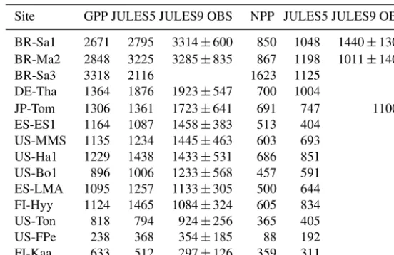
Table 5.Comparison of simulated and observed annual GPP and NPP at FLUXNET sites, listed in order from most to least productive. Units: g C m−2year−1. Results are color-coded so blue shows when there is an improvement. The GPP and NPP are based on similar data processing between the FLUXNET observations and model. Sources:1Malhi (2009);2Gower and Richards (1990), assuming 0.5 gC g−1 biomass.

Site GPP JULES5 JULES9 OBS NPP JULES5 JULES9 OBS

BR-Sa1 2671 2795 3314±600 850 1048 1440±1301 BR-Ma2 2848 3225 3285±835 867 1198 1011±1401

BR-Sa3 3318 2116 1623 1125

DE-Tha 1364 1876 1923±547 700 1004

JP-Tom 1306 1361 1723±641 691 747 11002

ES-ES1 1164 1087 1458±383 513 404

US-MMS 1135 1234 1445±463 603 693

US-Ha1 1229 1438 1433±531 686 851

US-Bo1 896 1006 1233±568 457 591

ES-LMA 1095 1257 1133±305 500 644

FI-Hyy 1124 1465 1084±324 605 834

US-Ton 818 794 924±256 365 405

US-FPe 238 368 354±185 88 192

FI-Kaa 633 512 297±126 359 311

span during a 30-year global simulation, where now JULES captures the observed leaf life spans.

Based on the new NA, Vcmax,25 was updated using the

new parameters iv andsv (Eq. 18; Fig. 2). The values

cal-culated from the TRY data are shown with asterisks, and these were used in the JULES9TRY experiments. The black

bars show the final Vcmax,25 after adjusting sv for the two

broadleaf evergreen tree PFTs and the needle-leaf decid-uous trees (see Sect. 2.3.3). Within the trees, the temper-ate broadleaf evergreen PFT has the highestVcmax,25, while

the needle-leaf deciduous and tropical broadleaf evergreen PFTs have the lowest. Because the JULES C3and C4PFTs

are assumed representative of natural vegetation, they have relatively low Vcmax,25 (compared to the range from K09

for C3). The NA calculated from median Nm and LMA

in this study (1.19 g N m−2) is lower than the average NA

reported in K09 (1.75 g N m−2). However, the C3Vcmax,25

(51.09 µmol CO2m−2s−1) is close to values reported

for European grasslands (41.9±6.9 µmol CO2m−2s−1and

48.6±3.5 µmol CO2m−2s−1 for graminoids and forbs,

re-spectively, in Wohlfahrt et al., 1999). In comparison to JULES5, the newVcmax,25is higher for all PFTs except for

C3 grass. Previously, the Vcmax,25 was lower than the

ob-served range for all non-tropical trees, but now theVcmax,25

for all PFTs is within the range of observed values. 4.2 Site-level simulations

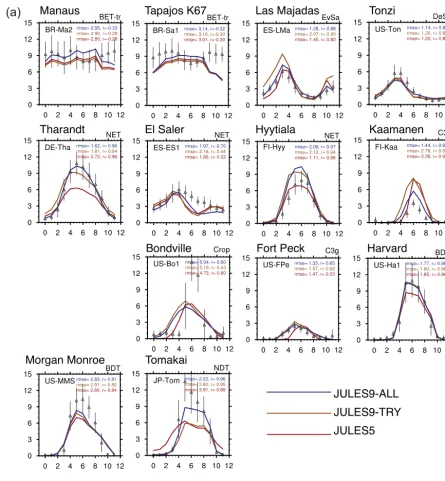
In most cases, the higher Vcmax from trait data increased

the GPP and NPP, and resulted in higher respiration fluxes due to both autotrophic (responding to higher GPP) and heterotrophic (responding to higher litterfall due to higher NPP) respiration. First, we compared JULES with five PFTs (JULES5) to JULES with nine PFTs and the TRY data

(JULES9TRY)(Experiments 1 and 2, respectively, in Table 3)

at the sites listed in Table 4. The results are summarized in Fig. 4, where yellows and reds indicate increased correlation (Fig. 4a, b) or reduced RMSE (Fig. 4c, d) in each experiment compared to JULES5. Using theNm, LMA, andVcmax,25data

from TRY improved the seasonal cycle of GPP at the two tropical forest sites, the evergreen savannah, and the crop site, and decreased the daily RMSE at one NET site (Tharandt), all grass sites, and the NDT site (Tomakai) (Experiment 1, Fig. 4). Enforcing the LMA–leaf life span relationship fur-ther improved the seasonal cycle at both savannah sites, the two natural C3 grass sites (the seasonal cycle was worse at

the crop site), and the NDT site, and further reduced RMSE at the deciduous savannah site and one BDT site (Harvard) (Experiment 2, a.k.a. JULES9TRY). In comparison, applying

all parameter changes summarized in Table 3 further reduced the RMSE at every site except the two tropical forests and further increasedrat every site except the tropical forests and the evergreen savannah (Experiment 7, a.k.a. JULES9ALL).

Overall, the carbon and energy exchanges were best cap-tured with JULES9ALL. Compared to JULES5, the RMSE

for GPP in JULES9ALLdecreased by more than 40 % at

Kaa-manen (C3 grass), Tharandt (NET), and Tomakai (NDT); the daily RMSE of NEE decreased at eight sites; andrincreased for NEE at 11 sites. The only sites without an improvement in either metric for NEE were Manaus (BET-Tr) and Bondville (Crop). The improvements to NEE were large at Tharandt (r from 0.61 to 0.76), Fort Peck C3grass (0.05 to 0.38), and

Tomakai (0.09 to 0.93), and RMSE for NEE decreased by more than 35 % at Kaamanen and Tomakai. Respiration and latent heat fluxes are discussed in the supplemental material. On an annual basis, GPP was higher in JULES9ALLthan

(12)

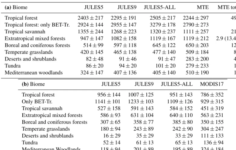
Table 6. (a)Area-weighted GPP from each biome (g C m−2year−1). The biome total GPP from MTE is given in Pg C year−1 to give perspective of each biome’s role in the global total.(b)Area-weighted NPP from each biome (g C m−2yr−1).

(a)Biome JULES5 JULES9 JULES5-ALL MTE MTE total

Tropical forest 2403±217 2295±191 2505±217 2244±297 49.9

Tropical forest: only BET-Tr. 2924±144 2955±147 3279±178 2790±273

Tropical savannah 1355±244 1268±223 1320±237 1111±257 21.9

Extratropical mixed forests 947±147 1082±158 1119±167 1119±212 2.9 (13.4*) Boreal and coniferous forests 514±99 597±118 645±122 650±203 12.1

Temperate grasslands 420±145 465±138 477±140 509±184 8.1

Deserts and shrublands 82±48 91±46 91±47 283±200 4.9

Tundra 86±20 94±20 101±20 279±233 1.9

Mediterranean woodlands 324±147 407±136 405±140 510±190 1.5

(b)Biome JULES5 JULES9 JULES5-ALL MODIS17

Tropical forest 956±144 1007±125 951±143 786±352

Only BET-Tr. 1141±101 1233±103 1109±126 929±315

Tropical savannah 527±158 591±143 584±152 451±319 Extratropical mixed forests 586±93 631±104 640±110 563±231 Boreal and coniferous forests 307±65 358±77 385±80 350±155 Temperate grasslands 180±94 243±89 242±90 304±247

Deserts and shrublands 16±29 35±29 33±29 111±133

Tundra 52±14 61±13 65±13 136±94

Mediterranean Woodlands 118±94 201±89 195±89 324±184

* Value for EMF (extra-tropical mixed forest) biome when agricultural mask is not applied.

El Saler (NET), Tonzi (savannah), and Kaamanen, and NPP was higher at every site except for Tapajós K77, El Saler, and Kaamanen (Table 5). Total GPP was improved at every site except for Hyytiälä (NET) and Las Majadas (savannah), where annual GPP was too high in JULES5, and at El Saler and Tonzi, where the modeled GPP was too low. However, for every site except Hyytiälä, JULES9ALL was within the

range of observed annual GPP. We now explore some site-specific aspects of the carbon cycle results.

4.2.1 Broadleaf forests

Both GPP and NPP were higher in JULES9ALLthan JULES5

for broadleaf forests due to a higher Topt of Vcmax and

a higher Vcmax,25. Simulated GPP was similar to

observa-tions in the absence of soil moisture stress. The increase in GPP occurred year-round at Manaus, but only during the wet season at Tapajós K67 (Fig. 5). GPP was similar in all JULES simulations during the dry season (October– December), when soil moisture deficits limited photosynthe-sis. The soil moisture stress factor,β, was<0.7 during these months, while it was >0.87 all year at Manaus (recall that a higher β indicates less stress). The reduction in GPP dur-ing the dry season at both sites is in contrast to the observa-tions, which show an increase from August–December. As a result, the simulated seasonal cycle of GPP was incorrect at both sites, and although the annual total GPP was closer to observations, the monthly RMSE was higher in JULES9ALL

compared to JULES5. The simulated NPP was too low in JULES5 at both sites. In JULES9ALL, the NPP was too high

at Manaus (by 187 g C m−2year−1)and too low at Tapajós (by 396 g C m−2year−1).

At the two BDT sites (Harvard and Morgan Monroe), the peak summer GPP was closer to observations in JULES9ALL.

GPP was very well reproduced at Harvard (BDT), where the average JJA temperature was 4◦C cooler than at Mor-gan Monroe (29◦C compared to 33◦C), and, due to differ-ences in the soil parameters, the soil moisture stress factor was higher (β >0.8 at Harvard compared to 0.5< β <0.7 at Morgan Monroe). At Morgan Monroe, the observed GPP was nearly zero from November–March, but all versions of JULES simulated uptake during November–December, when the average temperatures were still above freezing, possibly due to leaves staying on the trees for too long in the model. The RMSE of NEE decreased (Fig. 5b), but the amplitude of the seasonal cycle was too small at both BDT sites.

4.2.2 Needle-leaf forests

The seasonal cycle of GPP improved at the needle-leaf forests, but JULES9ALL underestimated GPP during

(13)

(a) GPP correlation (b) NEE correlation

(c) GPP RMSE (d) NEE RMSE

7: All 6: 2+structure

5: 2+A/Resp 4: 2+radiation 3: 2+gs

2: 1+LL 1: 9 PFTs + Nm,

LMA, Vcmax,25

7: All 6: 2+structure

5: 2+A/Resp 4: 2+radiation 3: 2+gs

2: 1+LL 1: 9 PFTs + Nm,

LMA, Vcmax,25

7: All

6: 2+structure 5: 2+A/Resp

4: 2+radiation 3: 2+gs 2: 1+LL

1: 9 PFTs + Nm,

LMA, Vcmax,25

7: All

6: 2+structure 5: 2+A/Resp

4: 2+radiation 3: 2+gs 2: 1+LL

1: 9 PFTs + Nm,

LMA, Vcmax,25

Figure 4.Relative changes in daily RMSE (Eq. 24) and monthly correlation coefficients (Eq. 25) for the JULES experiments in Table 4 compared to JULES5. Yellows and reds indicate an improvement in JULES compared to the FLUXNET observations.

months of June–October. During this period,β reduced to a minimum of 0.17 in August, and the GPP was too low by an average 1.83 g C m−2d−1. At all sites there was shift to-ward stronger net carbon uptake during the summer months with the new PFTs, which increased the correlation with ob-served NEE. At El Saler, the RMSE of NEE increased due to a change in the seasonal cycle of leaf dark respiration (Rd,

Eq. 8) resulting from the higherTopt. At Hyytiälä, the RMSE

of NEE increased due to higher rates of soil respiration dur-ing the winter months (Fig. S3; where soil respiration is the difference between total and autotrophic respiration).

Compared to JULES5 (with a needle-leaf PFT), both GPP and respiration were improved with the new NDT PFT at Tomakai, primarily due to an improved seasonal cycle of GPP with the deciduous phenology (Experiment 2). In JULES5, the LAI at the site was 6.0 m2m−2, compared to a summer maximum of∼3.5 m2m−2with the deciduous phe-nology and to a reported average LAI of larch of 3.8 m2m−2 (Gower and Richards, 1990). The new deciduous PFT also improved the seasonal cycle of NEE, and reduced errors in LE and SH (Fig. S4). The magnitude of maximum summer-time GPP was still underestimated, but this could be because the site is a plantation, where trees are evenly planted to op-timize the incoming radiation, rather than a natural larch for-est.

4.2.3 Grasses

GPP and NEE were improved for temperate grasslands (Kaa-manen and Fort Peck) and NEE was improved at a tropical pasture (Tapajós K77). Compared to JULES5, productivity in JULES9ALLwas higher at a temperate C3site (Fort Peck),

and lower at a cold C3site (Kaamanen) and the tropical C4

site. In terms of GPP, these changes brought JULES9ALL

closer to the observations (Table 5). With the new PFT pa-rameters, grasses had higher year-round LAI due to the re-moval of phenology, and GPP increased earlier in the year at Kaamanen, Bondville, and Fort Peck in JULES9ALL

com-pared to JULES5. Net uptake also occurred 1–2 months ear-lier in JULES9ALL(compared to JULES5), which decreased

RMSE and increasedrfor NEE at the three natural grassland sites. JULES9ALL underestimated productivity at Bondville

(crop site), but this is not surprising given that the PFT is meant to represent natural grasses. There is a separate crop model available for JULES (Osborne et al., 2015).

The Tapajós K77 pasture was not included in the set of sites with GPP/Reco partitioning. The simulated GPP was

lower in JULES9ALLthan in JULES5 due to the lower

quan-tum efficiency (Fig. S3c). The seasonal cycle of NEE was close to that observed during most months (Fig. 5b), and in terms ofrand RMSE JULES9ALLwere better than JULES5.

(14)

JULES9-ALL

JULES9-TRY

JULES5

Manaus

Tapajos K67

Las Majadas

Tonzi

Tharandt

El Saler

Hyytiala

Kaamanen

Bondville

Fort Peck

Harvard

Morgan Monroe

Tomakai

(a)

Figure 5.

GPP was higher at the forest site than at the pasture, and the NPP was similar.

4.2.4 Mixed vegetation sites

Las Majadas and Tonzi are savannah sites dominated by ev-ergreen and deciduous plants, respectively (assumed in the simulations to be an equal mix of trees, shrubs, and C3grass,

Table 4). Both GPP and NPP were better simulated with JULES9ALL at both sites, and the annual GPP was within

the range of the observations (although it was too high at Las Majadas and too low at Tonzi).

At Las Majadas, the GPP increased in JULES9ALL

(com-pared to JULES5) during the wet spring (January–April) due to high GPP from the BET-Te and C3grass PFTs. The former

had a higher year-round LAI (∼4.6 m2m−2),Vcmax,25, and

ToptforVcmaxcompared to the BT from the five PFTs (which

simulated maximum summer LAI of 3.8 m2m−2). For C3

grass, the newVcmax,25andToptwere lower in JULES9ALL,

but the removal of phenology (settingdT to 0) increased the

(15)

obser-JULES9-ALL

JULES9-TRY JULES5

Manaus Tapajos K67 Las Majadas Tonzi

Tharandt El Saler Hyytiala Kaamanen

Tapajos K77 Bondville Fort Peck Harvard

Morgan Monroe Tomakai

(b)

Figure 5. (a)Monthly mean fluxes of GPP. Observations±standard deviation from FLUXNET are shown with triangles and vertical lines. The three JULES simulations are JULES5 with standard five PFTs (JULES5, red); JULES with nine PFTs and new LMA,Nm, andVcmax,25 from TRY (JULES9TRY, orange); JULES9-TRY plus new parameters for the PFTs as discussed in Sect. 2.3 (JULES9ALL, blue). Also shown are the daily root mean square error (RMSE) based on daily fluxes and the correlation coefficient (r) based on monthly mean fluxes for all years of the simulations. Site information is given in Table 3. All units are in g C m−2d−1.(b)As in(a)but for monthly anomalies of NEE.

vations (r=0.70), but the April–May uptake was too strong and contributed to an overestimation of the annual GPP.

At Tonzi, GPP was similar to observations except during April–July, when it was too low. The modeled photosynthe-sis began to decline after March, coinciding with a rapid increase in simulated soil moisture stress and stomatal sistance. Moving from a generic to a deciduous shrub re-sulted in a large decrease in simulated GPP at this site. The shrub LAI decreased from∼3.3 m2m−2to a maximum of 1.5 m2m−2, and theVcmax,25for the DSh was slightly lower

than theVcmax,25for the generic shrub. Slightly

compensat-ing for the lower shrub GPP was a higher broadleaf tree GPP, with a higherVcmax,25andToptcompared to the previous

val-ues in JULES5. 4.3 Global results

(16)

JULES9-ALL

JULES5

Figure 6. Annual GPP and NPP for the eight biomes shown in Fig. 3b. Biome abbreviations are D – deserts, M – Mediterranean woodlands, TU – tundra, TG – temperate grasslands, TS – tropi-cal savannahs, BCF – boreal and coniferous forests, EMFs – extra-tropical mixed forests, TF – extra-tropical forests.

Fig. 3, and seasonal cycles are shown in Fig. 7. GPP in-creased in JULES9ALLcompared to JULES5 in all

extratrop-ical biomes, but it decreased in the two biomes with signifi-cant coverage by C4grass. For all biomes, the representation

of GPP in JULES9ALL was closer to the observed (MTE)

value. NPP increased in every biome, and this was an im-provement (relative to MOD17) in five biomes (boreal and coniferous forests, temperate grasslands, deserts/shrublands, tundra, and Mediterranean woodlands), but NPP was too high in tropical biomes and extratropical mixed forests.

In the tropical forests, the biome-averaged GPP and NPP increased in JULES9ALL compared to JULES5, and both

fluxes were∼200 g C m−2_yr−1_{higher than their respective}

observational value. The seasonality of rainfall in the trop-ics has a hemispheric dependence. Splitting the biome into the Northern and Southern hemispheres revealed that the seasonal cycle in Fig. 7a was most similar to the South-ern Hemisphere in terms of the climate and fluxes. In both hemispheres, the JULES GPP was higher than the MTE GPP during the transition period from the wet to the dry season and the early dry season. This is in contrast to the results at the two Brazilian FLUXNET sites, where JULES GPP was lower than that observed during the dry season.

Most of the differences between JULES5ALL and

JULES9ALLwere in the tropics (Fig. 9, Table 6). The global

GPP was relatively high (135 Pg C year−1) in JULES5ALL

(compared to 127 Pg C year−1 for JULES9ALL), primarily

becauseVcmaxfor the generic broadleaf tree was much higher

than for the tropical broadleaf evergreen PFT, based on the data from K09. Although tropical GPP was higher in JULES5ALL compared to JULES9ALL, the NPP in tropical

forests was lower and closer to the values from MODIS NPP. The reason was the differences in leaf nitrogen, which increased respiratory costs in JULES5ALL compared to

JULES9ALL. BothNAandNmwere higher for the broadleaf

tree PFT than for the tropical evergreen broadleaf tree PFT.

Over the tropical savannah biome, the GPP decreased in JULES9ALLcompared to JULES5 due to lower productivity

from C4grasses, and GPP was within the uncertainty range

of the MTE GPP, although slightly higher. The overestima-tion occurred during most of the year (Fig. 7b), except during the late dry season/early wet season (October–December). Although C4 grasses had a lower NPP in JULES9ALL, a

significant fraction of the biome is composed of C3 grass,

BDT, ESh, and DSh in the ESA data, which all had higher NPP in JULES9ALL. For this reason, biome-scale NPP was

higher in JULES9ALL than in JULES5, and simulated NPP

was 140 g C m−2year−1 higher than the MOD17 value. In the temperate grasslands biome, both GPP and NPP were higher in JULES9ALLcompared to JULES5, and closer to the

MTE and MOD17 values. However, compared to the MTE, the JULES9 GPP increased 1 month early, it was too low in the mid-summer, and it declined too slowly in the autumn.

The biome-scale GPP in the extratropical mixed forests improved in JULES9ALL compared to JULES5, and was

very close to the MTE estimate. The simulated GPP was overestimated during the autumn (September–October) and underestimated during the winter. Simulated NPP was very close to the MOD17 NPP in JULES5, but it is too high by∼100 g C m−2year−1 in JULES9ALL. The predominant

vegetation types in the “boreal and coniferous forests” biome are NET (26 % coverage), C3 grass (20 %), and

NDT (14 %). Shrubs, deciduous broadleaf trees, and bare soil cover the remaining 40 % of the biome. There was a large increase in summertime GPP in this biome, bringing JULES9ALLcloser to the MTE GPP than JULES5. The NPP

increased in JULES9, compared to JULES5, and was within 10 g C m−2_year−1_{of the MOD17 NPP.}

Deserts/shrublands and tundra are both dry environments with annual-average GPP of∼280 g C m−2year−1 accord-ing to the MTE data set. Although GPP increased in both biomes in JULES9ALL relative to JULES5, it was much

lower than the MTE value. In the tundra biome, GPP was underestimated during the entire growing season, and it was underestimated all year in the desert biome. The simulated NPP was also significantly lower than MOD17 in these two biomes, although it was slightly improved in JULES9ALL.

These results indicate that the JULES plants struggle in ex-tremely cold and arid environments.

In the Mediterranean woodlands, GPP increased by 90 g C m−2year−1and NPP increased by 80 g C m−2year−1 in JULES9ALL compared to JULES5, but both fluxes were

still ∼100 g C m−2_year−1 _{lower than the MTE GPP and}

MOD17 NPP. The simulated GPP (in JULES9ALL)was close

to the MTE value during most of the year except the dry sea-son, when it declined more in the model than in the MTE estimate.

On a global scale, JULES9ALL had a similar GPP but

(17)

Figure 7.Area-averaged seasonal cycles of GPP from the biomes shown in Fig. 3b, comparing JULES5, JULES9, and the Jung et al. (2011) MTE. Also shown are the temperature and precipitation from the CRU-NCEP data set used to force the JULES simulations. The gray shading in the GPP plots shows the MTE GPP±1 standard deviation based on the area-averaged standard deviations of monthly fluxes for each grid cell.

122±8 Pg C year−1. GPP was higher in JULES9ALL

com-pared to JULES5 in the core of the tropical forests, but lower in tropical/subtropical South America, Africa, and Asia. These are regions with significant grass coverage (Fig. 3a), especially C4 grasses. Poleward of 30◦, GPP was higher in

JULES9ALLdue to higher productivity in trees. In JULES5,

the global NPP (55 Pg C year−1)was close to the value from MODIS NPP (54 Pg C year−1). In JULES9ALL, the NPP was

higher than JULES5 almost everywhere (except for southern Brazil where C4grasses are dominant), and the global NPP

was 62 Pg C year−1.

5 Discussion

5.1 Impacts of trait-based parameters and new PFTs Including trait-based data on leaf N, Vcmax,25, and leaf life

span improved the seasonal cycle of GPP at seven sites,

es-pecially sites with C3grass and NDT. Parameterizing leaf life

span correctly has been shown to be important, even within biomes (Reich et al., 2014). Our study confirms this, as the simulation of GPP improved at fewer sites in the simulations without the improved leaf life span. However, compared to the standard five PFTs, the RMSE of GPP was only improved at four sites in JULES9TRY. Despite this, the new PFTs with

the new trait data include observed trade-offs between leaf structure and life span. These trade-offs are important for en-abling JULES to represent observed vegetation distribution and for predictions of future fluxes.

Incorporating more data and accounting for evergreen and deciduous habits further improved the model, as indicated by the closer model-data comparison obtained with JULES9ALL

(18)

Figure 8.Global maps of carbon cycle fluxes from 2000 to 2012. The observation sources are MTE (GPP) and MODIS MOD17 (NPP, 2000–2013).

seasonal cycle of NEE were improved at the warm-temperate evergreen savannah site (Las Majadas). This study has laid the groundwork for further improvements to JULES GPP and plant respiration by incorporating trait-based physiologi-cal relationships and allowing for a flexible number of PFTs. Future development can focus on more biome-specific data-model mismatches than was possible with the generic set of five PFTs.

The nine PFTs were chosen as they represent the range of deciduous and evergreen plant types with minimal exter-nally determined bioclimatic limits. The distinction between tropical and temperate broadleaf evergreen trees account for the important differences between these types of trees (e.g., a lowerVcmaxfor a givenNAin tropical broadleaf evergreen

trees: Kattge et al., 2009). The comparison of JULES5ALL

and JULES9ALLindicates that even using improved

parame-ters with five PFTs based on the TRY data and the literature reviewed in this study will give improved productivity fluxes in JULES. However, an important caveat is JULES was not run with dynamic vegetation for this analysis. The additional PFTs enable more diverse and specific dynamic responses to climate change.

5.2 Future development priorities

(19)

Figure 9.Differences between modeled and observed GPP (observed – MTE) and NPP (observed – MOD17).(a, b)JULES with the standard five PFTs and default parameters; (c, d)JULES with five PFTs and improved parameters;(e, f)JULES with nine PFTs and improved parameters.

A side effect of the trait-based parameters was increased respiration, and comparison to both FLUXNET sites and the MTE suggest it is now too high for most biomes. Total ecosystem respiration was higher than that observed at Man-aus, Harvard, Morgan Monroe, Tharandt, Hyytiälä, Kaama-nen, Las Majadas, and Tonzi (75 % of the sites with respira-tion data) (Fig. S3). As this study has focused primarily on improving the GPP, the next step should be to include a more mechanistic representation of growth and maintenance respi-ration in JULES to improve the net productivity (e.g., using data from Atkin et al., 2015). Comparison to the MTE res-piration also suggests that JULES soil resres-piration is too high during the winter in the temperate and boreal biomes. In the latter, both versions of JULES predicted positive respiration flux during the winter, while the MTE product showed negli-gible fluxes (Fig. S5). The average winter temperatures in the biome were<−13◦C, yet soil respiration continued during these months because theQ10soil respiration scheme has a

very slow decay of soil respiration flux at sub-zero tempera-tures (see Fig. 2 of Clark et al., 2011). A similar result was seen at Hyytiälä (Fig. S3b), which further indicates that win-tertime respiration might be too high.

Last, the simulation of GPP could be further improved by replacing the staticVcmax,25per PFT. Simultaneous with this

study, there is work to include temperature acclimation for photosynthesis JULES, which is more realistic than a setTopt

for each PFT. Also, the data exhibit large within-PFT varia-tion inVcmax,25(Fig. 2) and photosynthetic capacity can

de-pend on the time of year. Recent work relating photosynthetic capacity to climate variables, environmental factors, and soil conditions shows promise for better capturing the dynamic nature of this parameter (e.g., Verheijen et al., 2013; Ali et al., 2015; Maire et al., 2015).

6 Conclusions

We evaluated the impacts on GPP, NEE, and NPP of new plant functional types in JULES. All changes were evalu-ated in version 4.2 with the canopy radiation model 5 op-tion (Clark et al., 2011). At the base of the new PFTs was inclusion of new data from the TRY database.Nmand LMA

replaced the parametersNl0andσl. These were used to

cal-culate new Vcmax,25, which was higher for all of the new

PFTs compared to the original five, except for C3 grasses.

The higherVcmax,25resulted in higher GPP. The GPP did not

increase for C4grasses due to a lower quantum efficiency, or

(20)

Vcmax. Increases in NPP generally followed on from the

in-creases in GPP.

A trade-off between LMA and leaf life span was en-forced by changing parameters relating to leaf phenology, growth and senescence. The new parameter values changed the turnover rate of leaves on trees in the spring and fall, therefore altering the leaf life span in JULES in a manner consistent with observations. In JULES9TRY, the median leaf

life span of grasses and shrubs were reduced, which im-proved the seasonal cycle at the relevant sites (Las Majadas, Tonzi, Fort Peck, Kaamanen, and Tomakai). The exception was the Bondville crop site.

Including the full range of updated parameters (in JULES9ALL)resulted in an improved seasonal cycle of GPP

at 10 sites and reductions to daily RMSE at 11 sites (out of 13 sites with GPP data) compared to JULES9TRY. The annual

GPP was within the range of the FLUXNET observations at every site except for one (Hyytiälä). On a biome scale, we compared GPP to the MTE product of Jung et al. (2011) and NPP to the MODIS17 product. GPP was improved in JULES9 for all eight biomes evaluated, although for the tun-dra and desert/shrubland biome the GPP was much lower than the MTE value. The global NPP was slightly higher than that observed, but JULES9 was closer to MOD17 in most biomes – the exceptions being the tropical forests, sa-vannahs, and extratropical mixed forests where JULES9 was too high. The biome-averaged NPP from JULES9 was within the range of MOD17 NPP for all biomes.

Overall, the simulation of gross and net productivity was improved with the nine PFTs. The present study can be thought of as a “bottom-up” approach to improving JULES fluxes, with new parameters being based on large observa-tionally based data sets. The next step for improving PFTs in JULES is to evaluate the nine PFTs when the dynamic vege-tation is turned on. This will be addressed in a follow-up pa-per. A complimentary, “top-down” method for reducing un-certainty in JULES is to optimize PFT parameters based on minimizing errors between simulated and observed fluxes. This is currently being done with adJULES, an adjoint ver-sion of JULES (Raoult et al., 2016). Future model develop-ment within JULES will have more flexibility for improving the model with more PFTs, and the improvements presented in this study increase our confidence in using JULES in car-bon cycle studies.

7 Code availability

The simulations discussed in this manuscript were done us-ing JULES version 4.2. This can be accessed through the JULES FCM repository: https://code.metoffice.gov.uk/trac/ jules (registration required). For further details, see https: //code.metoffice.gove.uk/trac/jules/wiki/9PFTs. An example with the nine PFTs and parameters in this paper is provided for Loobos in the documentation directory of the JULES trunk. Summary tables of the traits LMA,Nm, and leaf life

(21)

Appendix A

Table A1.List of parameters and symbols in the text.

Symbol Units Equation Description Default

value∗

Al kg C m−2s−1 5 Leaf-level photosynthesis

a_wl kg C m−2 ₂₄ _{Allometric coefficient}

aws – 24 Ratio of total to respiring stem carbon

b_wl – 24 Allometric exponent 1.667

C_i Pa 6 Internal leaf CO₂concentration

Cmass kg C [kg biomass]−1 23 Leaf carbon concentration per unit mass 0.5 for this study

Cs Pa 6 Leaf surface CO2concentration

D_crit kg kg−1 7 Critical humidity deficit

dT – 16 Rate of change of leaf turnover with temperature

f₀ – 7 Stomatal conductance parameter

fd – 4 Leaf dark respiration coefficient

gs m s−1 6 Leaf-level stomatal conductance

iv µmol CO2m−2s−1 19 Intercept for relationship betweenNAandVcmax,25

kn – 3, 20 Extinction coefficient for nitrogen 0.78

h m 13, 23, 24 Canopy height

Lbal m2m−2 12, 13, 22–24 Balanced leaf area index (maximum LAI given the plant’s height)

Lmax m2m−2 _{Maximum LAI}

L_min m2m−2 Minimum LAI

LMA kg m−2 18, 21, 22 Leaf mass per unit area (new parameter)

Na kg N m−2 18 Leaf nitrogen per unit area

n_eff mol CO₂m−2s−1kg C [kg N]−1 3 Constant relating leaf nitrogen to Rubisco carboxylation capacity Nl0 kg N [kg C]−1 3 Top-leaf nitrogen concentration (old parameter, mass basis) Nm kg N kg−1 18, 21–23 Top-leaf nitrogen concentration (new parameter)

Nl kg N m−2 11, 21 Total leaf nitrogen concentration

Nr kg N m−2 12, 22 Total root nitrogen concentration

Ns kg N m−2 13, 23 Total stem nitrogen concentration

p – 17 Phenological state (LAI/L_bal)

Q_10,leaf – 2 Constant for exponential term in temperature function ofVcmax 2 Ra kg C m−2s−1 8 Total plant autotrophic respiration

R_d kg C m−2s−1 4, 5 Leaf dark respiration

rg – 10 Growth respiration coefficient 0.25

rootd m e-folding root depth

sv µmol CO2g N−1s−1 19 Slope betweenNAandVcmax,25

Tlow ◦C 1 Upper temperature parameter forVcmax

Toff ◦C 16 Threshold temperature for phenology

T_optb ◦C Optimal temperature forVcmax