www.geosci-model-dev.net/7/2803/2014/ doi:10.5194/gmd-7-2803-2014
© Author(s) 2014. CC Attribution 3.0 License.
The spectral element method (SEM) on variable-resolution grids:
evaluating grid sensitivity and resolution-aware
numerical viscosity
O. Guba1, M. A. Taylor2, P. A. Ullrich3, J. R. Overfelt2, and M. N. Levy4
1Department of Mathematics and Statistics, University of New Mexico, Albuquerque, New Mexico, USA 2Sandia National Laboratories, Albuquerque, New Mexico, USA
3Department of Land, Air and Water Resources, University of California Davis, Davis, California, USA 4National Center for Atmospheric Research, Boulder, Colorado, USA
Correspondence to: O. Guba ([email protected])
Received: 31 May 2014 – Published in Geosci. Model Dev. Discuss.: 25 June 2014 Revised: 8 October 2014 – Accepted: 21 October 2014 – Published: 27 November 2014
Abstract. We evaluate the performance of the Community Atmosphere Model’s (CAM) spectral element method on variable-resolution grids using the shallow-water equations in spherical geometry. We configure the method as it is used in CAM, with dissipation of grid scale variance, imple-mented using hyperviscosity. Hyperviscosity is highly scale selective and grid independent, but does require a resolution-dependent coefficient. For the spectral element method with variable-resolution grids and highly distorted elements, we obtain the best results if we introduce a tensor-based hy-perviscosity with tensor coefficients tied to the eigenvalues of the local element metric tensor. The tensor hyperviscos-ity is constructed so that, for regions of uniform resolution, it matches the traditional constant-coefficient hyperviscosity. With the tensor hyperviscosity, the large-scale solution is al-most completely unaffected by the presence of grid refine-ment. This later point is important for climate applications in which long term climatological averages can be imprinted by stationary inhomogeneities in the truncation error. We also evaluate the robustness of the approach with respect to grid quality by considering unstructured conforming quadrilateral grids generated with a well-known grid-generating toolkit and grids generated by SQuadGen, a new open source al-ternative which produces lower valence nodes.
1 Introduction
In climate and weather forecast applications, there is an in-creased demand for variable-resolution capabilities. This de-mand is motivated by the need to resolve various tempo-ral and spatial scales in forecast and regional climate stud-ies with limited computational resources. Several approaches can be employed to this end, including nesting techniques, multi-physics modeling, and multi-resolution simulations, recently overviewed in Ringler et al. (2011).
grids, and thus we consider two resolution-aware exten-sions. The first is the straightforward extension of allow-ing the hyperviscosity coefficient ν to depend on the local element length scale. This approach was used in Zarzycki et al. (2014a, b) for realistic CAM simulations. Here, we use the shallow-water equations to show some deficiencies with this approach and then that better results are obtained with a tensor-based hyperviscosity operator, which can bet-ter represent both length scales within non-square spectral elements. We evaluate this approach using the shallow-water equations on the sphere with the two-dimensional version of HOMME’s spectral element dynamical core. There have been other modifications of the viscosity and hyperviscos-ity operators. For example, Yu et al. (2014) uses a flow-dependent coefficient for the Laplacian. In Dobrev et al. (2012), several tensor coefficient viscosity operators were considered, including a formulation in which directional vis-cosity coefficients were chosen to depend on directional length scales of a deformed Lagrangian volume. Here, we follow a similar approach, but the length scales come from the deformation of the elements, especially those in the grid transition region.
The mimetic SEM requires conforming quadrilateral grids. To generate variable-resolution grids, we employ a well-known grid-generating toolkit, CUBIT (https://cubit. sandia.gov). In the grid-transition region, the CUBIT grids have many valence 6 nodes (corner nodes shared by six ele-ments). For grids in spherical geometry, it is possible to con-struct transition regions with mostly valence 5 nodes, and such elements will have less acute angles. To generate grids with low-valence nodes, we use the Spherical Quadrilat-eral Grid Generator (SQuadGen, http://climate.ucdavis.edu/ squadgen.php). This toolkit uses a paving technique (Blacker and Stephenson, 1991) in combination with a set of low-valence tiles to generate smooth quadrilateral grids based on cubed-sphere geometry. Regions of enhancement are de-termined via a user-specified image file, which is mapped onto a cubed-sphere grid. Grid smoothing is performed via straightforward application of spring dynamics in three-dimensional geometry (Persson and Strang, 2004). Grids ob-tained via this technique exhibit several improved character-istics, including greater uniformity in the transition region, and elements with angles that are closer to 90◦.
In this study, we use multi-resolution grids with a sin-gle region of quasi-uniform high resolution (1xhigh), which transitions to a quasi-uniform grid of low resolution (1xlow), covering most of the globe.
While evaluating the model’s performance, it is natural to compare the multi-resolution simulation with the corre-sponding 1xlow and1xhigh uniform grid simulations. Mo-tivated by climate applications, and following Weller et al. (2009); Ringler et al. (2011), we evaluate 1xlow/1xhigh variable-resolution simulations with two criteria:
1. Refinement does no harm to the global scales. For the shallow-water equation initial value problem, at short times, it is reasonable to expect many features in the re-fined region would not be contaminated by information from the low-resolution region. In contrast, for longer times, we expect all features to be influenced by infor-mation from both the low- and high-resolution regions. So, in general, global errors should depend on1xlow and may not be improved by the presence of a1xhigh resolution region. However, they should not be wors-ened by the presence of refinement and we thus expect global errors in a multi-resolution simulation to be as low as those obtained by a uniform1xlowsimulation. 2. Local scales are resolved in the refined region. The
pur-pose of the multi-resolution approach in climate mod-eling is not to reduce the initial value problem error, but to resolve features of interest, such as hurricanes, eddies, or topographically driven features in select gions at a lower cost. We thus expect that, in the re-fined region, the multi-resolution simulation can resolve the same scales as the uniform1xhighresolution simu-lation. With hyperviscosity, this requires a resolution-aware formulation, which locally matches what would be used in a uniform resolution simulation.
In the study, we use the popular set of shallow-water test cases on the sphere compiled by Williamson et al. (1992) to show that the SEM satisfies both requirements when tensor hyperviscosity is used. We show that tensor hyperviscosity is both more accurate and more robust with respect to grid qual-ity. The rest of the paper is organized as follows: in Sect. 2, we introduce two dissipation mechanisms – scalar and tensor hyperviscosity; in Sect. 3, we discuss grid refinement tech-niques; in Sect. 4, we describe shallow-water test cases; in Sect. 5, we present numerical results.
2 Hyperviscosity formulations
In many climate models, a hyperviscosity term is added to the right hand side of the dynamical equations for both phys-ical and numerphys-ical reasons. Hyperviscosity is preferred over regular viscosity because it is more scale selective. It strongly damps grid scale modes while having less of an impact on the resolved large-scale modes. To introduce the various types of hyperviscosity that will be considered here, we first consider a model equation containing only the hyperviscosity opera-tor:
Qt = −ν12Q, ν >0, (1)
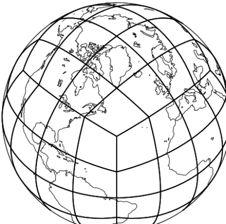
Figure 1. A cubed-sphere grid.
consider
Qt= −(∇ ·τ∇)1Q. (2)
Our intention is to derive a formulation forτ that is suit-able for uniform and quasi-uniform grids and that can be ex-tended to non-uniform grids.
We start by writing equation Eq. (2) in weak form. Since Eq. (2) is equivalent to the set of equationsQt= −(∇ ·τ∇)q, q=1Q, we rewrite the set as a system of integral equations:
Z
φ1Qt= Z
∇φ1·τ∇q, (3)
Z
φ2q= − Z
∇φ2· ∇Q. (4)
Here,is the problem domain, which, in our case, will be the sphere of the radius R. This system of equations is discretized by the standard SEM and solved for all SEM test functionsφ1andφ2. We first decompose the domaininto a set of quadrilateral elements on the surface of the sphere (m,m=1, . . ., M, as in Fig. 1), and then write
X
m Z
m φ1Qt=
X
m Z
m
∇φ1·τ∇q, (5)
X
m Z
m
φ2q= − X
m Z
m
∇φ2· ∇Q. (6)
Each term in this sum is then written as an integral over the reference element ref= [−1,1] × [−1,1]. We define
r(x;m)as the map fromreftom, withr∈mas a point
on the sphere andx=(x1, x2)∈ref. We require this map to be differentiable and invertible, and further define
D=∂r/∂x, (7)
where D is a 2×2 matrix whose columns are the covariant basis vectors expressed in spherical coordinates. The map and analytic expressions for D are given in the Appendix. The integral over each spherical element m can then be
written with respect to ref, using derivatives with respect to the reference element coordinates:
Z
m
∇φ·τ∇q
=
Z
ref
∂φ ∂x1
∂φ ∂x2
!T
D−1τD−T
∂q ∂x1
∂q ∂x2
!
det(D)dx1dx2, (8)
where det(D)dx1dx2is the transformed area measure, andτ is the tensor expressed in spherical coordinates.
Note that the discrete operator will conserve mass (R Q), since the change in mass is obtained by taking test function
φ1=1, and then the right hand side of Eq. (5) will be 0 if we ensure∇1=0.
We now consider the eigenvalues of the metric tensor and its inverse:
DTD=E
λ1 0
0 λ2
ET,D−1D−T=E
λ−11 0 0 λ−21
ET, (9)
with the orthonormal matrix E whose columns are the ba-sis vectors, which diagonalize the Laplace operator. For any practical grid, both D and D−1are well defined, and hence the symmetric metric tensor is guaranteed to have such an eigenvalue decomposition with positive eigenvalues. We note that these two eigenvalues can be used to define the two length scales associated with each elementm. For the
spe-cial case of a grid of rectangular elements in Cartesian geom-etry of sizelx×ly, we have E as the identity matrix and λ1=(lx/2)2λ2= ly/2
2
. (10)
For a general, possibly distorted element, we define its two length scales by 2√λ1and 2
√
λ2.
2.1 Constant-coefficient hyperviscosity
et al., 2012). We take a slightly more general form and al-low ν=c0(1x)s for a scaling parameter s. The constant-coefficient hyperviscosity is used for quasi-uniform grids, where we follow the convention of defining1x by the aver-age number of degrees of freedom on the equator. For square elements,lx=p1x, wherepis the polynomial order of the
basis functions in the SEM.
In order to motivate how we generalize this operator to a full tensor, we first expressτ=νI in the basis, which diag-onalizes the Laplace operator (the local element basis defined by E). Some algebra shows that
E−1D−1τD−TE−T =
νλ−11 0 0 νλ−21
.
Below, we ensure that the more general tensor formula-tions retain this scaling in regions in which the grid has a uniform resolution ofλ1'λ2.
2.2 Scalar hyperviscosity
For scalar hyperviscosity, we once again take τ=νI and now allow ν to vary in space. The natural choice is to use the same scaling as with the constant-coefficient operator,
ν=c0(1x)s, but with1x now chosen locally for each el-ement. To preserve the scaling for the constant-coefficient operator, but also to ensure that the coefficient does not be-come too small (and thus provide insufficient dissipation), we use Eq. (10) and approximate the resolution locally by taking
lx=2(max{λ1, λ2})1/2and1x=lx/p. For scalar
hypervis-cosity, this tensor scales according to E−1D−1τD−TE−T =
νλ−11 0 0 νλ−21
, ν=c0(1x)s.
On a Cartesian grid with square elements, λ1=λ2= (lx/2)2, and so the scalar and constant-coefficient
opera-tors are identical. For a quasi-uniform grid, whereλ1'λ2' (lx/2)2, the scalar and constant-coefficient operators will
have the same scaling with resolution. 2.3 Tensor hyperviscosity
Now consider a grid with only rectangles of size lxly.
Based on our expected scaling hyperviscosity with resolu-tion, we note that the scalar hyperviscosity above would give us the desired amount of dissipation in the x direction, but would have excessive dissipation acting in the y direction. The natural choice for a grid of rectangles is a tensor coeffi-cient:
τ =
ν1 0
0 ν2
ν1=c0(1x)s, ν2=c0(1y)s. (11) For a grid of pure rectangles, D is diagonal and E=I, so τ expressed in the E basis is given by
E−1D−1τD−TE−T =
ν1λ−11 0 0 ν2λ−21
. (12)
We use this same formulation for unstructured grids by defining the two locally varying element length scales as in Eq. (10) and taking ν1=c0(2
√
λ1/p)s and ν2= c0(2
√
λ2/p)s. On a Cartesian grid of pure rectangles, the scalar and tensor operators are identical. For a quasi-uniform grid of rectangles, whereλ1'(lx/2)2andλ2'(ly/2)2, the
scalar and tensor operators will have the same scaling with resolution.
For direct comparison, we summarize the three different approaches:
– Constant-coefficient: for quasi-uniform grids with aver-age grid spacing1x;
τ=νI=DE
νλ−11 0 0 νλ−21
(DE)T ν=c0(1x)s.
– Scalar: ν=ν(r) depends on local element length scales;
τ=νI=DE
νλ−11 0 0 νλ−21
(DE)T ν=c0(1x)s
1x=2pmax{λ1, λ2}/p.
– Tensor:τ depends on local element length scales; τ=DE
ν1λ−11 0 0 ν2λ−21
(DE)T ν1=c0(1x)s,
1x=2pλ1/p ν2=c0(1y)s,
1y=2pλ2/p.
For a smoothly deformed grid, the matrix entries ofτ will be smooth functions over the domainm. For our discrete
grids, we ensureτis continuous across element edges by ap-plying the standard SEM projecting operation to each entry ofτ. We further reduce variations inτby computing it only at element corner points, forming a bilinear fit to these cor-ner values, and using this bilinear approximation at all nodes within the element.
2.4 Hyperviscosity acting on vector fields
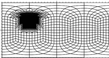
Figure 2. Schematic idea of constructing refined grids for the
con-formation of quadrilaterals on a sphere: we start from uniform grid with 1xlow. Next, the region of desired refinement is replaced
with uniform elements of size1xhigh. The grey area approximately
defines a transition region, which is constructed by substituting quadrilaterals with 1xlow by transition templates. After the
tran-sition region is assembled, spring dynamics can be used to smooth the grid.
3 High- and low-connectivity conforming quadrilateral grids on the sphere
The mimetic formulation of the SEM that we are using re-quires the conformation of quadrilateral grids. The cubed sphere is a popular way to construct these grids on the sphere with quasi-uniform resolution. An inscribed cube is pro-jected onto the surface of the sphere and each panel is further subdivided into a grid of elements, as shown in Fig. 1.
For multi-resolution, we consider grids with a single re-fined region over an area of interest. We define a coarse reso-lution1xlowand fine resolution1xhigh. We restrict ourselves to choices1xhigh=1xlow/N,N=2,4 and 8. Starting from a cubed-sphere grid with a resolution of 1xlow, the region under refinement is substituted by uniform elements with
1xhigh, as shown in Fig. 2. The approximate placement of the transition region is colored grey. For each N, we gen-erate a family of grids with different low-resolution regions (1xlow). Following Ringler et al. (2011), we refer to these family of grids as×1,×2,×4, and×8. The×1 family is the set of uniform cubed-sphere grids, with resolutions ranging from 3 to 0.5◦. The×2 family (shown in Fig. 3) is similar, but each×2 grid has a refined region with twice the resolu-tion (N=2). The×4 family has a refined region with four times the resolution (N=4) and the×8 family hasN=8.
It is nontrivial to construct the transition region. We need to avoid hanging nodes and prefer the elements to be as close to squares as possible. In Fig. 4, we provide two example
×8 grids with the same1xlow=3◦. Here, we represent two approaches to construct the transition region. Both are based on periodic templates, as seen in Fig. 5. The transition region in Fig. 5a is constructed by CUBIT, a grid-generating soft-ware for complex geometries in two and three dimensions (https://cubit.sandia.gov). Figure 5b contains the transition
(a) xlow= 3
(b) xlow= 1.5
(c) xlow= 0.75
Figure 3. A family of×2 grids with (from left to right)1xlow=3,
1.5, and 0.75◦,1xhigh=1xlow/2.
generated by SQuadGen. SQuadGen was developed to gener-ate two-dimensional refined spherical grids based on a cubed sphere (http://climate.ucdavis.edu/squadgen.php).
As seen in Fig. 5, the transition region in Fig. 5a contains nodes of higher valence comparing to the similar region in Fig. 5b. In this context, valence of a node is a number of edges to which it is connected. Node valence greater than 4 results in quadrilaterals with more acute angles and more distorted elements, and thus lower valence grids are usually preferred. In Fig. 5a, most nodes are of valence 3–6, with a few of valence 7. In Fig. 5b, most nodes are of valence 3–5 with a few nodes of valence 6. For the approach used in Fig. 5a, it is possible to avoid valence-7 nodes altogether with a less automated, more user-dependent procedure, but it is not possible with valence-6 nodes.
Pers-(a) Grid with a narrow, more distorted transition region from CUBIT mesh generation software with grid smoothing turned off
(b) Grid with a wider, more uniform transition region from SQuadGen and grid smoothing with spring dynamics
Figure 4. Example of ×8 refined grids with 1xlow=3◦ and 1xhigh=1xlow/8.
son and Strang (2004) with a uniform spring force function. Moreover, the user can choose a halo size around the in-ner and outer boundaries of the transition region, in terms of graph distances. This halo is then used to define a region in which smoothing will be applied. To investigate the per-formance of our resolution-aware hyperviscosity operators, we take two extremes: non-smooth grids with higher valence nodes generated by CUBIT, and smoothed grids with lower valence nodes generated by SQuadGen. We call the former high-connectivity (or highly distorted) grids and latter low-connectivity grids.
4 Shallow-water test cases
The shallow-water equations on a rotating sphere are given by
∂u
∂t +(ζ+f )k×u+ ∇
1
2u
2+g(h+b)
= −∇ ·τ∇1u (13)
∂h
∂t + ∇ ·(hu)= −∇ ·τ∇1h. (14)
Here,h is the fluid thickness,urepresents velocity, ζ=
k· ∇ ×u the vorticity, f is the Coriolis parameter, g is
(a) CUBIT approach (b) SQuadGen approach
Figure 5. Different types of refined conforming quadrilateral grids.
Plots (a) and (b) show close-ups of the transition regions from plots in Figs. 4a and b, respectively.
gravity, and b denotes bottom topography. The equations are discretized following Taylor and Fournier (2010) with the hyperviscosity operator discretized, as per Sect. 2. We takep=3 for a fourth-order accurate spatial discretization and use the second-order accurate leapfrog–trapezoidal time-stepping method.
For our studies, we choose two standard shallow-water test cases from Williamson et al. (1992): test case 2 (TC2) and test case 5 (TC5). TC2 represents a global steady state zonal geostrophic flow. Since the analytical solution is known, TC2 is often used to investigate convergence rates. The solution is very smooth, resulting in small errors, but the errors are very sensitive to local fluctuations in truncation error, such as those caused by grid irregularities. Following Ringler et al. (2011), we run TC2 for 12 simulation days, instead of the originally proposed 5 days, in order to allow longer time for the error growth to disrupt the steady state solution.
TC5 consists of a more realistic zonal flow over an isolated mountain run for 15 days. Error measures are obtained from a high-resolution reference simulation. Establishing conver-gence rates is difficult as the rate decreases to 0 as the errors approach the uncertainty in the reference solution. Instead, global errors are used primarily to measure the impact of the refined region. TC5 has much larger errors than those in TC2, which are less sensitive to small fluctuations in the lo-cal truncation error. In TC5, we examine the vorticity, which contains small-scale structures that are only captured at high resolution. We use the vorticity results to ensure that these structures can also be captured within the high-resolution re-gion of a variable-resolution grid.
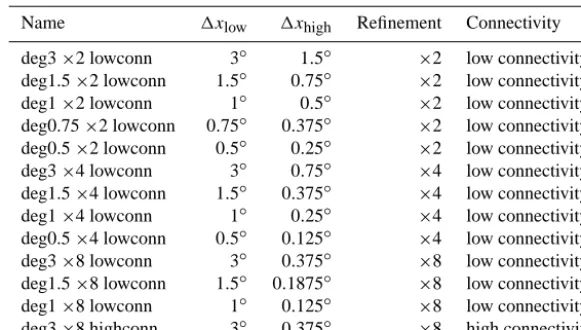
charac-Table 1. Summary of the×2,×4, and×8 family of grids.
Name 1xlow 1xhigh Refinement Connectivity
deg3×2 lowconn 3◦ 1.5◦ ×2 low connectivity deg1.5×2 lowconn 1.5◦ 0.75◦ ×2 low connectivity deg1×2 lowconn 1◦ 0.5◦ ×2 low connectivity deg0.75×2 lowconn 0.75◦ 0.375◦ ×2 low connectivity deg0.5×2 lowconn 0.5◦ 0.25◦ ×2 low connectivity deg3×4 lowconn 3◦ 0.75◦ ×4 low connectivity deg1.5×4 lowconn 1.5◦ 0.375◦ ×4 low connectivity deg1×4 lowconn 1◦ 0.25◦ ×4 low connectivity deg0.5×4 lowconn 0.5◦ 0.125◦ ×4 low connectivity deg3×8 lowconn 3◦ 0.375◦ ×8 low connectivity deg1.5×8 lowconn 1.5◦ 0.1875◦ ×8 low connectivity deg1×8 lowconn 1◦ 0.125◦ ×8 low connectivity deg3×8 highconn 3◦ 0.375◦ ×8 high connectivity
Table 2. Summary for simulations. TC stands for a test case, and the numbers inc0andsare parameters in the hyperviscosity coefficient ν=c0(1x)s.
TC Grid HV method c0 s 1t Figure
TC2 uniform, 3◦ constant coef. 6.12×10⁻⁶ 4 50 s Fig. 6a TC2 deg3×8 highconn scalar 6.52×10⁻⁶ 4 30 s Fig. 6b TC2 deg3×8 highconn tensor-based 6.12×10⁻⁶ 4 30 s Fig. 6c TC2 deg3×8 lowconn scalar 6.52×10⁻⁶ 4 30 s Fig. 6d TC2 deg3×8 lowconn tensor-based 6.12×10⁻⁶ 4 30 s Fig. 6e TC5 uniform, 3◦ constant coef. 7.18×10⁻² 3.2 50 s Fig. 10a TC5 deg3×8 highconn scalar 7.18×10⁻² 3.2 20 s Figs. 9b, 10b TC5 deg3×8 lowconn tensor-based 3.59×10⁻² 3.2 50 s Figs. 9c, 10c TC5 deg3×8 highconn tensor-based 3.59×10⁻² 3.2 50 s Fig. 10d
teristics of the grids in Table 1. In Table 2, we summarize some parameters for simulations in Figs. 6–10. Resolutions
1xlowand1xhighare computed according to the formula for an equatorial uniform resolution, considering that the whole sphere is covered by corresponding large or small elements.
5 Numerical results
5.1 Grid and hyperviscosity sensitivity in TC2
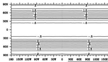
We present error plots for the TC2 height fieldhafter 12 days in Fig. 6. The error
1h=hnumerical−hanalytic (15)
is contoured for several different meshes all with a rela-tively low1xlow=3◦resolution. Part a contains a plot for a uniform resolution and constant-coefficient hyperviscosity. Plots b and d are simulations with the scalar hyperviscosity on ×8 grids. Plots c and e are simulations with the tensor hyperviscosity on×8 grids.
We first note that the errors are quite small relative to the height field (which ranges from 1000 to 3000 m). The height
field is not plotted since it would be identical to the analytic solution in Williamson et al. (1992). For the uniform grid with constant-coefficient hyperviscosity, the error is quite uniform with no indication of any grid sensitivity. There is no visiblem=4 mode that might be expected because of the cubed-sphere grid.
(a) Error plot for the uniform grid. The resolution is xunit=
3. The error varies from 6.06⇥10 1to2.02
⇥100.
(b) Scalar hyperviscosity with the highly distorted⇥8 grid shown in Fig. 4(a), error varies from 2.61⇥100to5.44
⇥100meters
(c) Tensor hyperviscosity with the highly distorted ⇥8 grid shown in Fig. 4(a), error varies from 5.32⇥10 1to1.90
⇥100
meters
(d) Scalar hyperviscosity with the low-connectivity ⇥8 grid shown in Fig. 4(b), error varies from 3.09⇥100to7.73
⇥100
meters
(e) Tensor hyperviscosity with the low-connectivity⇥8 grid shown in Fig. 4(b), error varies from 4.85⇥10 1to1.91
⇥100
meters
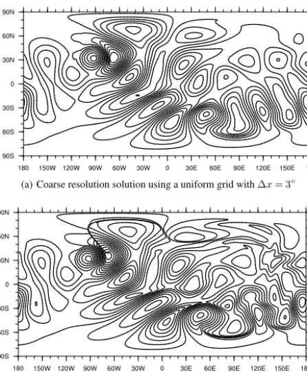
Figure 6. Error plots for TC2. A contour spacing of 0.25 m is the same for all plots. Maximum and minimum values of error Eq. (15) are given in captions. Tensor hyperviscosity produces smoother fields comparing to scalar hyperviscosity, as follows from comparing pairs (b),
(c), (d), and (e). In addition, the quality of the underlying grid significantly improves the outcome around the refined region when using
scalar hyperviscosity, as seen by comparing (b) and (d). Contrary to scalar hyperviscosity, tensor hyperviscosity is more robust with respect to mesh quality, as follows from comparing (c) and (e). Simulations (c) and (e) with tensor hyperviscosity also exhibit a substantial error reduction in the vicinity of the refinement compared to the coarse uniform resolution in (a).
zonal contours similar to panel a and somewhat less noise in the refined mesh region, although panel d does have larger minimum and maximum errors (given in the figure caption) than panel b. Both panels b and d have minimum and maxi-mum errors significantly larger than those in panel a.
Contrary to this, results using the tensor coefficient hyper-viscosity are very close to panel a and much less sensitive to the different types of refinement. The minimum and maxi-mum errors with either the distorted grid (panel c) or the low-connectivity grid (panel e) are slightly less than the values obtained on the uniform grid (panel a). In both panels c and e, the error contours in the Southern Hemisphere are almost identical to panel a. In the Northern Hemisphere, the errors
are sensitive to the presence of refinement, but are actually lower in this region than they are with panel a. Thus, with the tensor hyperviscosity, the presence of mesh refinement does no harm to the solution and actually results in a minor local reduction in the error.
5.2 Vorticity in TC5
(a) Coarse resolution solution using a uniform grid with x= 3
(b) High resolution reference solution, using a uniform grid with x= 0.125
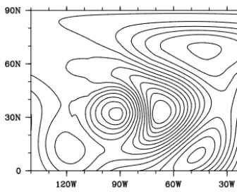
Figure 7. TC5 vorticity contours for low and high uniform
resolu-tions with constant-coefficient hyperviscosity. The contour spacing is 5.0×10⁻⁶s−1. A spherical mountain approximately 30◦in di-ameter is centered at 30◦N and 90◦W.
high-resolution grid. Note the sharp gradient in the flow that is well resolved in our reference solution but not present in the low-resolution result.
We show results computed using locally refined grids in Figs. 9 and 10. Based on the results presented for TC2, here we compare the worst and best performing extremes: scalar hyperviscosity running on the highly distorted ×8 mesh in Fig. 4a, and tensor hyperviscosity on the low-connectivity
×8 mesh in Fig. 4b.
The vorticity is plotted over the mesh refinement region for these two simulations in Fig. 9. The computation with scalar hyperviscosity develops unphysical oscillations, which are not present in the tensor hyperviscosity result or reference so-lution. Figure 9b shows a very smooth field across the highly non-uniform transition region, and the sharp gradient that is present in Fig. 8b is resolved without numerical noise. Note that the exact matching of Figs. 8b and 9b is not expected because the reference solution used a grid with 3 times finer resolution than the finest resolution used in the×8 grids.
To quantify these observations, we plot the error in the vorticity
1ζ=ζnumerical−ζreference (16)
field in Fig. 10. We show the error for the two×8 simula-tions, as well as a uniform low-resolution simulation. The er-ror is computed using our high-resolution reference solution as an approximation to the exact solution. The noise seen in the scalar hyperviscosity vorticity field (Fig. 9) is more evi-dent throughout the refined region in the vorticity error plot (Fig. 10b). With the tensor viscosity on the low-connectivity grid, Fig. 10c shows very little noise in the refinement re-gion and the mesh transition rere-gion. In addition, the error is substantially reduced in the refinement region as compared to the low-resolution uniform grid solution (Fig. 10b). The fact that the error can be reduced by local mesh refinement after 15 days in this region suggests that the solution con-tains standing features induced by the mountain, which ben-efit from mesh refinement and are not sensitive to the solu-tion in the rest of the domain in which both grids have the same1xlow resolution. In fact, the improved resolution of these standing features leads to slightly less errors than are obtained by the global1xlowresolution grid.
To investigate effects of tensor hyperviscosity, one can compare panels Fig. 10b (scalar hyperviscosity and the highly distorted grid) and Fig. 10d (tensor hyperviscosity and the highly distorted grid). The numerical noise in the transi-tion region present in the simulatransi-tion with scalar hypervis-cosity is practically eliminated when tensor formulation is used. If the simulation in Fig. 10c with a better-quality grid (low-connectivity grid) is considered optimal, then one can conclude that the tensor hyperviscosity simulation provides a very close-to-optimal result, even if a low-quality grid is used.
5.3 Convergence under grid refinement
We now present mesh convergence results for several choices of local refinement. We use our best configuration: tensor hy-perviscosity running with low-connectivity grids. We com-pare the convergence properties of the method with uni-form grids using constant-coefficient hyperviscosity, uniuni-form grids using tensor coefficient hyperviscosity, the×2 family of grids, the×4 family of grids, and the×8 family of grids. The×2,×4, and×8 simulations all use tensor hyperviscos-ity.
(a) Coarse resolution solution with x= 3. (b) High resolution reference solution, using a uniform grid with
x= 0.125.
Figure 8. As in Fig. 7 but plotted in a subregion of the global domain.
(a) Scalar hyperviscosity with the highly distorted⇥8 grid shown in Fig. 4(a).
(b) Tensor hyperviscosity with the low connectivity ⇥8 grid shown in Fig. 4(b).
(c) The highly distorted grid used in (a) (d) The low connectivity grid used in (b)
Figure 9. Contour plots of TC5 vorticity are shown in the top panels, while the grid is shown in the bottom panel. The contour interval
is 5.0×10⁻⁶s−1. All panels show a subregion of the global domain, which contains most of the refined region and is identical to the subregion used in Fig. 8. Panel (a) shows results using scalar hyperviscosity on the highly distorted grid shown in (c). Panel (b) shows results using tensor hyperviscosity on the low-connectivity grid shown in (d). The improved hyperviscosity and mesh quality result in significantly improved results.
the time is1t. For the refined grid with spatial scales1x/2, we execute a simulation with1t /4.
The globall2 errors for the TC2 height field for all these families of grids are shown in Fig. 11. We use the relative
l2, defined in Williamson et al. (1992). As noted in Sect. 2.1, the hyperviscosity scaling with resolution is typically cho-sen ass=3.2. For TC2, we instead chooses=4, so that the hyperviscosity term goes to 0 at a fourth-order rate and we
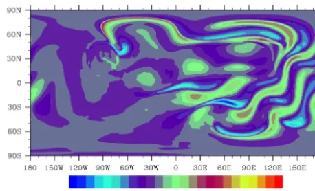
Figure 10. The error in the TC5 vorticity field is plotted for the global domain. The color scheme given in (a) is the same for all plots. The
tensor hyperviscosity again produces the best results with very little noise. From comparing panel (c) (tensor hyperviscosity and the low-connectivity grid) and panel (d) (tensor hyperviscosity and the highly distorted grid), we conclude that tensor hyperviscosity is not sensitive to grid quality.
fourth-order convergence, with the tensor and scalar hyper-viscosity results being nearly identical. Similar results are obtained for the ×2, ×4, and ×8 family of grids. The er-ror is completely determined by1xlowfor all grids, and all grids show fourth-order convergence under mesh refinement
with respect to 1xlow. Thus, the presence of mesh refine-ment, with refinements as much as 8×, does no harm to the global errors.
3 1.5 1 0.75 0.5 10−7
10−6 10−5 10−4 10−3
coarse−region grid spacing in degrees 4th order slope
Uniform resolution, tensor hyperviscosity Refinement x2
Refinement x4 Refinement x8
Uniform resolution, constant−coef hyperviscosity
Figure 11. TC2l2errors for uniform and low-connectivity grids
plotted as a function of1xlow. The solid line shows fourth-order
convergence. The error is controlled by the coarse region 1xlow
and the SEM obtains its formal order of accuracy (fourth order for p=3) with respect to1xlow. This is true for both uniform
grids (blue squares and blue stars) and grids containing mesh re-fined regions with1xhigh=1xlow/2 (×2 family, shown as red
di-amonds),1xhigh=1xlow/4 (×4 family, shown as red plus marks),
and 1xhigh=1xlow/8 (×8 family, shown as black squares). All
curves are practically indistinguishable.
function of 1xlow and normalized as in Williamson et al. (1992). For TC5, we return to the conventional hypervis-cosity resolution scaling of s=3.2. For TC5, we compute thel2errors from our high-resolution reference solution. The convergence rates are lower in this case due to the fact that the mountain is not smooth, limiting the convergence to the first order in the max norm and second order in thel2norm. We first note that, for uniform resolution grids, the constant-coefficient hyperviscosity performs nearly identically to the tensor coefficient hyperviscosity. For TC5, we also see that, for grids with the same1xlow, the globall2error is slightly reduced by the presence of mesh refinement, as conjectured in Sect. 5.2. The effect is small and fully captured by the×2 grid with twice the resolution over the TC5 mountain. Fur-ther local refinement in the×4 and×8 grids does not further improve the error. Thus, in this case, the presence of mesh refinement does no harm to the global errors and, in some special cases, can decrease global error.
6 Conclusions
We compared two resolution-aware hyperviscosity operators for the SEM running on unstructured grids with a region of local mesh refinement: a conventional scalar approach based on a single length scale for each element, and a tensor ap-proach that respects the resolution scaling of both length scales within each element. In both shallow-water test case
3 2 1.5 1 0.75 0.5
10−6 10−5 10−4 10−3 10−2
coarse−region grid spacing in degrees 3rd order slope
Uniform resolution, tensor hyperviscosity Refinement x2
Refinement x4 Refinement x8
Uniform resolution, constant−coef hyperviscosity
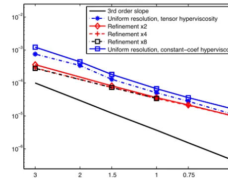
Figure 12. As in Fig. 11, except for TC5. In case of tensor-based
hyperviscosity, three error curves for grid refinement with×2,×4 or×8 local refinement are practically indistinguishable and obtain the same convergence rates as seen with uniform grids. For a given
1xlow, the presence of some local refinement (×2) does decrease
the global error, but×4 or×8 levels of local refinement produce no further benefit.
2 and 5, the scalar approach had noticeable noise and oscil-lations near regions of local mesh refinement, which was not present with the tensor formulation. Results for both formu-lations were sensitive to the grid quality, as shown by com-paring results on a highly distorted grid with sharp mesh transitions and a smooth grid with less acute angles due to its lower valence nodes. But, in TC2, the tensor formulation showed less grid sensitivity and obtained excellent results on both grids.
When running with tensor hyperviscosity in the SEM, the presence of local mesh refinement in TC2 had no impact on the global errors. The SEM obtained its formal order of ac-curacy for all grids tested (up to 8×regional refinement). In TC5, with refinement over the mountain, the presence of re-finement, again, did no harm to the global errors and actually resulted in a small improvement. Asymptotically, the global errors were controlled by the coarse resolution, and the lo-cally refined meshes obtained the same convergence rates as the global uniform meshes.
Appendix A: An element-local map for quadrilaterals on a sphere
Numerical methods for the sphere based on cubed-sphere grids need to define a mapr(x)from the reference element to the sphere (in the case of finite element methods) or from each cube face to the sphere for finite difference or finite element methods. Most approaches use the equidistant cen-tral projection (Sadourny, 1972), the equiangular cencen-tral pro-jection (Rancic et al., 1996), or their combination (Fournier et al., 2004). All three of these approaches were compared in Nair et al. (2005), where the equiangular mapping was found to be the most accurate. However, all three aforementioned projections are based on an inscribed cube and cannot cor-rectly treat elements lying across cube edges. In particular, for an edge of such an element, the reference element maps for the two elements that share this edge may not agree, re-sulting in a loss of the SEM’s mimetic properties. Here, we present a map that avoids this issue by using a map local to each element. The map uses a bilinear transformation based on elements’ physical coordinates and does not make use of an inscribed cube. It is similar to the map used for triangular elements in Lauter et al. (2008).
For each quadrilateral elementm on the surface of the
unit sphere, we denote the map and its inverse byr(x;m)
and x(r;m), where x=(x1, x2). To construct r(x;m), let c1,c2,c3, andc4be Cartesian coordinates of the vertices of mwithc1=(cx1, c1y, cz3)T, etc. and define
r=
er/kerk2
with
er=
1
4((1−x1)(1−x2)c1+(1+x1)(1−x2)c2+ (A1)
(1+x1)(1+x2)c3+(1−x1)(1+x2)c4) .
We now give an analytical expression for D=∂r/∂x, needed in Sect. 2. We use both Cartesian and longi-tude–latitude coordinates:
r=
cosλcosθ
sinλcosθ
sinθ !
whereλ∈ [0,2π], θ∈ [−π/2, π/2]. (A2)
Since dr=cosθdλeλ+dθeθ,, it follows that
D=
cosθ 0
0 1
∂(λ, θ )
∂x =
cosθ 0
0 1
∂(λ, θ )
∂r
∂r
∂x. (A3)
To avoid the singularity at the poles in the term
cosθ 0
0 1
∂(λ, θ )
∂r =
−
sinλ cosλ 0
0 0 cos1θ
,
we further decompose the term ∂∂xr =∂r ∂er
∂er
∂x, so that we can
extract a factor of cosθfrom ∂r∂ er
. Some algebra shows
∂r
∂er = 1
||
er||2
a11 a12 a13 a21 a22 a23 a31 a32 a33
,
where a11=sin2λcos2θ+sin2θ, a12= −12sin 2λcos2θ, a13= −12cosλsin 2θ, a21= −12sin 2λcos2θ, a22= cos2λcos2θ+sin2θ, a23= −12sinλsin 2θ, a31=
−1
2cosλsin 2θ,a32= − 1
2sinλsin 2θ, anda33=cos2θ. Also,
∂er
∂x = 1 4
cx1 cx2 cx3 cx4 cy1 cy2 cy3 cy4 c1z c2z c3z c4z
−1+x2 −1+x1 1−x2 −1−x1 1+x2 1+x1
−1−x2 1−x1
.
Altogether, we have
D= 1 ||er||2
1 4
−sinλ cosλ 0
0 0 1
·
a11 a12 a13
a21 a22 a23
a31/cosθ a32/cosθ a33/cosθ
·
c1x c2x c3x c4x c1y c2y c3y c4y cz1 cz2 cz3 cz4
−1+x2 −1+x1 1−x2 −1−x1 1+x2 1+x1
−1−x2 1−x1
, where
er=
1 4
cx1 cx2 cx3 cx4 cy1 cy2 cy3 cy4 c1z c2z c3z c4z
(1−x1)(1−x2) (1+x1)(1−x2) (1+x1)(1+x2) (1−x1)(1+x2)
Acknowledgements. This research was supported by the
Depart-ment of Energy Office of Biological and EnvironDepart-mental Research, work package no. 12-015334 – “Multiscale Methods for Accurate, Efficient, and Scale-Aware Models of the Earth System” – and work package no. 11-014996 – “Climate Science for a Sustainable En-ergy Future”. Sandia National Laboratories is a multi-program lab-oratory managed and operated by Sandia Corporation, a wholly owned subsidiary of Lockheed Martin Corporation, for the US De-partment of Energy’s National Nuclear Security Administration, un-der contract no. DE-AC04-94AL85000.
We would like to thank two anonymous reviewers for their suggestions, which significantly improved the manuscript. Edited by: H. Weller
References
Ainsworth, M. and Wajid, H.: Dispersive and dissipative behav-ior of the spectral element method, SIAM J. Numer. Anal., 47, 3910–3937, 2009.
Baer, F., Wang, H., Tribbia, J., and Fournier, A.: Climate model-ing with spectral elements, Mon. Weather Rev., 134, 3610–3624, 2006.
Blacker, T. D. and Stephenson, M. B.: Paving: a new approach to automated quadrilateral mesh generation, Int. J. Numer. Meth. Eng., 32, 811–847, 1991.
Boville, B.: Sensitivity of simulated climate to model resolution, J. Climate, 4, 469–485, 1991.
Dennis, J. M., Edwards, J., Evans, K. J., Guba, O., Lauritzen, P. H., Mirin, A. A., St.-Cyr, A., Taylor, M. A., and Worley, P. H.: CAM-SE: a scalable spectral element dynamical core for the Commu-nity Atmosphere Model, Int. J. High Perform. C., 26, 74–89, 2012.
Dobrev, V., Kolev, T., and Rieben, R.: High-order curvilinear finite element methods for Lagrangian hydrodynamics, SIAM J. Sci. Comput., 34, B606–B641, 2012.
Fournier, A., Taylor, M., and Tribbia, J.: The spectral element atmo-sphere model (SEAM): high-resolution parallel computation and localized resolution of regional dynamics, Mon. Weather Rev., 132, 726–748, 2004.
Lauter, M., Giraldo, F. X., Handorf, D., and Dethloff, K.: A discontinuous Galerkin method for the shallow water equa-tions in spherical triangular coordinates, J. Comput. Phys., 227, 10226–10242, 2008.
Marras, S., Kopera, M. A., and Giraldo, F. X.: Simulation of Shallow Water Jets with a Unified Element-based Continu-ous/Discontinuous Galerkin Model with Grid Flexibility on the Sphere, Q. J. Roy. Meteor. Soc., in press, 2014.
Nair, R. D., Thomas, S., and Loft, R.: A discontinuous Galerkin transport scheme on the cubed-sphere, Mon. Weather Rev., 133, 814–828, 2005.
Persson, P.-O. and Strang, G.: A simple mesh generator in MAT-LAB, SIAM Rev., 46, 329–345, 2004.
Rancic, M., Purser, R., and Mesinger, F.: A global shallow-water model using an expanded spherical cube: gnomonic versus con-formal coordinates, Q. J. Roy. Meteor. Soc., 122, 959–982, 1996. Ringler, T. D., Jacobsen, D., Gunzburger, M., Ju, L., Duda, M., and Skamarock, W.: Exploring a multi-resolution modeling ap-proach within the shallow-water equations, Mon. Weather Rev., 139, 3348–3368, 2011.
Sadourny, R.: Conservative finite-difference approximations of the primitive equations on quasi-uniform spherical grids, Mon. Weather Rev., 100, 136–144, 1972.
St.-Cyr, A., Jablonowski, C., Dennis, J. M., Tufo, H. M., and Thomas, S. J.: A comparison of two shallow water models with non-conforming adaptive grids, Mon. Weather Rev., 136, 1898–1922, 2008.
Takahashi, Y., Hamilton, K., and Ohfuchi, W.: Explicit global sim-ulation of the mesoscale spectrum of atmospheric motions, Geo-phys. Res. Lett., 33, L12812, doi:10.1029/2006GL026429, 2006. Taylor, M. A. and Fournier, A.: A compatible and conservative spec-tral element method on unstructured grids, J. Comput. Phys., 229, 5879–5895, 2010.
Weller, H., Weller, H. G., and Fournier, A.: Voronoi, Delau-nay, and block-structured mesh refinement for solution of the shallow-water equations on the sphere, Mon. Weather Rev., 137, 4208–4224, 2009.
Williamson, D. L., Drake, J. B., Hack, J. J., Jakob, R., and Swarz-trauber, P. N.: A standard test set for numerical approximations to the shallow water equations in spherical geometry, J. Comput. Phys., 102, 211–224, 1992.
Yu, M., Giraldo, F. X., Peng, M., and Wang, Z.: Localized arti-ficial viscosity stabilization of discontinuous Galerkin methods for nonhydrostatic mesoscale atmospheric modeling, J. Comput. Phys., in review, 2014.