www.geosci-model-dev.net/9/4155/2016/ doi:10.5194/gmd-9-4155-2016
© Author(s) 2016. CC Attribution 3.0 License.
A land surface model combined with a crop growth model for paddy
rice (MATCRO-Rice v. 1) – Part 2: Model validation
Yuji Masutomi1, Keisuke Ono2, Takahiro Takimoto3, Masayoshi Mano4, Atsushi Maruyama2, and Akira Miyata2
1College of Agriculture, Ibaraki University, 3-21-1, Chuo, Ami, Inashiki, Ibaraki 300-0393, Japan 2Institute for Agro-Environmental Sciences, NARO, 3-1-3, Kannondai, Tsukuba, Ibaraki 305-8604, Japan
3Institute for Global Change Adaptation Science, Ibaraki University, 3-21-1, Chuo, Ami, Inashiki, Ibaraki 300-0393, Japan 4Graduate School of Horticulture, Chiba University, 648 Matsudo, Matsudo-shi, Chiba 271-8510, Japan
Correspondence to:Yuji Masutomi ([email protected])
Received: 5 February 2016 – Published in Geosci. Model Dev. Discuss.: 19 February 2016 Revised: 16 October 2016 – Accepted: 7 November 2016 – Published: 21 November 2016
Abstract.We conducted two types of validation for the sim-ulations by MATCRO-Rice developed by Masutomi et al. (2016). In the first validation, we compared simulations with observations for latent heat flux (LHF), sensible heat flux (SHF), net carbon uptake by crop, and paddy rice yield from 2003 to 2006 at the site where model parameters are parame-terized. In the second validation, we compared the observed and simulated paddy rice yields over Japan from 1991 to 2010 between observations and simulations. The 4-year av-erage root mean square errors (RMSEs) of the first valida-tion for LHF and SHF were 18.20 and 15.47 W m−2, respec-tively. These values for errors are comparable to those re-ported in earlier studies. The comparison of biomass growth during growing periods from 2003 to 2006 at the parame-terization site shows that the simulations were in agreement with the observations, indicating that the model can repro-duce the net carbon uptake by crops well. The 4-year aver-age RMSE of the first validation for crop yield in the same period was 410.6 kg ha−1, which accounted for 8.1 % of the mean observed yields. The error of the second validation for crop yield was 16.7 % and the correlation of crop yields be-tween observations and simulations from 1991 to 2010 was significant at 0.663 (P <0.01). These results indicate that MATCRO-Rice has high ability to accurately and consis-tently simulate LHF, SHF, net carbon uptake by crop, and crop yield.
1 Introduction
It has been recognized that crop growth and management in agricultural land are important factors that affect climate at various spatial and temporal scales via exchange of heat, wa-ter, and gases (Tsvetsinskaya et al., 2001; Bondeau et al., 2007; Osborne et al., 2009; Levis et al., 2012). Betts (2005) pointed out that integration of crop growth models (CGMs) into climate models is needed for accurate climate simula-tions by climate models. To consider the influence of agricul-tural land on climate in climate simulations, several land sur-face models (LSMs) or dynamic vegetation models (DVMs) incorporated with a CGM have been developed (Tsvetsin-skaya et al., 2001; Kucharik, 2003; Gervois et al., 2004; Bon-deau et al., 2007; Osborne et al., 2007; Lokupitiya et al., 2009; Maruyama and Kuwagata, 2010; Levis et al., 2012; Osborne et al., 2015).
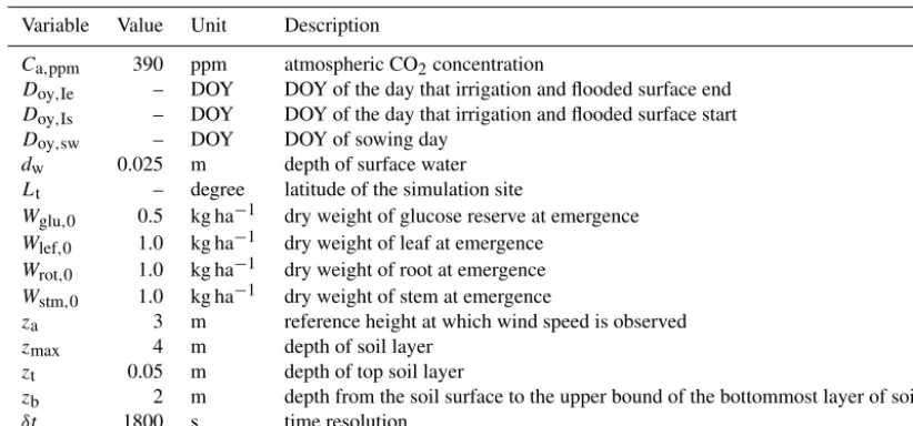
Table 1.Simulation setting parameters.
Variable Value Unit Description
Ca,ppm 390 ppm atmospheric CO2concentration
Doy,Ie – DOY DOY of the day that irrigation and flooded surface end Doy,Is – DOY DOY of the day that irrigation and flooded surface start
Doy,sw – DOY DOY of sowing day
dw 0.025 m depth of surface water
Lt – degree latitude of the simulation site
Wglu,0 0.5 kg ha−1 dry weight of glucose reserve at emergence Wlef,0 1.0 kg ha−1 dry weight of leaf at emergence
Wrot,0 1.0 kg ha−1 dry weight of root at emergence Wstm,0 1.0 kg ha−1 dry weight of stem at emergence
za 3 m reference height at which wind speed is observed
zmax 4 m depth of soil layer
zt 0.05 m depth of top soil layer
zb 2 m depth from the soil surface to the upper bound of the bottommost layer of soil
δt 1800 s time resolution
the understanding of the interaction is important for securing food security. However, little is known about the interaction. MATCRO-Rice can be a useful tool for studying the interac-tion between climate and paddy rice fields.
The objective of the present paper is to present the results of the comprehensive validation of MATCRO-Rice and to show the effects of modifications from the original LSM, MATSIRO. Before presenting the results of the validation and the effects of modification, we first show the numeri-cal method (Sect. 2) and the method and results of param-eterization for model parameters (Sect. 3). The results of model validation and the effects of modifications are shown in Sects. 4 and 5, respectively, followed by concluding re-marks in Sect. 6.
2 Numerical setting and method
All simulation setting parameters are shown in Table 1. We set the time resolution of the simulation to half an hour, i.e. δt=1800 s. For time discretization, the forward difference method was used.
To simulate soil water and heat transfer (Sect. 3.5 in Masu-tomi et al., 2016), we spatially discretized soil into five layers with thickness of 0.05, 0.2, 0.75, 1.0, and 2.0 m, resulting in zmax=4.0 m,zt=0.05 m, andzb=2.0 m. To simulate soil
water content for each soil layer (ws), we replaced the
gradi-ent of water flux by net water fluxes between layers. In the calculation for water fluxes between layers, we used the hy-draulic conductivity that is smaller among soil layers and the difference in water potentials between soil layers. After the calculation for soil water content for each layer, water con-tent beyond saturation was taken out to base flow.
To simulate soil temperature for each soil layer, we solved the system of equations for soil layers by using the Gauss–
Jordan method. In the calculation of soil temperatures, we replaced the gradient of heat flux by net heat fluxes between layers. In the calculation of heat fluxes between layers, we used thermal conductivity averaged between soil layers and soil temperatures for each layer.
The downhill simplex method (Nelder and Mead, 1965) was used to simulate temperatures of the canopy and surface (TcandTg; Sect. 3.1 in Masutomi et al., 2016), bulk transfer
coefficients (CEg,CEc,CHg,CHc,CM, andCMg; Sect. 3.3 in Masutomi et al., 2016), and variables related to carbon assimilation (An,x,ci,x, andgst,x; Sect. 4.1 in Masutomi et al., 2016).
We set za=3 m. CO2 concentration (Ca,ppm) and the
depth of surface water (dw) were set at 390 ppm and 0.025 m,
respectively. The initial dry weight of each organ was set at 1 kg ha−1for leaf (Wlef,0), stem (Wstm,0), and root (Wrot,0),
and at 0.5 kg ha−1for glucose reserve in the leaf (Wglu,0). Doy,Ie,Doy,Is,Doy,sw, andLt depend on the simulations.
Values for these parameters are shown in the sections of each simulation.
3 Parameterization
Table 2 shows model parameters parameterized in the present paper. All parameters are parameterized using observations, the literature, and assumptions. The method of the parame-terization is explained in this section.
3.1 Parameterization site and observation data
tempera-Table 2.Parameters parameterized.
Variable Value Unit Description
Dvs,rot1 0.1 – 1st point ofDvsat which the partition pattern to root changes
Dvs,rot2 Dvs,h – 2nd point ofDvsat which the partition pattern to root changes
Dvs,lef1 0.2 – 1st point ofDvsat which the partition pattern to leaf changes
Dvs,lef2 0.7 – 2nd point ofDvsat which the partition pattern to leaf changes
Dvs,pnc1 0.5 – 1st point ofDvsat which the partition pattern to panicle changes
Dvs,pnc2 0.7 – 2nd point ofDvsat which the partition pattern to panicle changes
Dvs,e 0.012 – Dvsat emergence
fstc 0.288 – fraction of glucose allocated to starch reserves
haa 0.439 – parameter for relationship between LAI and crop height before heading
hab 0.675 – parameter for relationship between LAI and crop height before heading
hba 0.366 – parameter for relationship between LAI and crop height after heading
hbb 0.318 – parameter for relationship between LAI and crop height after heading
Dvs,h 0.616 – Dvsat heading
kyld 0.675 – ratio of crop yield to dry weight of panicle at maturity
kSlw 3.5 – parameter that represents the relationship betweenSlwandDvs
Gds,m 167759940 K s growing degree second at maturity
Prot 0.25 – partition ratio of glucose to root
Plef 0.5 – partition ratio of glucose to leaf from glucose partitioned to the shoot
rd1,lef 5.0×10⁻⁷ s−1 ratio of leaf death at harvest
Slw,mx 600 kg m−2 maximum specific leaf area
Slw,mn 350 kg m−2 minimum specific leaf area
s1 0.045 K−1 temperature dependence ofVmax,xonVm,x
s2 328 K temperature dependence ofVmax,xonVm,x
Vmax(0) 0.001 mol m−2(l)s−1 reference value for maximum RuBisCO capacity at the canopy top
Dvs,tr 0.06 – Dvsat transplanting and at which transplanting shock starts
Dvs,te 0.08 – Dvsat which transplanting shock ends
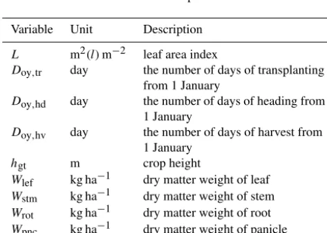
Table 3.Observational data used for parameterization.
Variable Unit Description
L m2(l)m−2 leaf area index
Doy,tr day the number of days of transplanting
from 1 January
Doy,hd day the number of days of heading from
1 January
Doy,hv day the number of days of harvest from 1 January
hgt m crop height
Wlef kg ha−1 dry matter weight of leaf Wstm kg ha−1 dry matter weight of stem Wrot kg ha−1 dry matter weight of root Wpnc kg ha−1 dry matter weight of panicle
Yld kg ha−1 yield
ture of 13.7◦C and precipitation of 1200 mm. The soil type is clay loam. The variety planted at the site isKoshihikari, which is the most planted variety in Japan.
Biomass for each organ (Wlef,Wpnc,Wrot, andWstm) and
leaf area index (L) were measured nearly every 2 weeks. At each measuring time, 10 stands were sampled from the fields. Yield (Yld) and phenological dates including
trans-planting (Doy,tr), heading (Doy,hd), and harvest (Doy,hv) were
observed every year. The values of observed yield are the husked rice yield with 15 % water content. The rice grains for measuring yield were sampled from the whole fields of the observational site. The crop height (hgt) was measured
on average every 5 days. 3.2 Phenology
Phenological parameters that represent development stages (Dvs,e,Dvs,h,Gds,m,Dvs,tr, andDvs,te) were parameterized.
First, we calculated Dvs values at heading and Gds,m
val-ues from 2003 to 2006 using the phenological model given by Masutomi et al. (2016). The mean values were set to Dvs,h and Gds,m, resulting in Dvs,h=0.616 and Gds,m=
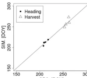
167759940 K s. Figure 1 compares the heading and harvest dates between observations and simulations from 2003 and those from 2006. The simulated heading and harvest dates were in good agreement with the observations. The average errors were 2.25 and 4.5 days for heading and harvest, re-spectively.
Dvs,e,Dvs,tr, andDvs,te were determined so that the
Figure 1.Comparison of heading and harvest dates. SIM: simula-tions; OBS: observasimula-tions; DOY indicates the number of days from 1 January.
3.3 Partitioning
MATCRO partitions carbohydrates in leaves, in the form of glucose, into each organ, according to MACROS (Penning de Vries et al., 1989). Parameters related to glucose partitioning (Dvs,rot1,Dvs,rot2,Dvs,lef1,Dvs,lef2,Dvs,pnc1,Dvs,pnc2,Prot,
and Plef) were parameterized as follows: (i) we calculated
the ratio of glucose partitioned to each organ (leaf, stem, root, panicle) during the growing period using the observed biomass for each organ; (ii) we conducted the curve fitting of the calculated ratios in (i). Figure 2 shows the calculated ra-tios of glucose partitioned to each organ and the fitting curves for the ratios.
To determine the ratio of dead leaves at harvest (rd1,lef),
we first calculated the observational ratios of dead leaves dur-ing growdur-ing periods by dividdur-ing the decrease in leaf biomass between observational dates by the duration among the ob-servational dates. Then, by graphically fitting a curve to the calculated ratios of dead leaves, we determined rd1,lef.
Fig-ure 3 shows the calculated ratios of dead leaves and the fitted curve.
The fraction of glucose allocated to starch reserve (fstc)
is determined as follows: (i) we first calculated the ratios of stem biomass at harvest to maximum stem biomass for each year from 2003 to 2006 (Bouman et al., 2001); (ii) then, a 4-year average was calculated forfstc.
3.4 LAI, crop height, and specific leaf weight
To obtain the parameters for the relationship between LAI and crop height (haa, hab, hba, andhbb), we conducted
lin-ear regressions of the data before and after heading using observations for LAI and crop height from 2003 to 2006. Thus, haa=0.439, hab=0.675, hba=0.366, and hbb=
0.318. Figure 4 compares the LAI–height relation between observations and simulations.
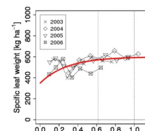
To obtain parameters for specific leaf weight (kSlw,Slw,mn, andSlw,mx), we plotted observations for specific leaf weights
during growing periods from 2003 to 2006 and conducted the
curve fitting of the plotted data. Thus,kSlw=3.5,Slw,mn= 350, and Slw,mx=600. Figure 5 shows the specific leaf
weights and the fitted curve.
3.5 Crop yield
To determine the ratio of crop yield to dry weight of pani-cle at harvest (kyld), we calculated the dry weight of panicle
at harvest, because the weight was not observed. By assum-ing linear increase of dry weight from the last date in which dry weight of the panicle was measured, we calculated the dry weight of the panicle at harvest from 2003 to 2006. The median value among the ratios of observed yields to the cal-culated dry weight of panicle producedkyld.
3.6 RuBisCO-limited photosynthesis rate
Parameters related to RuBisCO-limited photosynthesis rate (Vmax(0),s1, and s2) were parameterized using the values
obtained from the literature. In this parameterization, we ad-justed the parameters so that the RuBisCO-limited photo-synthesis rate (ωc,x) simulated by MATCRO agrees with the observational value reported by Borjigidai et al. (2006). In the simulations, CO2 concentration in the leaf was fixed to ci,x =30 Pa. Figure 6, showing the comparison of RuBisCO-limited photosynthesis rates among MATCRO, those re-ported by Borjigidai et al. (2006), and MATSIRO (Takata et al., 2003), on which MATCRO is based, indicates that there is a good agreement in the photosynthesis rate between the simulations of MATCRO and the observational value in Bor-jigidai et al. (2006); the simulations for the photosynthesis rate of MATCRO were significantly improved compared to those of MATSIRO.
4 Validation
We conducted two types of validation. The first validation was conducted at the parameterization site as explained in Sect. 3.1. In the validation, the simulated LHF, SHF, car-bon uptake by crop, and crop yields were compared with the observations from 2003 to 2006. The second validation was conducted for a territory across Japan. The simulated crop yields for Japan were compared with the national statistics from 1991 to 2010.
4.1 Validation at the parameterization site 4.1.1 Input and validation data
Figure 2.Partitioning ratio of glucose. Red lines are fitted.Dvsindicates the development stage.
Figure 3.Ratio of dead leaves. A red line is fitted.Dvsindicates the development stage.
Figure 4.Relationship between the leaf area index (LAI) and crop height (black curve:hgt=haaLhab; red curve:hgt=hbaLhbb).
above ground, because the reference height (za) is set to be
3 m (Sect. 3.1). It is noted that we used the observed values of photosynthetic active radiation (PAR) in addition to the standard meteorological inputs, because PAR, which is often not measured, was observed at the parameterization site. We setLt=36.05. Values for soil parameters for clay loam are
shown in Table 5. TheKoshihikari variety was planted us-ing a transplantus-ing technique. We setDoy,Is=114, 107, 114,
113, and Doy,Ie=231, 251, 243, 241 from 2003 to 2006,
respectively, using the observations for the depth of surface water (dwo).Doy,swwas calculated from the observed
trans-Figure 5.Relationship between specific leaf weight and develop-ment stage (Dvs). A red curve denotes the fitted curve used in the model.
Figure 6.RuBisCO-limited photosynthesis rate.
planting date (Doy,tr), assuming that transplanting was
con-ducted 20 days after sowing, i.e.Doy,sw=Doy,tr−20.
Table 4.Observational data used for validation at the parameterization site.
Variable Unit Description
Meteorological inputs
Pa Pa Air pressure
Pr kg m−2s−1 Precipitation
Q kg kg−1 Specific humidity
Rsd(0) W m−2 Downward shortwave radiant flux density at the canopy top Rld(0) W m−2 Downward longwave radiant flux density at the canopy top
Ta K Air temperature
U m s−1 Wind speed
D1d(0)+S1d(0) W m−2 Downward radiant flux density for photosynthetic active radiation at the canopy top
Management
dwo m Observed depth of surface water
Doy,tr DOY DOY of transplanting day
Outputs
λE W m−2 Latent heat flux
H W m−2 Sensible heat flux
L – LAI
Tg – Surface temperature
Wsh+Wrot kg ha−1 Total biomass
Yld kg ha−1 Yield
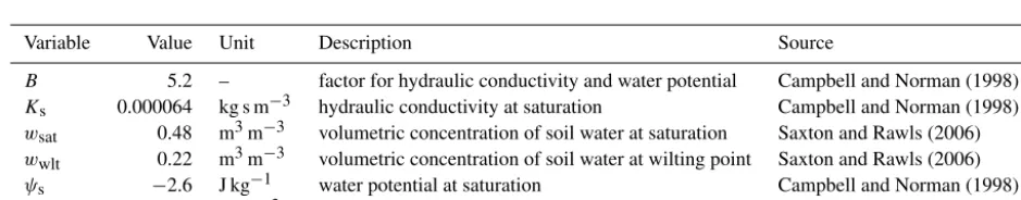
Table 5.Soil-type specific parameters.
Variable Value Unit Description Source
B 5.2 – factor for hydraulic conductivity and water potential Campbell and Norman (1998)
Ks 0.000064 kg s m−3 hydraulic conductivity at saturation Campbell and Norman (1998)
wsat 0.48 m3m−3 volumetric concentration of soil water at saturation Saxton and Rawls (2006) wwlt 0.22 m3m−3 volumetric concentration of soil water at wilting point Saxton and Rawls (2006)
ψs −2.6 J kg−1 water potential at saturation Campbell and Norman (1998)
ρs 1390 kg m−3 bulk density of soil Saxton and Rawls (2006)
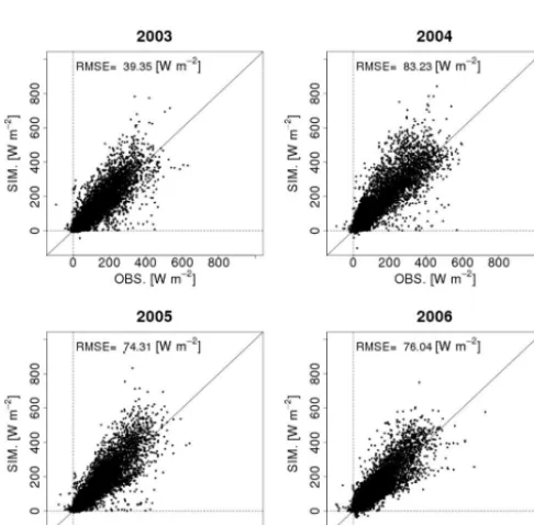
4.1.2 Comparison of LHF and SHF
Figures 7 to 10 show the comparison of the daily and half-hourly LHF and SHF from 2003 to 2006. We can observe that MATCRO can replicate the daily and half-hourly varia-tions in LHF and SHF accurately. Quantitatively, the RMSEs of daily LHF between simulations and observations for each year were 15.15, 21.84, 17.25, and 18.57 W m−2, with the 4-year average of 18.20 W m−2(Table 6). The RMSEs of daily SHF were 13.62, 14.72, 14.84, and 18.69 W m−2, with the
4-year average of 15.47 W m−2(Table 7). These RMSE values
are comparable to those reported in earlier studies (Kimura and Kondo, 1998; Maruyama and Kuwagata, 2010).
One of the major reasons for the errors of LHF and SHF between simulations and observations is thought to be a prob-lem in flux observations. Aubinet et al. (1999) reported that the energy balance in observations is not closed. In contrast, the energy balance simulated by MATCRO is completely
Table 6.RMSEs for daily LHF.
Model 2003 2004 2005 2006 Ave.
MATCRO 15.15 21.84 17.25 18.57 18.20
MATCRO 19.4 20.78 19.28 18.72 19.54
(fixed LAI)
MATCRO-RF 16.63 36.90 29.32 24.93 26.95
Table 7.RMSEs for daily SHF.
Model 2003 2004 2005 2006 Ave.
MATCRO 13.62 14.72 14.84 18.69 15.47
MATCRO 14.69 20.30 16.93 20.68 18.15
(fixed LAI)
Figure 7.Comparison of daily LHF between simulations and observations. DOY indicates the number of days from 1 January.
Figure 8.Comparison of half-hourly LHF between simulations and observations.
closed. Therefore, the energy imbalance in flux observations can cause errors between simulations and observations. El Maayar et al. (2008) suggested to test the degree of energy imbalance in observations before comparing the observations
with simulations. This degree is generally evaluated by
Im= X
d
H (d)+λE(d)
Rn(d)−G(d) !
/N, (1)
whereH,λE,Rn, and G are the daily averages for SHF,
LHF, net radiation, and heat flux into ground, respectively;d indicates a day; andN is the number of days. The observa-tion values forRnandGin this equation are expected to be
sufficiently accurate (Twine et al., 2000; Wilson et al., 2002). The values ofImin the observations from 2003 to 2006 were
Figure 9.Comparison of SHF between simulations and observations. DOY indicates the number of days from 1 January.
Figure 10. Comparison of half-hourly SHF between simulations and observations.
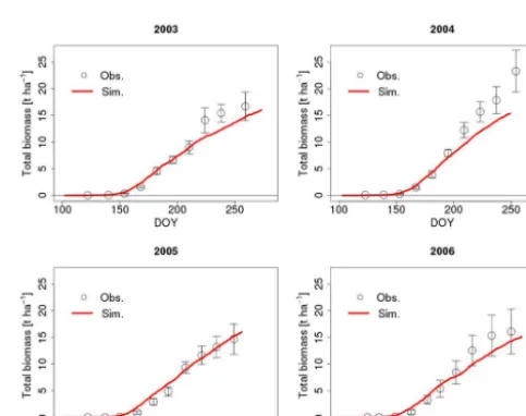
Hence, we conclude that the model has high accuracy for simulating net carbon uptake by crops during growing peri-ods.
Figure 11.Comparison of total biomass between simulations and observations during growing periods from 2003 to 2006. Circles in-dicate mean values of observations and the ranges inin-dicate standard deviation of observations. Red lines denote simulations. DOY indi-cates the number of days from 1 January.
4.1.4 Comparison of yield
Figure 12.Comparison of yields between simulations and observa-tions.
yields well. The mean RMSE from 2003 to 2006 was 410.6 kg ha−1, which was 8.1 % of the mean observed yields.
However, the model overestimated the crop yields in 2003. The primary cause of the large overestimation in 2003 can be attributed to the late harvest in the simulation for 2003; the model delayed the harvest by 11 days in 2003 (see Sect. 3.2). To confirm this, we recalculated the yield in 2003 by using the observed harvest date. The revised yield is shown in the figure as a red circle. The revised yield was in good agree-ment with the observations in 2003. These results suggest that the phenological model in MATCRO should be further improved for a more accurate estimation of crop yield. The current version of the phenological model in MATCRO im-plements only the temperature. The consideration of the pho-toperiod may further improve the accuracy of the phenologi-cal model in the simulation of harvest date as well as heading date (e.g. Penning de Vries et al., 1989; Connor et al., 2011).
4.2 Validation over Japan
4.2.1 Method, input, and validation data
Rice yields for all prefectures in Japan were simulated from 1991 to 2010, and then the average national rice yield was calculated for each year from the prefectural yields weighted by the prefectural planting areas. The simulated rice yields for Japan were compared with the national crop statistics (MAFF, 1991–2010).
The Global Meteorological Forcing Dataset (GMFD) for land surface modelling (Sheffield et al., 2006) was used for meteorological input data. Because the spatial resolution of the GMFD is 1◦, the average meteorological values for each prefecture were calculated from the gridded values weighted by the prefectural planting areas. The time resolution of the GMFD is 3 h. We used the same values every 3 h for half-hourly simulations. The comparison with the agrometeoro-logical dataset in Japan (Ohno et al., 2012) revealed that shortwave radiation of the GMFD has a large error; we cor-rected the error using the agrometeorological dataset, so that
Figure 13.Comparison of yields over Japan between simulations and observations.
the daily values for shortwave radiation of the GMFD could agree with those of the agrometeorological dataset. In addi-tion, we changed the ratio of photosynthetic active radiation to shortwave radiation from 0.5 (default) to 0.423, according to the value observed at the parameterization site (Sect. 3.1). The sowing and harvesting dates (Doy,swandDoy,hv) for
each prefecture were obtained from the national crop statis-tics (MAFF, 1991–2010). In this validation, simulated har-vesting dates were not used because the results in the pre-vious section (Sect. 4.1.4) showed that simulated harvesting dates may cause errors in yield simulations.
For simplicity, land surface was assumed to be annually flooded and irrigated. Hence, we setDoy,Is=1 andDoy,Ie=
365.Ltfor each prefecture was set to the latitude of the
cen-tre of each prefecture. The other simulation settings and pa-rameters for crops and soil were set using the values shown in Tables 1, 2, and 5.
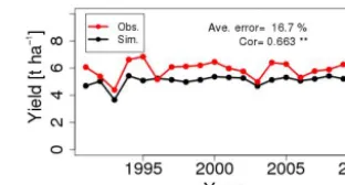
4.2.2 Comparison of yield
Figure 13 shows the comparison of the observed and sim-ulated yields from 1991 to 2010. The average error be-tween simulations and observations was 16.7 %. Although the simulated yields tended to overestimate the observa-tions, the correlation between simulations and observations was significant at 0.663 (P <0.01). Hence, we conclude that MATCRO can reproduce substantial parts of weather-induced variability in yields. One of the reasons for the sim-ulation errors is thought to be the method of parameteriza-tion. For the simulations over Japan, we used parameters parameterized for a varietyKoshihikarionly at one site in Japan (Sect. 3), although there is a large diversity in agricul-tural management and techniques, and rice varieties planted throughout Japan. Therefore, parameterization on a large scale is necessary for better large-scale simulations.
5 Effects of modifications
of LHF and SHF. Both simulations are conducted at the pa-rameterization site from 2003 to 2006 (Sect. 3.1).
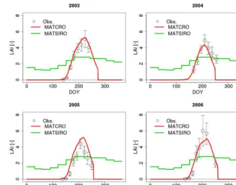
5.1 Effect of dynamic calculation of LAI
The original LSM (MATSIRO) uses the monthly constant LAI, which is given in gridded form. The default gridded LAI data of MATSIRO were obtained from the Global Soil Wetness Project 2 (Dirmeyer et al., 2006). Figure 14 shows the comparison of LAI between observations, simulations by MATCRO, and the default values of MATSIRO. We can see that MATCRO adequately reproduces seasonal changes in LAI, although the default LAI are not in agreement with the observed LAI. MATSIRO also uses constant crop height and root length, which are vegetation-specific parameters. The default values of crop height and root length for crops are 1 m. Using the default data for LAI and the default values for crop height and root length, we simulated LHF and SHF from 2003 to 2006. In the simulations, we also used the original equation of MATSIRO for calculating the maximum canopy water (wcap).
The RMSEs of daily LHF from 2003 to 2006 were 19.4, 20.78, 19.28, and 18.72 W m−2, respectively, with the 4-year average of 19.54 W m−2 (Table 6). The RMSEs of daily SHF from 2003 to 2006 were 14.69, 20.30, 16.93, and 20.68 W m−2, respectively, with the 4-year average of 18.15 W m−2(Table 7). These errors are comparable to those of MATCRO. Hence, we conclude that the effects of the dy-namic calculation of LAI, crop height, and root length on LHF and SHF are small.
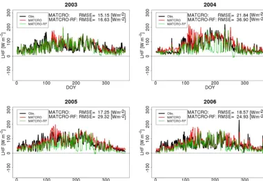
5.2 Effect of flooded and irrigated surface
We simulated LHF and SHF from 2003 to 2006 without flooded surface and irrigation. The simulations are called MATCRO-RF, which denotes simulations under rain-fed conditions. Figures 15 and 16 show the comparison of daily LHF and LHF between observations and simulations ob-tained by MATCRO and MATCRO-RF. The LHF and SHF simulated by MATCRO-RF were not in agreement with the observations. The RMSEs of daily LHF simulated by MATCRO-RF from 2003 to 2006 were 16.63, 36.90, 29.32, and 24.93 W m−2, respectively, with the 4-year average of 26.95 W m−2(Table 6). The RMSEs of daily SHF from 2003 to 2006 were 16.34, 42.02, 34.16, and 31.56 W m−2, respec-tively, with the 4-year average of 31.02 W m−2 (Table 7).
These errors in MATCRO-RF are considerably larger than those simulated by MATCRO. Figures 15 and 16 show that MATCRO-RF tends to underestimate daily LHF and to over-estimate daily SHF. The underestimation of daily LHF can be attributed to lower evaporation from the soil due to the ab-sence of irrigation and flooding. The overestimation of daily SHF can be caused by high surface temperature due to lower evaporation from the soil. Hence, we conclude that flooded
Figure 14.Comparison of LAI between observations, simulations by MATCRO, and the default value of MATSIRO.
surface and irrigation have large effects on simulations of LHF and SHF.
6 Concluding remarks
In this paper, we presented the results of the validation of MATCRO-Rice and the effects of the modification of the original LSM (MATSIRO), and the numeric and parameter-ization methods. First, the comparison of the LHF and SHF between simulations and observations at the paramerization site confirmed that the model can reproduce the observed LHF and SHF data well. The accuracy of the simulations for LHF and SHF was comparable to those obtained in earlier studies. Second, we showed that the simulated growth of the total biomass was in good agreement with the observations at the parameterization site. This indicates that the model can simulate the net carbon uptake by crops during a growing period at paddy rice fields. Last, we demonstrated that the model has high ability to simulate crop yield by comparing the simulated and observed yields at the parameterization site and over Japan.
Figure 15.Comparison of daily LHF between observations and simulations by MATCRO and MATCRO-RF. DOY indicates the number of days from 1 January.
We validated LHF, SHF, and carbon flux simulated by this model with observations from only one site. The model should be further validated at multiple sites in order to en-force the reliability and applicability of the model. However, since there are a few flux sites on agriculture land worldwide, it will be necessary to increase their number on agricultural land to promote climate–crop modelling studies.
We assessed the effects of the dynamic simulation of LAI, crop height, and root length on LHF and SHF and the effect of flooded surface and irrigation on LHF and SHF. The re-sults show that the effects of the dynamic simulation on LHF and SHF are small, whereas the flooded surface and irriga-tion have large effects on LHF and SHF. These results sug-gest that climate–crop modelling should incorporate flooded surface and irrigation.
7 Code and data availability
The source code of MATCRO will be distributed upon request to the corresponding author (Yuji Masutomi: [email protected]). The website for MATCRO-Rice will be developed in the near future.
Acknowledgements. We are grateful to E. Hatanaka for her help in the extensive literature survey. This research was supported by the Environment Research and Technology Development Fund (S-12) and the Program on Development of Regional Climate Change Adaptation Plans in Indonesia (PDRCAPI) of the Ministry of the Environment.
Edited by: T. Kato
Reviewed by: C. Müller and two anonymous referees
References
AsiaFlux: MSE: Mase paddy flux site, available at: http://asiaflux. net/index.php?page_id=83, last access: 5 February 2016. Aubinet, M., Grelle, A., Ibrom, A., Rannik, Ü., Moncrieff, J.,
Fo-ken, T., Kowalski, A. S., Martin, P. H., Berbigier, P., Bernhoffer, Ch., Clement, R., Elbers, J., Granier, A., Grünwald, T., Morgen-stern, K., Pilegaard, K., Rebmann, C., Snijders, W., Valentini, R., and Vesala, T.: Estimates of the annual net carbon and water exchange of forests: the EUROFLUX methodology, Adv. Ecol. Res., 30, 113–175, 1999.
Betts, R. A.: Integrated approaches to climate-crop modelling: needs and challenges, Philos. T. Roy. Soc. B, 360, 2049–2065, 2005.
Bondeau, A., Smith, P. C., Zaehle, S., Schaphoff, S., Lucht, W., Cramer, W., Gerten, D., Lotze-Campen, H., Müller, C., Reich-stein, M., and Smith, B.: Modelling the role of agriculture for the 20th century global terrestrial carbon balance, Glob. Change Biol., 13, 679–706, 2007.
Borjigidai, A., Hikosaka, K., Hirose, T., Hasegawa, T., Okada, M., and Kobayashi, K.: Seasonal changes in temperature dependence
of photosynthetic rate in rice under a free-air CO2enrichment, Ann. Bot., 97, 549–557, 2006.
Bouman, B. A. M., Kropff, M. J., Tuong, T. P., Wopereis, M. C. S., ten Berge, H. F. M., and van Laar, H. H.: ORYZA2000: modeling lowland rice, International Rice Research Institute and gen University and Research Centre, Phillippines and Wagenin- Wagenin-gen, the Netherlands, 2001.
Campbell, G. S. and Norman, J. M.: An introduction to environ-mental biophysics, Springer-Verlag, New York, USA, 1998. Connor, D. J., Loomis, R. S., and Cassman, K. G.: Crop
ecol-ogy: productivity and management in agricultural systems, Cam-bridge University Press, CamCam-bridge, UK, 2011.
Dirmeyer, P. A., Gao, X., Zhao, M., Guo, Z., Oki, G., and Hanasaki, N.: GSWP-2, Multimodel analysis and implications for out per-ception of the land surface, B. Am. Meteorol. Soc., 87, 1381– 1397, 2006.
El Maayar, M., Chen, J. M., and Price, D. T.: On the use of field measurements of energy fluxes to evaluate land surface models, Ecol. Model., 214, 293–304, 2008.
Gervois, S., de Noblet-Ducoudré, N., Viovy, N., Ciais, P., Brisson, N., Seguin, B., and Perrier, A.: Including croplands in a global biosphere model: methodology and evaluation at specific sites, Earth Interact., 8, 1–25, 2004.
Kimura, R. and Kondo, J.: Heat balance model over a vegetated area and its application to a paddy filed, J. Meteorol. Soc. Jpn., 76, 937–953, 1998.
Kucharik, C. J.: Evaluation of a process-based agro-ecosystem model (Agro-IBIS) across the U.S. corn belt: simulations of the interannual variability in maize yield, Earth Interact., 7, 1–33, 2003.
Levis, S., Bonan, G. B., Kluzek, E., Thornton, P. E., Jones, A., Sacks, W. J., and Kucharik, C. J.: Interactive crop management in the Community Earth System Model (CESM1): Seasonal in-fluences on land-atmosphere fluxes, J. Climate, 25, 4839–4859, 2012.
Lokupitiya, E., Denning, S., Paustian, K., Baker, I., Schaefer, K., Verma, S., Meyers, T., Bernacchi, C. J., Suyker, A., and Fischer, M.: Incorporation of crop phenology in Simple Biosphere Model (SiBcrop) to improve land-atmosphere carbon exchanges from croplands, Biogeosciences, 6, 969–986, doi:10.5194/bg-6-969-2009, 2009.
Maruyama, A. and Kuwagata, T.: Coupling land surface and crop growth models to estimate the effects of changes in the growing season on energy balance and water use of rice paddies, Agr. Forest Meteorol., 150, 919–930, 2010.
Masutomi, Y., Takahashi, K., Harasawa, H., and Matsuoka, Y.: Im-pact assessment of climate change on rice production in Asia in comprehensive consideration of process/parameter uncertainty in general circulation models, Agr. Ecosyst. Environ., 131, 281– 291, 2009.
Masutomi, Y., Ono, K., Mano, M., Maruyama, A., and Miyata, A.: A land surface model combined with a crop growth model for paddy rice (MATCRO-Rice v. 1) – Part 1: Model description, Geosci. Model Dev., 9, 4133–4154, doi:10.5194/gmd-9-4133-2016, 2016.
Nelder, J. A. and Mead, R.: A simplex method for function mini-mization, Comput. J., 7, 308–313, 1965.
Ohno, H., Sasaki, K., Yoshida, H., Nakazono, K., and Nak-agawa, H.: 1 km Mesh Agrometeorological Data and the Environment for High-levelUsage, NARO, Tsukuba, avail-able at: http://www.naro.affrc.go.jp/project/results/laboratory/ narc/2012/210a10143.html, 2012 (in Japanese).
Osborne, T., Gornall, J., Hooker, J., Williams, K., Wiltshire, A., Betts, R., and Wheeler, T.: JULES-crop: a parametrisa-tion of crops in the Joint UK Land Environment Simulator, Geosci. Model Dev., 8, 1139–1155, doi:10.5194/gmd-8-1139-2015, 2015.
Osborne, T. M., Lawrence, D. M., Challinor, A. J., Slingo, J. M., and Wheeler, T. R.: Development and assessment of a coupled crop-climate model, Glob. Change Biol., 13, 169–183, 2007. Osborne, T. M., Slingo, J., Lawrence, D., and Wheeler, T.:
Exam-ining the interaction of growing crops with local climate using a coupled crop-climate model, J. Climate, 22, 1393–1411, 2009. Penning de Vries, F. W. T., Jansen, D. M., ten Berge, H. F. M., and
Bakema, A.: Simulation of ecophysiological processes of growth in several annual crops, Centre for Agricultural Publishing and Documentation (Poduc), Wageningen, the Netherlands, 1989. Saxton, K. E. and Rawls, W. J.: Soil water characteristic estimates
by texture and organic matter for hydrologic solutions, Soil Sci. Soc. Am. J., 70, 1569–1578, 2006.
Sheffield, J., Goteti, G., and Wood, E. F.: Development of a 50-yr high-resolution global dataset of meteorological forcings for land surface modelling, J. Climate, 19, 3088–3111, 2006.
Takata, K., Emori, S., and Watanabe, T.: Development of the minimal advanced treatments of surface interaction and runoff, Global Planet. Change, 38, 209–222, 2003.
Tsvetsinskaya, E. A., Mearns, L. O., and Easterling, W. E.: Inves-tigating the effects of seasonal plant growth and development in three-dimensional atmospheric simulations. Part II: Atmospheric response to crop growth and development, J. Climate, 14, 711– 729, 2001.
Twine, T. E., Kustas, W. P., Norman, J. M., Cook, D. R., Houser, P. R., Meyers, T. P., Prueger, J. H., Starks, P. J., and Wesely, M. L.: Correcting eddy-covariance flux underestimates over a grassland, Agr. Forest Meteorol., 103, 279–300, 2000.