The Subgrid Importance Latin Hypercube Sampler (SILHS): a multivariate subcolumn generator

(1)

Geosci. Model Dev., 6, 1813–1829, 2013 www.geosci-model-dev.net/6/1813/2013/ doi:10.5194/gmd-6-1813-2013

Geoscientific

Model Development

Open Access

The Subgrid Importance Latin Hypercube Sampler (SILHS):

a multivariate subcolumn generator

V. E. Larson and D. P. Schanen

Department of Mathematical Sciences, University of Wisconsin – Milwaukee, Milwaukee, WI, USA

Correspondence to: V. E. Larson ([email protected])

Received: 18 January 2013 – Published in Geosci. Model Dev. Discuss.: 19 March 2013 Revised: 30 August 2013 – Accepted: 12 September 2013 – Published: 29 October 2013

Abstract. Coarse-resolution climate and weather forecast models cannot accurately parameterize small-scale, nonlin-ear processes without accounting for subgrid-scale ity. To do so, some models integrate over the subgrid variabil-ity analytically. Although analytic integration methods are attractive, they can be used only with physical parameteriza-tions that have a sufficiently simple functional form. Instead, this paper introduces a method to integrate subgrid variability using a type of Monte Carlo integration. The method gener-ates subcolumns with suitable vertical correlations and feeds them into a microphysics parameterization. The subcolumn methodology requires little change to the parameterization source code and can be used with a wide variety of physical parameterizations.

Our subcolumn generator is multivariate, which is impor-tant for physical processes that involve two or more hydrom-eteor species, such as accretion of cloud droplets by rain drops. In order to reduce sampling noise in the integrations, our subcolumn generator employs two variance-reduction methods, namely importance and stratified (Latin hypercube) sampling. For this reason, we name the subcolumn generator the Subgrid Importance Latin Hypercube Sampler (SILHS).

This paper tests SILHS in interactive, single-column sim-ulations of a marine stratocumulus case and a shallow cu-mulus case. The paper then compares simulations that use SILHS with those that use analytic integration. Although the SILHS solutions exhibit considerable noise from time step to time step, the noise is greatly damped in most of the time-averaged profiles.

1 Introduction

Large-scale models of the atmosphere typically parameter-ize subgrid-scale physical processes, such as microphysics or radiative transfer. A typical physical parameterization es-timates the rate of a process at a point in space, whereas a coarse-resolution model instead needs the process rate av-eraged over a grid-box scale. Therefore, there is a benefit to upscaling point process rates to grid-box averages by ac-counting for subgrid-scale variability. Accurate upscaling is of potential importance for any process that involves signif-icant small-scale spatial variability and is highly nonlinear. For instance, upscaling is expected to benefit nonlinear mi-crophysical processes such as the autoconversion of cloud droplets to raindrops and the accretion of liquid cloud water by falling raindrops.

In many cases, the problem of upscaling reduces to the problem of performing integrals such as the following:

hf (x, y)i =

Z

P (x, y)f (x, y)dxdy. (1)

Here,x andy are fields that vary over a grid box, such as liquid cloud water and rain mixing ratios;P (x, y)is the subgrid probability density function (PDF) that provides the probability density that particular values of x andy occur within a particular grid box and time step; andf (x, y)is a function representing the process to be integrated, such as autoconversion or accretion. For illustration, we have written Eq. (1) as a bivariate function ofx andy, but in principle, any number of variates could be used.

(2)

1814 V. E. Larson and D. P. Schanen: The Subgrid Importance Latin Hypercube Sampler

cite two methods, namely analytic integration and Monte Carlo integration:

1. Analytic integration. If both the PDF, P (x, y), and the process rate function,f (x, y), are sufficiently sim-ple analytic functions, then the integralhf (x, y)imay be performed analytically. Numerous papers have per-formed such integrals in order to compute the liquid cloud fraction using an assumption of instantaneous saturation adjustment (e.g., Sommeria and Deardorff, 1977; Mellor, 1977; Smith, 1990; Lewellen and Yoh, 1993; Bony and Emanuel, 2001; Tompkins, 2002). Other papers have used analytic integration in order to upscale microphysical process rates (e.g., Zhang et al., 2002; Morrison and Gettelman, 2008; Cheng and Xu, 2009; Larson and Griffin, 2013; Griffin and Larson, 2013; Weber and Quaas, 2012).

Advantages of analytic integration include the facts that the integrals so obtained are exact and entail rela-tively little computational expense. Disadvantages in-clude the facts that deriving such integrals is time-consuming and the facts that complicated process rate functions, including numerical algorithms, cannot be integrated analytically.

2. Monte Carlo integration. A second way to perform the integral in Eq. (1) is to use Monte Carlo integra-tion. That is, one may draw a sample ofx andy that is distributed according to the PDF P (x, y), evalu-ate the process revalu-atef (x, y)at those points, and aver-age the resulting sample of process rates. Monte Carlo integration has been applied to radiative transfer pa-rameterizations by the Monte Carlo independent col-umn approximation (McICA) (e.g., Barker et al., 2002; Pincus et al., 2003; Räisänen et al., 2004; Räisänen and Barker, 2004; Räisänen et al., 2005; Pincus et al., 2006). A type of Monte Carlo integration has also been recommended for use with microphysics (Larson et al., 2005; Larson, 2007). A similar but deterministic sam-pling strategy is used in the Tripleclouds parameteri-zation (Shonk and Hogan, 2008; Shonk et al., 2012). A disadvantage of Monte Carlo integration is the sam-pling noise that is inherent in the use of a necessar-ily limited number of sample points. However, these sampling errors have been found to be of relatively little consequence in tests of McICA (Pincus et al., 2003; Räisänen et al., 2005; Pincus et al., 2006; Räisä-nen et al., 2007; Barker et al., 2008; RäisäRäisä-nen et al., 2008). Nevertheless, in order to reduce the sampling errors, variance-reduction techniques have been intro-duced for the McICA (Räisänen and Barker, 2004; Hill et al., 2011). Another method to reduce noise is the use of stratified sampling, in which sample points are cho-sen such that they are spread out and do not clump (Larson et al., 2005).

An advantage of Monte Carlo integration is that it can be applied quite generally to complicated process rates f (x, y), including those that are numerical algorithms. Furthermore, Monte Carlo integration is non-intrusive; in other words, it allows the integral to be performed without requiring modification to the computer code that implements the point process rate f (x, y). This is possible because Monte Carlo integration separates and distinguishes the representation of subgrid vari-ability from the calculation of local physical processes. Therefore, Monte Carlo integration might be particu-larly useful for models like the Weather Research and Forecasting (WRF) model (Skamarock et al., 2005) that contain many options for physics parameteriza-tions, and also useful for models whose physics pack-ages are updated frequently.

Another advantage of some Monte Carlo integrators is that they allow a variety of assumptions about the cor-relation of sample points in the vertical, including both random and maximal overlap of vertical points. Flex-ibility of the vertical correlations is useful for driving radiative transfer parameterizations and diagnostic pa-rameterizations of precipitation.

This paper describes and presents tests of a new Monte Carlo integration method called the Subgrid Importance Latin Hypercube Sampler (SILHS). SILHS generates a dis-tribution of sample points that permits efficient Monte Carlo integration of integrals such as Eq. (1). The process rate func-tion f (x, y) must be supplied separately by, for instance, a microphysics scheme. In addition, the PDF P (x, y) in Eq. (1) must be provided separately by, for instance, a cloud and turbulence parameterization such as the Cloud Layers Unified By Binormals (CLUBB) parameterization (Golaz et al., 2002; Larson and Golaz, 2005). Unlike previous Monte Carlo generators, which focused mostly on calculating cloud overlap and generating profiles of liquid cloud water, SILHS is used here to generate profiles of rain water and vertical velocity, along with profiles of liquid cloud water.

(3)

V. E. Larson and D. P. Schanen: The Subgrid Importance Latin Hypercube Sampler 1815

SILHS generates vertical profiles of sample points, al-lowing the integral in Eq. (1) to be computed at each grid level. SILHS therefore may be called a subcolumn gener-ator. SILHS uses both importance and stratified sampling in order to perform variance reduction, that is, to reduce sampling noise. SILHS provides an option to choose sam-ple points preferentially within an important region, namely clouds containing liquid. SILHS also spreads out (i.e., strat-ifies) the sample points within the cloudy and clear regions separately using Latin hypercube sampling (McKay et al., 1979; Press et al., 1992; Owen, 2003; Gentle, 2003; Larson et al., 2005).

The remainder of this paper is organized as follows. In Sect. 2, we discuss the methodology behind SILHS, includ-ing the treatment of vertical overlap of clouds, reduction of noise, and multivariate correlations. In Sect. 2 we also briefly outline two other numerical models we use in conjunction with SILHS, namely CLUBB and a microphysics scheme (Khairoutdinov and Kogan, 2000). In Sect. 3, we compare the results of simulations that use Monte Carlo integration of the microphysics with those that use analytic integration for both a cumulus and a stratocumulus case. In Sect. 4, we present conclusions and provide a future outlook.

2 Methodology

This section describes the algorithm behind SILHS, first pro-viding an overview of the role that SILHS plays within a single-column model, and then providing more detail on how subcolumns are generated.

The following overview describes the four major steps that our single-column model undertakes in a single time step:

1. Construct the multivariate PDF of subgrid-scale

vari-ability (performed by CLUBB). In our approach,

sam-ple points are drawn from an underlying PDF. This PDF is computed separately from SILHS and provided as input to SILHS. In this paper, the PDF is calculated by CLUBB, which is described in Golaz et al. (2002) and Larson and Golaz (2005). In this paper, CLUBB’s PDF contains the following variates: vertical velocity w; total water mixing ratio (vapor + liquid)rt; liquid

water potential temperatureθl; rain mixing ratiorr; and

rain drop number mixing ratioNr. The two rain

vari-ates are distributed according to a single lognormal, whereas the other variates are distributed according to a two-component normal mixture. (A two-component normal mixture is the sum of two normal distributions, i.e., a double Gaussian PDF. The normal-mixture ter-minology is widely used in statistics.)

2. Draw a sample of subcolumns from the subgrid PDF

(performed by SILHS). Once the PDF has been

cal-culated by CLUBB, a sample of subcolumns for each

grid column is drawn from it. The generation of sub-columns is done by SILHS. SILHS is designed so that in the limit of an infinite number of sample columns per grid column and time step, the sample statistics converge to the desired vertical correlations, to the desired marginal PDF at each grid level, and to the desired horizontal (i.e., within grid box) correlations between variates. (The marginal PDF of, for exam-ple, variate x is the PDF that remains when the full multivariate PDF is integrated over all variates other thanx.) Because CLUBB computes a separate multi-variate PDF at each vertical grid level (rather than a single grid-column PDF, as in Larson, 2007), CLUBB does not provide any information about vertical corre-lations. Instead, the vertical overlap of the variates is handled by SILHS.

3. Feed subcolumns into microphysics and compute

mi-crophysical tendencies (performed by a microphysics parameterization). Each subcolumn is fed, one by one,

into a microphysics parameterization, which again is separate from CLUBB and SILHS. The micro-physics parameterization remains unaltered and does not “know” that the profiles being fed to it are from subcolumns rather than grid-box means. The micro-physics simply computes local quantities (such as au-toconversion, accretion, and evaporation) on the as-sumption that there is no heterogeneity within the sub-column (i.e., that at each grid level in a subsub-column, all fields are horizontally uniform). The microphysics cal-culates a separate set of microphysical tendencies for each subcolumn.

4. Average microphysical tendencies from each

subcol-umn in order to form a grid-box average. Finally,

the microphysical tendencies from all the subcolumns within a grid column are averaged together, using a weighted mean if necessary (described further below). The resulting grid-box-averaged profile of microphys-ical tendencies is fed back into the host model (in this case CLUBB) and used to update the grid-box means. In this way, the subcolumns provide a means for the microphysics to interact with the subgrid variability provided by CLUBB.

Background to the present paper can be found in Larson et al. (2005), which describes a predecessor to SILHS. In that paper, Latin hypercube samples were drawn from CLUBB and fed into a simple autoconversion formula, but the simu-lations described there did not use a complete microphysics parameterization and had no feedback from the autoconver-sion back to CLUBB.

(4)

2.1 Constructing the multivariate PDF of subgrid-scale variability

In order to compute the subgrid PDF from which SILHS draws sample points (step 1 in Sect. 2 above), this paper uses CLUBB (Golaz et al., 2002; Larson and Golaz, 2005; Larson et al., 2012). CLUBB computes the subgrid PDF by prog-nosing various higher-order central moments and making an assumption about the shape of the PDF. The prognostic equa-tions contain much of the physics of the combined CLUBB– SILHS model. The prognosed higher-order moments include variances of turbulent and thermodynamic quantities (w,rt,

andθl), covariances of those same quantities, and the

third-order moment of vertical velocity. The framework of the prognostic equations is derived directly from the governing equations of fluid flow by forming higher-moment equations and Reynolds-averaging them. However, many of the indi-vidual terms within those equations are parameterized. Be-cause these equations are prognostic, they contain some de-gree of memory of the state of the flow at a prior time step. The variances determine the width of the PDF; the covari-ances are related to the correlations between variates, and the third-order moment determines whether the PDF is skewed to low or high values. The moments, along with the assump-tion that the PDF has a normal-mixture/lognormal funcassump-tional form, determine the PDF for each grid box and time step. We omit further details about CLUBB’s formulation because it has been described in previous papers (Golaz et al., 2002; Larson and Golaz, 2005; Larson et al., 2012).

The CLUBB (and SILHS) source code, along with separate documentation, is freely downloadable for non-commercial use at http://clubb.larson-group.com/. CLUBB and SILHS are written entirely in Fortran 95 and can be compiled using a number of Fortran compilers on the Linux operating system. Both CLUBB and SILHS are contained within a single subversion (svn) code repository. The simu-lations described and shown in this paper were created with revision 4895 of the source code. Further documentation and instructions for running CLUBB and SILHS are contained in several README files that are included along with the source code. These files serve collectively as a user manual. Readers who are interested in details of the algorithm are en-couraged to peruse the source code. We have strived to write well-structured code that is annotated generously with code comments.

2.2 Drawing a sample of subcolumns from the subgrid PDF

In this subsection, we detail step two in Sect. 2, namely, the method by which sample points are drawn from the PDF of subgrid variability. In overview, the sampling strategy is to generate a uniformly distributed sample at a particular altitude of interest within the domain; then, starting from that altitude of interest, choose a vertically correlated profile

of sample points; and finally, transform the uniformly dis-tributed sample points to the PDF at each level calculated by CLUBB.

In our case, the PDF of interest is a single multivariate PDF with normal-mixture marginals forw,rt, and θl, and

single lognormal marginals forrrandNr(Larson and Griffin,

2013). A normal-mixture marginalP (x)of a generic variate xhas the following functional form:

P (x)=aP1(x)+(1−a)P2(x), (2)

wherea is the mixture fraction and a normal component is given by

Pi(x)=

1 (2π )1/2σexp

"

−(x−µ)2

2σ2

#

. (3)

Hereµandσ2are the mean and the variance, respectively, of x. The mean and variance may differ between components.

A lognormal marginalP (x)ofxhas the form

P (x)= 1

(2π )1/2σ xexp "

−(lnx−µ)2 2σ2

#

. (4)

Hereµandσ2are the mean and the variance, respectively, of lnx, and lnx is normally distributed. A lognormal shape was chosen because it contains only positive values, which is appropriate for hydrometeors. It has plausible tails, and the mathematics to handle an arbitrary number of correlated lognormal variates is tractable. A multivariate lognormal is tractable because a multivariate normal is straightforward mathematically, and the normal and lognormal distributions are related by simple exponentiation (Garvey, 2000).

As seen in Eq. (4), a 1-D lognormal functional form is specified by two parameters, which can be related by a sim-ple transformation to the lognormal’s mean and variance (Garvey, 2000, Appendix B). The means ofrrandNrare

cal-culated by the microphysics parameterization in use. SILHS diagnoses the variances ofrr andNr as being proportional

to the mean squared. For example, we set r02

r /rr2 equal to

a constant everywhere throughout the simulation. The values of the constants of proportionality that we choose, for the ma-rine stratocumulus case discussed below, are listed in Table 1 of Larson and Griffin (2013). These values are based on a large-eddy simulation. In order to improve the results for the shallow cumulus case discussed below, we increaseN02

r /Nr

2

within cloud to 2.2; below cloud, we decreaseN02

r /Nr

2

and r02

r /rr2to 1. A simple proportionality seems unlikely to be

accurate in all cases, particularly when the mean is large, but using a proportionality is computationally inexpensive and has some support from satellite observations (M. Lebsock, personal communication, 2012).

(5)

variates. In nature, these correlations vary with time and space. However, in order to maintain simplicity and reduce computational cost, we have prescribed the horizontal corre-lations in the present paper (see further details below). The values of the horizontal correlations that this paper uses are based loosely on large-eddy simulations. For the marine stra-tocumulus case discussed below, we use the values of corre-lations listed in Table 1 of Larson and Griffin (2013). We use the same correlation values for the shallow cumulus case dis-cussed below, except that, to improve the results for cumulus, the correlation between the extended liquid water,s(Larson et al., 2005), and the droplet number is set to zero. Prescrib-ing constant horizontal correlations in the simulations is not ideal because correlations are not constant in nature (Larson et al., 2011). In future work, one could attempt to diagnose the correlations at each time step, using a methodology such as that described in Larson et al. (2011).

The procedure by which SILHS generates subcolumns can be divided into the following five tasks:

1. Choose a starting grid level for sampling

As discussed below, we impose vertical correlations by choosing a sample value at one grid level, mov-ing to an adjacent vertical level, choosmov-ing a new but similar sample value, and so forth. The starting grid level can be any grid level (e.g., the lowermost level). However, if the starting grid level is far from a liq-uid cloud layer, then, because sample points gradually de-correlate with vertical distance, we cannot expect to choose sample points preferentially within liquid cloud, as we desire.

In order to mitigate this problem partly, we choose the starting grid level to be the level with the greatest liq-uid water mixing ratio. This does not help when a grid column contains, for instance, a large-liquid, stratocu-mulus layer and a small-liquid custratocu-mulus layer. How-ever, it does help for grid columns that contain, for in-stance, a single cumulus layer. If no liquid is present at any level, then we choose the grid level that is half the maximum grid level. Although our tests seem to in-dicate that our criterion for choosing the starting grid level is acceptable, this is an area that is in need of further experimentation, particularly for grid columns with multiple, distinct cloud layers. In such cases, one could choose different starting grid levels for different subcolumns, thereby sampling preferentially to some degree within multiple layers.

2. Generate an uncorrelated multivariate sample at the

starting grid level

Once the starting grid level is chosen, SILHS gener-ates for that level an uncorrelated, multivariate sample. The distribution lies between (0,1) and is uniform ex-cept for weightings discussed below. Stated differently,

SILHS generates a vector of independent, uniformly distributed sample points, each element of which cor-responds to a separate variate, such as w. Once the starting grid level is chosen, SILHS generates for that level an uncorrelated, multivariate sample. (The uncor-related, uniformly distributed samples are transformed to correlated, normally distributed ones in task 4 be-low.)

Care must be taken in sampling the variates that have two mixture components, namelyw,rt, andθl. In order

to ensure that the two mixture components are sam-pled in an unbiased way, SILHS assigns each sample point to one mixture component or the other accord-ing to the relative weights of the two mixture com-ponents. For concreteness, suppose that the weight of the first component is mixt_frac and the weight of the second is 1-mixt_frac. To assign the sample point to a component, SILHS generates an extra random vari-ate,X_u_dp1, that is uniformly distributed between 0 and 1 (see p. 56 of Johnson, 1987, and Larson et al., 2005). Then SILHS chooses the first component if X_u_dp1<mixt_frac and chooses the second com-ponent otherwise. All further discussion in this sub-section pertains to a single mixture component. Although the points are drawn from a uniform distri-bution, the sampling procedure of SILHS is compli-cated slightly by the fact that SILHS uses both impor-tance sampling and stratified sampling in order to re-duce noise.

First, if liquid cloud fraction is small at the starting grid level, then SILHS contains the option to sam-ple preferentially within an important region, namely cloud containing some liquid (Räisänen and Barker, 2004); therefore SILHS does importance sampling (Gentle, 2003). SILHS concentrates sample points within liquid/mixed-phase cloud because regions with liquid often contain considerable variability, and much interesting microphysics occurs there. In particular, if liquid cloud fraction exceeds 0.5, then SILHS does not sample preferentially within cloud, but if liquid cloud fraction lies between 0.001 and 0.5, then SILHS chooses an equal number of sample points within liq-uid cloud (i.e., where s >0) and outside of liquid cloud (i.e., wheres <0) for each mixture component. Because the samples are drawn preferentially from liq-uid cloud in grid boxes with low cloud fraction, SILHS must weight the sample points appropriately by liquid cloud fraction in order to ensure that grid-box aver-ages are unbiased. Namely, the weights outside of liq-uid cloud are given by

1−(cloud fraction at starting grid level)

(6)

and the weights within liquid cloud are given by

cloud fraction at starting grid level

(number of samples)/2 . (6) At this initial step in the algorithm, the sample points are generated according to a uniform distribution within liquid cloud and a uniform distribution out-side of cloud. To generate uniformly distributed points, SILHS uses the Mersenne twister algorithm (Mat-sumoto and Nishimura, 1998).

When liquid cloud fraction at the starting grid level lies between 0.001 and 0.5, SILHS chooses half the sample points within liquid cloud. If one were inter-ested only in within-cloud processes, such as auto-conversion and accretion, one could choose all points within cloud. However, some interesting processes do occur outside of cloud, such as evaporation of rain-drops falling alongside sheared cumulus clouds and clear-sky radiative transfer. Therefore, SILHS chooses some sample points outside of cloud.

In a second measure to reduce noise, SILHS employs stratified sampling. Stratified sampling spreads sam-ple points in order to avoid the clumping of points that naturally arises due to statistical chance. In particular, SILHS uses Latin hypercube sampling separately in both the cloudy and cloud-free regions. The method-ology behind Latin hypercube sampling is thoroughly described in many sources (e.g., McKay et al., 1979; Press et al., 1992; Owen, 2003; Gentle, 2003; Larson et al., 2005). In most applications, Latin hypercube sampling guarantees that sample points are spread out (i.e., stratified), but CLUBB–SILHS does not neces-sarily prohibit clumping of sample points. The reason is the following. CLUBB uses a two-component mix-ture for some variates. For those variates, SILHS guar-antees that the points assigned to particular component are stratified, but SILHS does not guarantee that the collection of points from both components, taken to-gether, are stratified. In other words, SILHS does not attempt to ensure that, say, a high-percentile sample value chosen from one component with a low mean ex-ceeds a low-percentile sample value chosen from the high-mean component. Nevertheless, SILHS’s Latin hypercube sampling does usually increase stratifica-tion of sample points.

3. Generate vertically correlated profiles of sample

points

Cloud parcels at different altitudes within a grid-column-sized volume are said to be “vertically over-lapped” if one cloud parcel resides vertically above the other. The vertical overlap of clouds strongly in-fluences cloud albedo (e.g., Morcrette and Fouquart,

1986). Two possible overlap assumptions are maxi-mum overlap, in which cloud fields are stacked verti-cally to the greatest extent possible, and random over-lap. These assumptions have the drawback of intro-ducing spurious dependence on the vertical grid spac-ing. In recent years, several authors have assumed that clouds are overlapped according to a weighted average of maximum and random overlap (Hogan and Illingworth, 2000; Bergman and Rasch, 2002; Räisänen et al., 2004; Pincus et al., 2005; Barker, 2008; Shonk et al., 2010; Oreopoulos et al., 2012). The weight of the maximum overlap component is assumed to decrease exponentially with distance be-tween the layers, with an e-folding length that needs to be determined. The e-folding length may vary with hydrometeor type (Pincus et al., 2005), meteorologi-cal regime (Pincus et al., 2005), and/or latitude (Shonk et al., 2010; Oreopoulos et al., 2012).

SILHS adopts a related but different approach. SILHS does not assume that the points are a weighted aver-age of maximum and random overlap but does choose sample points that decorrelate exponentially with in-creasing vertical distance between sample points: vert_corr=exp(−vert_decorr_coef1z /Lscale) . (7) Here vert_corr is not the correlation itself between points in the vertical, but vert_corr does increase with increasing correlation, as will become clear momen-tarily. The quantity 1zis the distance between grid levels, Lscale is CLUBB’s turbulent mixing length, and vert_decorr_coef is a constant number that allows SILHS to adjust the degree of vertical overlap and is provisionally set to 0.03 in this paper. Given a uni-formly distributed random number,X_u(k), between 0 and 1 at grid levelk, SILHS chooses the value at an ad-jacent grid level (e.g.,X_u(k+1)) according to a uni-form distribution that is centered on the valueX_u(k) and has a half-width of 1−vert_corr. IfX_u(k+1)lies outside(0,1), then the value is folded back so that it does lie within(0,1). That is, ifX_u(k+1) >1, then we setX_u(k+1)=2−X_u(k+1); ifX_u(k+1) <0, then we setX_u(k+1)= −X_u(k+1). Such corre-lated vertical profiles are built for each variate, includ-ing the extraX_u_dp1 variate that determines the mix-ture component. For simplicity, each variate uses the same value of vert_corr, even though in nature the ver-tical correlations of all quantities may not necessarily be equal.

(7)

Lscale (see Eq. 7). When Lscale is large, then parcels are allowed to travel further in the vertical direction (Golaz et al., 2002), which we assume is indicative of higher vertical coherence. This link between CLUBB’s mixing length and the decorrelation length introduces an approximate but interactive, dynamical aspect into the diagnosis of vertical overlap.

Ensuring that the samples are drawn from the desired means, variances, and covariances at each grid level is accomplished later by the transformation from a uni-form distribution to a normal-mixture/lognormal dis-tribution described below. Note that SILHS directly in-fluences only the vertical correlation of uniformly dis-tributed points and not the normal-mixture/lognormal points. Although the vertical correlations of the normal-mixture/lognormal points are related to those of uniformly distributed points, they are usually not equal.

4. Transform uncorrelated, uniformly distributed points

to correlated, normally distributed points

At this point in the algorithm, SILHS has generated multiple subcolumns of uncorrelated, uniformly dis-tributed (but weighted) sample points. Furthermore, SILHS has assigned each sample point to a mixture component by the aforementionedX_u_dp1 variate. SILHS now transforms these samples to a normal-mixture distribution with the desired horizontal corre-lations. Even the hydrometeor variates, which are ulti-mately transformed to single lognormal distributions, are transformed here to a normal-mixture distribution (with identical means and variances in each mixture component so that the distribution collapses to a single normal).

First, SILHS transforms the sample points for each mixture component from an uncorrelated uniform dis-tribution to an uncorrelated standard normal distribu-tion xstnd (i.e., a normal distribution with zero mean

and unit variance). This transformation is accom-plished by use of the inverse cumulative distribution function (Johnson, 1987; Larson et al., 2005). Second, we transformxstnd to a normally distributed sample,

xnonstnd, with the desired subgrid covariance matrix.

The purpose is to take into account the (horizontal) correlations among variates. The covariance matrix de-pends on the mixture component to which the sample point is assigned, but this mixture component is iden-tified by theX_u_dp1 variate. To transform the sam-ple points from standard normal to non-standard nor-mal, we use the commonly adopted formula (Johnson, 1987, pp. 52–54)

xnonstnd=Lcovxstnd+µ, (8)

whereµis the vector of means of the normal-mixture component and the matrix Lcov is the Cholesky

de-composition of the matrix of subgrid (horizontal) co-variances among all variates, includingw,rt,θl, and

all hydrometeors. For the lognormal variates (i.e., the hydrometeors),µis not the vector of means of the log-normal variates but rather the means of lnxnonstnd, such

that whenxnonstndis exponentiated, the desired means

of the lognormal variates are recovered (see Eq. 4). To do so, we use formulas from Garvey (2000) and Lar-son and Griffin (2013). In a similar fashion, for lognor-mal variates, the covariances associated with Lcovhave

been transformed from the lognormal space to a nor-mal space (Garvey, 2000; Larson and Griffin, 2013). Computing the Cholesky decomposition of the covari-ance matrix, Lcov, at each time step and for each grid

box would be excessively expensive. To avoid this cost and simplify the formulation, we prescribe the horizontal correlations between hydrometeors as fixed constants for all grid boxes and time steps. To do so, given the correlations, we compute the Cholesky de-composition of the correlation matrix, Lcorr. Because

the correlations are constant, Lcorr needs to be

com-puted only once at the beginning of a simulation. We transform Lcorr to the Cholesky decomposition of the

covariance matrix, Lcov, by row multiplication of Lcorr

by the standard deviation,σ (i)of each variatei: Lcov(i, j )=σ (i)Lcorr(i, j ). (9)

This multiplication does need to occur at each time step, but the multiplication is much cheaper than per-forming a Cholesky decomposition.

5. Exponentiate certain hydrometeor variates in order to

transform them to lognormal distributions

CLUBB and SILHS assume that hydrometeor variates such asrrandNrobey single lognormal distributions.

These variates are transformed from normal to log-normal distributions by exponentiation of the sample points. A single, rather than double, lognormal results because previously we assumed the same mean for each of the two components of a given hydrometeor species, and also the same variance.

2.3 Feeding subcolumns into microphysics and computing microphysical tendencies

The subcolumns can, in principle, be fed into a variety of physics parameterizations if so desired, thereby driving the parameterized physical processes with subgrid variability. However, in this paper, we feed the subcolumns only into a microphysics parameterization.

(8)

Disussion

P

ap

er

|

Disussion

P

ap

er

|

Disussion

P

ap

er

|

Disussion

P

ap

er

|

200 400 600 800 1000 1200 1400 0

0.01 0.02 0.03 0.04 0.05 0.06 0.07

Rain Water Path

Time [min]

rwp [kg/m

2]

analytic silhs_2 silhs_4 silhs_8 silhs_64

200 400 600 800 1000 1200 1400 0

5 10 15

x 10−3 Liquid Water Path

Time [min]

lwp [kg/m

2 ]

Fig. 1. Time series of rain water path (upper) and liquid water path (lower) from the RICO shallow cumulus case. Five different integrations of the microphysics are overplotted: analytic (orange dashed), and SILHS-based sampling with 2 points (light blue solid), 4 points (purple dot dashed), 8 points (dark blue solid), and 64 points (red dashed) per grid box and time step.32

Fig. 1. Time series of rain water path (upper) and liquid water

path (lower) from the RICO shallow cumulus case. Five different integrations of the microphysics are overplotted: analytic (orange dashed line), and SILHS-based sampling with 2 points (light blue solid line), 4 points (purple dot-dashed line), 8 points (dark blue solid line), and 64 points (red dashed line) per grid box and time step.

of Khairoutdinov and Kogan (2000). The Khairoutdinov– Kogan (KK) parameterization was formulated based on a de-tailed simulation of a shallow marine stratocumulus cloud and does not contain ice. In our simulations, we prescribe cloud droplet number mixing ratio. The KK parameteriza-tion prognoses both rain mixing ratio and rain number mix-ing ratio. One could compute the sedimentation term in the rain budget equation separately for each subcolumn, but for simplicity, this paper computes the sedimentation term only once using grid-box mean profiles. However, the grid-mean sedimentation velocity, which is used in sedimentation term, is obtained by averaging sedimentation velocities computed separately for each subcolumn.

The advantage for this paper of using the KK microphysics parameterization is that the KK process rates are formulated in terms of power laws, which can be integrated analyti-cally over CLUBB’s PDF (Larson and Griffin, 2013; Grif-fin and Larson, 2013). Simulations that use analytic integra-tion will provide a reference against which we will compare

Disussion

P

ap

er

|

Disussion

P

ap

er

|

Disussion

P

ap

er

|

Disussion

P

ap

er

|

100 200 300

0 0.005 0.01 0.015 0.02 0.025

Rain Water Path

Time [min]

rwp [kg/m

2]

100 200 300 0.04

0.06 0.08 0.1 0.12 0.14 0.16

Liquid Water Path

Time [min]

lwp [kg/m

2]

Fig. 2. As in Fig. 1, but for the DYCOMS-II RF02 marine stratocumulus case. Using more sample points reduces the noise.

33

Fig. 2. As in Fig. 1, but for the DYCOMS-II RF02 marine

stratocu-mulus case. Using more sample points reduces the noise.

simulations that use the SILHS Monte Carlo integrations. In the limit of an infinite number of sample points, the SILHS integration should converge to the analytic integration. 2.4 Averaging microphysical tendencies from each

subcolumn in order to form a grid-box average

To allow SILHS to be interactive, the subcolumn microphysi-cal tendencies must be fed back into the grid-box mean equa-tions of the host model, which, in this case, is CLUBB (see step 4 in Sect. 2). The averaging of the microphysical tenden-cies from each sample point is a straightforward calculation that needs to be inserted into the host model. Because sub-columns are chosen preferentially within cloud, the averages must be appropriately weighted according to cloud fraction.

3 Results

(9)

Disussion

P

ap

er

|

Disussion

P

ap

er

|

Disussion

P

ap

er

|

Disussion

P

ap

er

|

0 1 2 3 4

0 500 1000 1500 2000 2500 3000 3500 4000 4500

Cloud Fraction

cloud_frac [%]

Height [m]

0 2 4 6 8 10

x 10−6

0 500 1000 1500 2000 2500 3000 3500 4000 4500

Cloud Water Mixing Ratio, r c

rcm [kg/kg]

Height [m]

0 0.05 0.1 0.15

0 500 1000 1500 2000 2500 3000 3500 4000 4500

Variance of w

wp2 [m2/s2]

Height [m]

0 1 2 3

x 10−6

0 500 1000 1500 2000 2500 3000 3500 4000 4500

Rain Water Mixing Ratio, r r

rrainm [kg/kg]

Height [m]

Fig. 3. Profiles of cloud fraction (upper left), cloud liquid mixing ratio (upper right), variance of vertical

velocity (lower left), and rain mixing ratio (lower right) from the RICO shallow cumulus simulation.

Five different integrations of the microphysics are overplotted: analytic (orange dashed), and

SILHS-based sampling with 2 points (light blue solid), 4 points (purple dot dashed), 8 points (dark blue solid),

and 64 points (red dashed) per grid box and time step. Profiles are averaged over the last 12 hours of

the simulation. Averaged over 12 hours, the noise manifested in the time series (Fig. 1) is significantly

smoothed, except in rain mixing ratio itself.

34

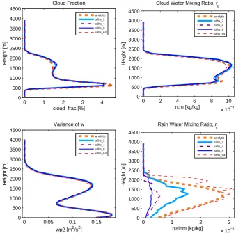
Fig. 3. Profiles of cloud fraction (upper left), cloud liquid mixing ratio (upper right), variance of vertical velocity (lower left), and rain

mixing ratio (lower right) from the RICO shallow cumulus simulation. Five different integrations of the microphysics are overplotted: analytic (orange dashed line), and SILHS-based sampling with 2 points (light blue solid line), 4 points (purple dot-dashed line), 8 points (dark blue solid line), and 64 points (red dashed line) per grid box and time step. Profiles are averaged over the last 12 h of the simulation. Averaged over 12 h, the noise manifested in the time series (Fig. 1) is significantly smoothed, except in rain mixing ratio itself.

the Ocean (RICO) field experiment (Rauber et al., 2007). The initial profiles, forcings, and surface fluxes of our configura-tion follow the GEWEX Cloud System Study (GCSS) spec-ifications for the RICO case (vanZanten et al., 2011). The other case involves a drizzling marine stratocumulus cloud observed during Research Flight 2 (RF02) of the Second Dy-namics and Chemistry of Marine Stratocumulus (DYCOMS-II) field experiment (Stevens et al., 2003). Our configuration again follows GCSS specifications (Wyant et al., 2007). As per GCSS specifications, for the RICO simulation, surface latent and sensible heat fluxes are computed interactively in terms of surface wind speed, temperature, and water vapor mixing ratio, whereas for the DYCOMS-II RF02 simula-tion, the surface fluxes are prescribed. Both the RICO and DYCOMS-II RF02 cases were simulated using a 5 min time step, and both used a stretched vertical grid with 128 levels and a vertical grid spacing of about 100 m at 1000 m altitude.

Figures 1 to 4 display results from 5 single-column simu-lations that are configured identically, except that one uses 2 sample points per grid box and time step (light blue solid line), another 4 points (purple dot-dashed line), another 8 points (dark blue solid line), another 64 points (red dashed line), and the final forgoes SILHS and instead integrates the microphysics analytically over the PDF (orange dashed line). The CLUBB simulations with analytic integrations serve as reference simulations to which the corresponding CLUBB– SILHS solutions should converge. Comparing the CLUBB– SILHS simulations to the CLUBB simulations with analytic integration allows us to isolate the effect of noise in the simu-lations from unrelated model errors in CLUBB. The analytic integration methodology is described in Larson and Griffin (2013) and Griffin and Larson (2013).

(10)

1822 V. E. Larson and D. P. Schanen: The Subgrid Importance Latin Hypercube SamplerDisussion

P

ap

er

|

Disussion

P

ap

er

|

Disussion

P

ap

er

|

Disussion

P

ap

er

|

0 20 40 60 80 100

0 200 400 600 800 1000 1200

Cloud Fraction

cloud_frac [%]

Height [m]

0 1 2 3

x 10−4

0 200 400 600 800 1000 1200

Cloud Water Mixing Ratio, r c

rcm [kg/kg]

Height [m]

0.05 0.1 0.15 0.2 0.25

0 200 400 600 800 1000 1200

Variance of w

wp2 [m2/s2]

Height [m]

0 0.5 1 1.5 2

x 10−5

0 200 400 600 800 1000 1200

Rain Water Mixing Ratio, r r

rrainm [kg/kg]

Height [m]

Fig. 4. As in Fig. 3, except for the DYCOMS-II RF02 marine stratocumulus simulation. Profiles are averaged over the full duration of the simulation (6 hours). Averaged over 6 hours, the noise manifested in the time series (Fig. 2) is considerably smoothed in all fields.

35

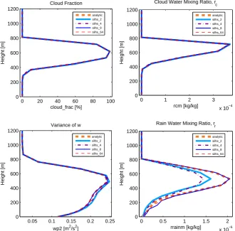
Fig. 4. As in Fig. 3, except for the DYCOMS-II RF02 marine stratocumulus simulation. Profiles are averaged over the full duration of the

simulation (6 h). Averaged over 6 h, the noise manifested in the time series (Fig. 2) is considerably smoothed in all fields.

substantial noise in part because it is updated directly by SILHS’s microphysical tendencies, and this injection of noise at each time step is not overcome by negative feed-backs and diffusion of rain. Liquid water, on the other hand, is influenced only indirectly by noise from subcolumns. As a result, subcolumn noise is felt more strongly by rain than liquid water. Rain exhibits diminished but still considerable noise even when 64 sample points per grid box and time step are used (red dashed line). However, large-eddy simulations of shallow cumulus clouds with∼5 km×5 km domains also exhibit noise in horizontally averaged liquid water path and rain water path.

Although the time series exhibit considerable noise from time step to time step, this noise is not evident in most pro-files when they are averaged over long time periods. Fig-ure 3 shows profiles from RICO averaged over 12 h, and Fig. 4 shows profiles from DYCOMS-II RF02 averaged over 6 h. We did not use longer averaging periods because longer periods would span too much of the diurnal cycle. In both cases, the noise is greatly reduced in cloud fraction, liq-uid cloud water mixing ratio (rc), and variance of vertical

velocity (w02_{). One exception is profiles of rain water}

mix-ing ratio for RICO, which do not match the analytic solution even when 64 points are used. RICO fields are noisier than those in DYCOMS-II RF02 because RICO, being a cumu-lus case, has greater horizontal variability. Nevertheless, the noise in rain, which is directly updated by the subcolumn mi-crophysics tendencies, does not infect the long time averages of cloud and turbulence fields, which are not directly updated by the subcolumns. Moreover, the plots (and other unshown tests) show that the SILHS solution gradually approaches the analytic solution as more sample points are used, which is an important property. We note that if a simulation uses a time step longer than 5 min we used, then a longer averaging time will be necessary to reduce sampling noise.

(11)

Disussion

P

ap

er

|

Disussion

P

ap

er

|

Disussion

P

ap

er

|

Disussion

P

ap

er

|

200 400 600 800 1000 1200 1400 0

0.005 0.01 0.015 0.02 0.025

Rain Water Path

Time [min]

rwp [kg/m

2]

analytic silhs_2 det_cloud det_cloud_rain

100 200 300

0 0.005 0.01 0.015 0.02 0.025

Rain Water Path

Time [min]

rwp [kg/m

2 ]

analytic silhs_2 det_cloud det_cloud_rain

Fig. 5. Time series of rain water path from the RICO shallow cumulus simulation (upper panel) and from the DYCOMS-II RF02 marine stratocumulus simulation (lower panel). Shown are an analytic in-tegration of the microphysics (orange dashed), SILHS-based sampling with 2 points (light blue solid), deterministic use of the within-cloud liquid cloud water mixing ratio (green dashed), and deterministic use of within-cloud liquid and rain mixing ratio (black solid). In the RICO case, treating liquid determin-istically but not rain still permits sampling noise in the rain; treating both liquid and rain determindetermin-istically leads to an underprediction of rain.

₃₆

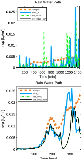
Fig. 5. Time series of rain water path from the RICO shallow

cu-mulus simulation (upper panel) and from the DYCOMS-II RF02 marine stratocumulus simulation (lower panel). Shown are an ana-lytic integration of the microphysics (orange dashed line), SILHS-based sampling with 2 points (light blue solid line), determinis-tic use of the within-cloud liquid cloud water mixing ratio (green dashed line), and deterministic use of within-cloud liquid and rain mixing ratio (black solid line). In the RICO case, treating liquid de-terministically but not rain still permits sampling noise in the rain; treating both liquid and rain deterministically leads to an underpre-diction of rain.

for RICO and II RF02 in Fig. 5. For DYCOMS-II RF02, all results are similar, because this cloud is fairly homogeneous. For RICO, however, calculating liquid deter-ministically but sampling rain leads to as much noise as sam-pling both liquid and rain. However, calculating both liquid and rain deterministically leads to an underprediction of rain. This indicates that accounting for the non-zero variance of rain is important in the RICO case because of nonlinearity in the rain processes.

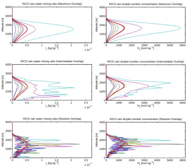
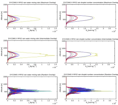
Examples of the vertical overlapping of profiles produced by SILHS are shown in Fig. 6. This figure shows pro-files of rain mixing ratio, rr, and rain number mixing

ra-tio,Nr, for RICO. The maximally overlapped profiles (upper

panel), which use vert_corr=1 in Eq. (7), are smooth be-cause SILHS attempts to maximize the vertical correlations

while preserving the grid-box means and variances at each grid level. The randomly overlapped profiles (lower panel) show no correlation between adjacent vertical grid levels, ex-cept the correlation that is inherent in following the vertical trend of the mean profiles. The intermediately overlapped profiles (middle panel), which use vert_decorr_coef=0.03 in Eq. (7), show an intermediate degree of vertical correla-tion. A separate, desirable feature of these profiles is that, collectively, they preserve the strong positive correlation be-tweenrr (left figure column) and Nr (right figure column)

that has been imposed by Eq. (8). The correlation betweenrr

andNris depicted by the color coding of the subcolumns, so

that, for instance, the blue lines correspond to therrandNr

variates of the same (multivariate) subcolumn. We see that for each subcolumn, when rris large,Nrtends to be large

as well, as desired for positively correlated variates. Simi-lar vertical overlap properties are exhibited for DYCOMS-II RF02 (see Fig. 7). For ease of interpretation, in these plots, SILHS does not preferentially sample within cloud but in-stead chooses each subcolumn with equal probability, so that each thin line on the plot has equal weight.

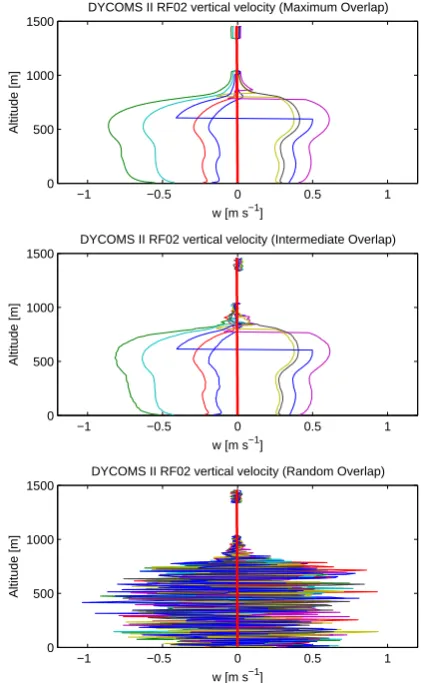
In comparison to the profiles of rr andNr, the vertical

overlapping of profiles of vertical velocity, w, has differ-ent properties owing to the fact that w is distributed ac-cording to a two-component normal mixture (see Fig. 8 for RICO and Fig. 9 for DYCOMS-II RF02). Namely, the pro-files with maximal overlap are smooth except for a small number of discrete jumps. These jumps in the profiles occur when the mixture component from which the sample point is drawn switches from one component to the other. The switch in components occurs because, in a maximally over-lapped profile, the extra variate that determines the choice of mixture component,X_u_dp1, is constant with altitude, but the weight of the first normal component, mixt_frac, varies with altitude. If the profile of mixt_frac crosses the value of X_u_dp1, then a jump in the profile will occur. The jumps are unrealistic but are difficult to avoid if an unbiased distri-bution and a two-component mixture are to be preserved.

(12)

Disussion

P

ap

er

|

Disussion

P

ap

er

|

Disussion

P

ap

er

|

Disussion

P

ap

er

|

0 0.5 1 1.5 2 2.5

x 10−5 0

1000 2000 3000 4000

RICO rain water mixing ratio (Maximum Overlap)

r

r [kg kg −1

]

Altitude [m]

0 1000 2000 3000 4000 5000 6000

0 1000 2000 3000 4000

RICO rain droplet number concentration (Maximum Overlap)

N

r [num kg −1

]

Altitude [m]

0 0.5 1 1.5 2 2.5

x 10−5 0

1000 2000 3000 4000

RICO rain water mixing ratio (Intermediate Overlap)

r

r [kg kg −1

]

Altitude [m]

0 1000 2000 3000 4000 5000 6000

0 1000 2000 3000 4000

RICO rain droplet number concentration (Intermediate Overlap)

N

r [num kg −1

]

Altitude [m]

0 0.5 1 1.5 2 2.5

x 10−5 0

1000 2000 3000 4000

RICO rain water mixing ratio (Random Overlap)

r

r [kg kg −1

]

Altitude [m]

0 1000 2000 3000 4000 5000 6000

0 1000 2000 3000 4000

RICO rain droplet number concentration (Random Overlap)

N

r [num kg −1

]

Altitude [m]

Fig. 6. A sample of eight equally weighted SILHS-generated profiles (thin lines) and the analytic

grid-box mean profile (thick red line) drawn from a single time step during the RICO shallow cumulus

simu-lation. (Importance sampling is foregone for the purpose of illustration in Figs. 6 through 9.) The vertical

correlation within each profile is specified to be maximal (upper panels), intermediate (middle panels),

or random (lower panels). Plotted are the rain mixing ratio (left figure column) and rain number mixing

ratio (right figure column) fields from the same eight profiles. The color coding of the sample profiles

is the same in both figure columns. By comparing lines of the same color in both the right-hand and

left-hand halves of the figure, one may see that the profiles of rain mixing ratio and number mixing ratio

are highly correlated to each other. This result is expected because high correlation is specified in these

simulations. The degree of vertical overlap in SILHS can be adjusted as desired between maximal and

random.

37

Fig. 6. A sample of eight equally weighted SILHS-generated profiles (thin lines) and the analytic grid-box mean profile (thick red line)

drawn from a single time step during the RICO shallow cumulus simulation. (Importance sampling is foregone for the purpose of illustration in Figs. 6 through 9.) The vertical correlation within each profile is specified to be maximal (upper panels), intermediate (middle panels), or random (lower panels). Plotted are the rain mixing ratio (left figure column) and rain number mixing ratio (right figure column) fields from the same eight profiles. The color coding of the sample profiles is the same in both figure columns. By comparing lines of the same color in both the right-hand and left-hand halves of the figure, one may see that the profiles of rain mixing ratio and number mixing ratio are highly correlated to each other. This result is expected because high correlation is specified in these simulations. The degree of vertical overlap in SILHS can be adjusted as desired between maximal and random.

relative costs of SILHS, CLUBB, and the microphysics are presented in Table 1.

4 Discussion and conclusions

In this paper, we have presented a new method, implemented in a software package called “SILHS”, that generates sub-columns for atmospheric models. The subsub-columns, once gen-erated, are fed into a microphysics parameterization, and the microphysical tendencies so produced are averaged and used to update the grid-box mean fields. We have tested SILHS in 1-D simulations of a shallow cumulus layer and a stratocu-mulus layer. In these two simulations, although SILHS does introduce noise into rain water mixing ratio, this noise does

not significantly degrade the time averages of liquid cloud water, cloud fraction, or other fields.

SILHS allows users to choose the number of sample points per grid box and time step. Increasing the number of sam-ple points reduces statistical noise but increases the compu-tational cost. We suspect that most users of SILHS with com-putational constraints will choose to use two sample points per grid box and time step. Even with only two sample points, SILHS allows the microphysics to sample both the clear-sky and within-cloud variability, thereby avoiding errors such as the systematic biases that result when convex or concave functions are fed grid-box means (e.g., Cahalan et al., 1994; Larson et al., 2001).

(13)

P

ap

er

|

Disussion

P

ap

er

|

Disussion

P

ap

er

|

Disussion

P

ap

er

|

0 0.2 0.4 0.6 0.8 1 1.2 1.4

x 10−4 0

500 1000 1500

DYCOMS II RF02 rain water mixing ratio (Maximum Overlap)

r_r [kg kg−1]

Altitude [m]

0 0.5 1 1.5 2 2.5 3 3.5 4

x 105 0

500 1000 1500

DYCOMS II RF02 rain droplet number concentration (Maximum Overlap)

N_r [num kg−1]

Altitude [m]

0 0.2 0.4 0.6 0.8 1 1.2 1.4

x 10−4 0

500 1000 1500

DYCOMS II RF02 rain water mixing ratio (Intermediate Overlap)

r_r [kg kg−1]

Altitude [m]

0 0.5 1 1.5 2 2.5 3 3.5 4

x 105 0

500 1000 1500

DYCOMS II RF02 rain droplet number concentration (Intermediate Overlap)

N_r [num kg−1]

Altitude [m]

0 0.2 0.4 0.6 0.8 1 1.2 1.4

x 10−4 0

500 1000 1500

DYCOMS II RF02 rain water mixing ratio (Random Overlap)

r

r [kg kg −1

]

Altitude [m]

0 0.5 1 1.5 2 2.5 3 3.5 4

x 105 0

500 1000 1500

DYCOMS II RF02 rain droplet number concentration (Random Overlap)

N

r [num kg −1

]

Altitude [m]

Fig. 7. As in Fig. 6, but for the DYCOMS-II RF02 marine stratocumulus simulation. The profiles of rain

mixing ratio and number mixing ratio have only moderate correlation, as specified by the user.

38

Fig. 7. As in Fig. 6, but for the DYCOMS-II RF02 marine stratocumulus simulation. The profiles of rain mixing ratio and number mixing

ratio have only moderate correlation, as specified by the user.

Table 1. Relative computational expense of SILHS, CLUBB, and

the KK microphysics. Two sample points per grid box and time step are drawn. The cost of SILHS is broken into various sub-costs. This simulation was run on a single processor. The code was compiled using the SunStudio Fortran compiler under the Linux operating system, and the timing was performed by Sun Analyzer 7.9.

Code portion % computational expense

CLUBB 50 %

Microphysics 5 %

SILHS 45 %

Stratify sample points 3 %

Compute vertical correlations 3 %

Compute cumulative distribution function 5 %

Multiply Cholesky matrix 5 %

Convert to lognormal means 2 %

Exponentiate lognormal variates 2 %

Miscellaneous SILHS 25 %

Disadvantages:

1. As noted earlier, the computational cost of SILHS is large.

2. SILHS preferentially samples within liquid clouds but does not preferentially sample within ice clouds.

Advantages:

1. SILHS is multivariate. That is, SILHS generates sam-ples that have the desired prescribed correlations be-tween variates, such as liquid cloud water and rain. Allowing non-zero correlations is useful for modeling processes (such as accretion of cloud droplets by rain drops) that depend on the correlation between two hy-drometeor species.

(14)

Disussion

P

ap

er

|

Disussion

P

ap

er

|

Disussion

P

ap

er

|

Disussion

P

ap

er

|

−2 −1.5 −1 −0.5 0 0.5 1 1.5 2 0

1000 2000 3000 4000

RICO vertical velocity (Maximum Overlap)

w [m s−1]

Altitude [m]

−2 −1.5 −1 −0.5 0 0.5 1 1.5 2 0

1000 2000 3000 4000

RICO vertical velocity (Intermediate Overlap)

w [m s−1]

Altitude [m]

−2 −1.5 −1 −0.5 0 0.5 1 1.5 2 0

1000 2000 3000 4000

RICO vertical velocity (Random Overlap)

w [m s−1]

Altitude [m]

Fig. 8. A sample of eight equally weighted SILHS-generated profiles of vertical velocity (thin lines) and

the analytic solution (thick red line) drawn from a single time step during the RICO shallow cumulus simulation. The vertical correlation within each profile is specified to be maximal (upper panel), interme-diate (middle panel), or random (lower panel). In the maximal and intermeinterme-diate overlap cases, a profile may sometimes jump suddenly in the vertical if the sampler switches from one normal component to the other. (For random overlap, even if the component remains the same, jumps can occur due to random noise.)

39

Fig. 8. A sample of eight equally weighted SILHS-generated

pro-files of vertical velocity (thin lines) and the analytic solution (thick red line) drawn from a single time step during the RICO shallow cumulus simulation. The vertical correlation within each profile is specified to be maximal (upper panel), intermediate (middle panel), or random (lower panel). In the maximal and intermediate overlap cases, a profile may sometimes jump suddenly in the vertical if the sampler switches from one normal component to the other. (For ran-dom overlap, even if the component remains the same, jumps can occur due to random noise.)

sampling because it uses Latin hypercube sampling to help spread out the sample points both within cloud and within clear air.

Inherent in Monte Carlo methods, such as SILHS, is statis-tical noise due to small sample sizes. Although most aspects of the two simulations we present are not significantly de-graded by sampling noise, this conclusion is based solely on the cases that we tested and has the following caveats:

– This paper presents tests from a cumulus and stratocu-mulus case that contain weak to moderate drizzle. It is unclear whether the sampling noise will be tolera-ble under a wider variety of meteorological conditions,

Disussion

P

ap

er

|

Disussion

P

ap

er

|

Disussion

P

ap

er

|

Disussion

P

ap

er

|

−1 −0.5 0 0.5 1 0

500 1000 1500

DYCOMS II RF02 vertical velocity (Maximum Overlap)

w [m s−1]

Altitude [m]

−1 −0.5 0 0.5 1 0

500 1000 1500

DYCOMS II RF02 vertical velocity (Intermediate Overlap)

w [m s−1]

Altitude [m]

−1 −0.5 0 0.5 1 0

500 1000 1500

DYCOMS II RF02 vertical velocity (Random Overlap)

w [m s−1]

Altitude [m]

Fig. 9. As in Fig. 8, but for the DYCOMS-II RF02 marine stratocumulus simulation.

40

Fig. 9. As in Fig. 8, but for the DYCOMS-II RF02 marine

stratocu-mulus simulation.

particularly if we use only 2 sample points per grid box and time step. For instance, sampling noise may be greater in deep convective cases, which precipitate more heavily.

– Our tests use a time step of 5 min. If sample points are generated less frequently, then the time-averaged sampling noise is expected to be greater.

(15)

In conclusion, we now list several research topics that may be worth exploring in future work:

1. In our tests, the degree of correlation in the vertical was chosen somewhat arbitrarily. In the future, the vertical correlation methodology should be tested and refined with the aid of observations or fine-resolution 3-D ref-erence simulations.

2. Although the present paper assumes that the correla-tions are prescribed and constant, in nature the corre-lations vary in space and time. In future work, the cor-relations could be diagnosed using a method such as that of Larson et al. (2011).

3. Microphysical processes influence not only the mean of the PDF but also the higher-order moments. How-ever, in this first implementation, the microphysical tendencies from SILHS directly influence only the grid-box means. In future work, the tendencies from SILHS could be made to interact with the higher-order moments.

4. Although SILHS is expensive, its computational bur-den may be blunted by the use of massively paral-lel computers. It is true that there is computational overhead associated with choosing multivariate sam-ple points, a computation that is not embarrassingly parallel. However, computing microphysics and other physical processes in multiple subcolumns may be a suitable problem for parallelization because, in our for-mulation, the subcolumns do not communicate infor-mation with each other. Thus, for calculations whose dynamics cannot efficiently use all available proces-sors, the unused processors could be used to compute physics in subcolumns.

5. In order to produce the most accurate integration feasible, SILHS attempts to reduce sampling noise. On the other hand, some stochastic sampling tech-niques deliberately add noise to ensemble weather forecasts in order to increase the spread of the ensem-ble (e.g., Buizza et al., 1999; Teixeira and Reynolds, 2008; Berner et al., 2008; Palmer and Williams, 2008). Adding noise has been shown to increase the ensemble spread, especially if the noise is correlated between grid columns. Other studies have added noise for the purpose of improving the mean climatology of cli-mate models (e.g., Lin and Neelin, 2000; Berner et al., 2008, 2012). For such applications, accurate forecast-ing may not require further reduction of the noise left by SILHS. That being said, there is no reason to suppose that the noise produced by SILHS represents model error.

6. Although this paper has focused on the problem of treating subgrid variability in microphysical

calcula-tions, the subcolumn methodology could, in princi-ple, be applied more widely. For examprinci-ple, in future work, one could envision feeding subcolumns into parameterizations of microphysics, radiative transfer, aerosol physics, atmospheric chemistry, and possibly other physical processes. The use of subcolumns or similar quadrature techniques could help the climate modeling community transition from the development of cloud parameterizations, which are limited in scope, to the development of a more general unified parame-terization of subgrid variability.

Acknowledgements. The authors are grateful for financial support under grant 0968640 from the National Science Foundation and grant DE-SC0006927 from the SciDAC program of the US Department of Energy. The manuscript benefited from helpful comments by Rachel Storer, Minghuai Wang, Peter Caldwell, Petri Räisänen, and an anonymous reviewer. We thank Eric Raut for preparing some of the figures.

Edited by: J. Annan

References

Barker, H.: Representing cloud overlap with an effective decorrela-tion length: An assessment using CloudSat and CALIPSO data, J. Geophys. Res., 113, D24205, doi:10.1029/2008JD010391, 2008.

Barker, H. W., Pincus, R., and Morcrette, J.-J.: The Monte Carlo Independent Column Approximation: Application within large-scale models, in: Proceedings of the GCSS workshop, Kananaskis, Alberta, Canada, Amer. Meteor. Soc., 2002. Barker, H. W., Cole, J. N. S., Morcrette, J.-J., Pincus, R.,

Räisä-nen, P., von Salzen, K., and Vaillancourt, P. A.: The Monte Carlo Independent Column Approximation: An Assessment using Sev-eral Global Atmospheric Models, Q. J. Roy. Meteor. Soc., 134, 1463–1478, 2008.

Bergman, J. W. and Rasch, P. J.: Parameterizing vertically coherent cloud distributions, J. Atmos. Sci., 59, 2165–2182, 2002. Berner, J., Doblas-Reyes, F. J., Palmer, T. N., Shutts, G., and

Weisheimer, A.: Impact of a quasi-stochastic cellular automaton backscatter scheme on the systematic error and seasonal predic-tion skill of a global climate model, Phil. Trans. R. Soc. A, 366, 2561–2579, doi:10.1098/rsta.2008.0033, 2008.

Berner, J., Jung, T., and Palmer, T. N.: Systematic model error: the impact of increased horizontal resolution versus improved stochastic and deterministic parameterizations., J. Climate, 25, 4946–4962, doi:10.1175/JCLI-D-11-00297.1, 2012.

Bogenschutz, P. A., Gettelman, A., Morrison, H., Larson, V. E., Craig, C., and Schanen, D. P.: Higher-Order Turbulence Closure and Its Impact on Climate Simulations in the Community At-mosphere Model, J. Climate, doi:10.1175/JCLI-D-13-00075.1, 2013.