A method to represent ozone response to large changes in precursor emissions using high-order sensitivity analysis in photochemical models

(1)

Geosci. Model Dev., 6, 1601–1608, 2013 www.geosci-model-dev.net/6/1601/2013/ doi:10.5194/gmd-6-1601-2013

Geoscientific

Model Development

Open Access

A method to represent ozone response to large changes in

precursor emissions using high-order sensitivity analysis in

photochemical models

G. Yarwood, C. Emery, J. Jung, U. Nopmongcol, and T. Sakulyanontvittaya

ENVIRON International Corporation, Novato, California, USA

Correspondence to: G. Yarwood ([email protected])

Received: 23 February 2013 – Published in Geosci. Model Dev. Discuss.: 30 April 2013 Revised: 24 July 2013 – Accepted: 9 August 2013 – Published: 25 September 2013

Abstract. Photochemical grid models (PGMs) are used to simulate tropospheric ozone and quantify its response to emission changes. PGMs are often applied for annual simula-tions to provide both maximum concentrasimula-tions for assessing compliance with air quality standards and frequency distri-butions for assessing human exposure. Efficient methods for computing ozone at different emission levels can improve the quality of ozone air quality management efforts. This study demonstrates the feasibility of using the decoupled di-rect method (DDM) to calculate first- and second-order sen-sitivity of ozone to anthropogenic NOxand VOC emissions

in annual PGM simulations at continental scale. Algebraic models are developed that use Taylor series to produce com-plete annual frequency distributions of hourly ozone at any location and any anthropogenic emission level between zero and 100 %, adjusted independently for NOx and VOC. We

recommend computing the sensitivity coefficients at the mid-point of the emissions range over which they are intended to be applied, in this case with 50 % anthropogenic emissions. The algebraic model predictions can be improved by com-bining sensitivity coefficients computed at 10 and 50 % an-thropogenic emissions. Compared to brute force simulations, algebraic model predictions tend to be more accurate in sum-mer than winter, at rural than urban locations, and with 100 % than zero anthropogenic emissions. Equations developed to combine sensitivity coefficients computed with 10 and 50 % anthropogenic emissions are able to reproduce brute force simulation results with zero and 100 % anthropogenic emis-sions with a mean bias of less than 2 ppb and mean error of less than 3 ppb averaged over 22 US cities.

1 Introduction

Ozone is a natural trace constituent of the troposphere that is influenced by emissions from human activities (Warneck, 2000). Precursor emissions that influence tropospheric ozone formation are nitrogen oxides (NOx), volatile organic

com-pounds (VOC) and other comcom-pounds such as CO with at-mospheric chemical reactions similar to VOCs. Government agencies regulate ozone precursor emissions to achieve air quality objectives and to reduce adverse effects on human health and welfare. Ozone air quality management strategies are complex to develop because (1) the chemical reactions that produce and destroy ozone constitute a nonlinear system, and (2) tropospheric ozone has a lifetime of days to weeks, permitting transport across jurisdictional boundaries by pre-vailing winds.

Computer models are used to simulate tropospheric ozone and to quantify the effects from emission reduction strate-gies (Rao et al., 2011). The most widely used ozone mod-els are photochemical grid modmod-els (PGMs) that represent the atmosphere as a three-dimensional (3-D) grid of cells, de-scribe physical processes (emission, transport, deposition) that change the mass of individual compounds within grid cells, and describe photochemical reactions that transform chemicals one to another within each grid cell. Tropospheric ozone concentrations have wide spatial and temporal vari-ability. PGMs are applied at spatial scales from local (a few km) to global and with sub-hourly time resolution over time periods of a year or more.

(2)

1602 G. Yarwood et al.: A method to represent ozone response to large changes in precursor emissions

As applied in the US, ozone models must be able to repre-sent maximum values, such as daily maximum 8 h average (DMA8), to assess compliance with ambient standards and to provide multi-year ozone frequency distributions for use in human exposure assessments (US EPA, 2012). US regulators are interested in evaluating the range of emissions extending from current conditions (100 % anthropogenic emissions) to zero US anthropogenic emissions. PGMs allow regulators to ask, for example, what is the ozone frequency distribution after emissions are reduced by control strategies? The an-swer to this question varies from one city to another, as well as within each city. A traditional “brute force” approach of repeating model simulations with altered emissions requires many such simulations to provide answers.

This study applies an existing mathematical method called the decoupled direct method (DDM; Dunker, 1981) from which to conduct PGM sensitivity analyses for annual sim-ulations at continental scale. The goal is to produce alge-braic models based on the sensitivity analysis that can accu-rately represent complete annual frequency distributions of hourly ozone at any location and any anthropogenic emis-sion level between zero and 100 %, adjusted independently for NOx and VOC. In this context, accuracy refers to how

well the algebraic model can reproduce the brute force ap-proach of re-running the PGM with altered emission inputs. Challenges include the computational burden of computing emission sensitivity in a continental scale, year-long model application. Strategies for applying DDM efficiently are pro-posed and evaluated. The methods propro-posed here are com-pared to a similar method described recently by Simon et al. (2013).

2 Background

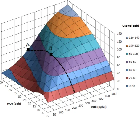
The nonlinear relationship between ozone formed and ini-tial precursors is illustrated using box model simulations in Fig. 1. This figure shows a response surface of daily max-imum 1 h average ozone (ppb) constructed from 121 simu-lations with varying initial NOx(ppb) and VOC (ppbC)

us-ing the 2005 version of the Carbon Bond chemical mech-anism (Yarwood et al., 2005). The ozone response surface is curved throughout indicating that ozone should generally be expected to respond nonlinearly to changes in NOxand/or

VOC. When the ratio of VOC / NOxis high, ozone is reduced

most effectively by reducing NOx(NOx-limited condition).

In contrast, when the ratio of VOC / NOxis low, ozone is

re-duced most effectively by reducing VOC (VOC-limited con-dition).

The line through points A and B in Fig. 1 defines a sec-tion of changing NOx at constant VOC (200 ppbC). If the

derivatives of ozone with respect to NOx(S(1)=∂O3/∂NOx;

S(2)=∂2O3/∂2NOx; etc.) are known, then the response of

ozone to a relative NOx perturbation (1N=1NOx/NOx)

can be approximated using a second-order Taylor series

Fig. 1. Representative response of maximum 1 h average ozone

(ppb) to morning concentrations of emitted NOxand VOC. Section

through points A and B is the ozone response to NOxat constant

VOC of 200 ppbC.

expansion:

1O3(1N )≈1N·S(1)+

1 21N

2_·_S(2)_. ₍₁₎

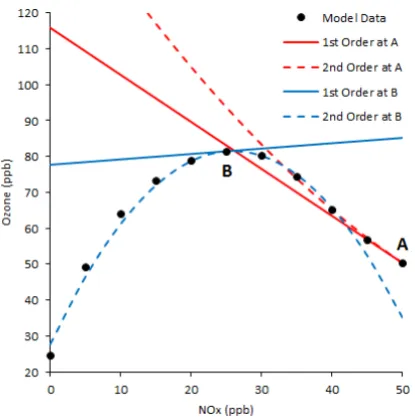
Figure 2 shows the section through points A and B in Fig. 1, including first- and second-order approximations to the ozone response from changing NOxat both A and B

us-ing Eq. (1). The example chosen for Fig. 2 is particularly demanding in selecting a highly curved section of the ozone response surface that traverses a local maximum. This ex-ample shows that for purposes of representing ozone in the range of NOx from zero to A, (1) second-order

representa-tions are generally, but not always, more accurate than first order; (2) second-order representations do not necessarily provide good accuracy (within a factor of two) for response to large perturbations (factor of two change in NOx); and

(3) accuracy is improved by applying Eq. (1) at the center of the range of interest rather than at one extreme. These findings are not surprising but are presented here to explain choices made in this study for applying sensitivity methods to the more complex problem of ozone sensitivity to emis-sions in a 3-D PGM.

2.1 Decoupled direct method

Two widely used methods for computing emissions sensi-tivity within a PGM are the DDM (Dunker, 1981) and the adjoint method (Menut et al., 2000). Both methods can ef-ficiently compute first-order sensitivity coefficients (S(1)=

(3)

G. Yarwood et al.: A method to represent ozone response to large changes in precursor emissions 1603

Fig. 2. Modeled response of ozone to changing NOx at VOC of

200 ppbC. Also shown are first- and second-order Taylor series ap-proximations to the response at points A and B. Points A and B are also marked in Fig. 1.

calculates only first-order sensitivity coefficients (Menut et al., 2000). However, Hakami et al. (2003) demonstrated the application of DDM to second- and third-order sensitivity co-efficients (S(2)=∂2C/∂E2;S(3)=∂3C/∂E3)and called the application high-order DDM (HDDM). The sensitivity coef-ficients needed for this study were computed using HDDM following Dunker et al. (2002) and Cohan et al. (2010).

3 Methods

Modeling was performed with version 5.40 of the Compre-hensive Air quality Model with extensions (CAMx; ENVI-RON, 2012) with model configuration and inputs developed for a previous study of North American background ozone (Emery et al., 2012). Calendar year 2006 was modeled for an outer domain with 36 km grid cells covering the conter-minous US and portions of Canada and Mexico (Fig. 3). Two nested inner domains with 12 km grid cells covered the eastern and western US. The nested 12 km domains commu-nicated with the 36 km grid and with each other by two-way nesting. Meteorological and emissions data were de-veloped by the US EPA for the Air Quality Model Eval-uation International Initiative (AQMEII) program (Rao et al., 2011). Meteorology was modeled using the Weather Re-search and Forecast (WRF) model (Skamarock et al., 2008) at 12 km resolution (Vautard et al., 2012). Emissions data were also at 12 km resolution (Pouliot et al., 2012) and in-cluded the US EPA 2005 national emissions inventory grown to 2006 (EPA, 2010), the Environment Canada 2006 in-ventory (Environment Canada, 2011), a 1999 inin-ventory for

Fig. 3. CAMx North American modeling domain comprised of an

outer 36 km resolution grid and two inner, two-way nested, 12 km resolution grids. The 22 cities used for performance evaluation are marked.

Mexico grown to 2006, biogenic emissions from BEIS ver-sion 3.14 (Vukovich and Pierce, 2002), and fire emisver-sions (Coe-Sullivan, 2008). Chemical boundary conditions for the 36 km grid were down-scaled from 2006 GEOS-Chem ver-sion 8-03-01 global model output (Zhang et al., 2011).

Two annual CAMx simulations were conducted with HDDM to compute ozone sensitivity to US anthropogenic emissions of NOx (N) and VOC (V) at first- and

second-order, yielding sets of 5 ozone sensitivity coefficients from each simulation: S_N(1), S_N(2), S_V(1), S_V(2), S_{N V}(2). Each simula-tion ran for roughly one month using 48 cores on eight Intel X5675 CPUs. The first HDDM simulation computed sensi-tivity coefficients with anthropogenic NOxand VOC

emis-sions reduced to 50 %, corresponding to the example dis-cussed above for point B in Fig. 1. The resulting Taylor series expansion to represent ozone at any NOxand VOC level as

a function of relative changes in NOx(1N=1NOx/NOx)

and VOC (1V =1VOC/VOC) from the 50 % emissions case is

O3(N, V )(50)=O3(50)+1N·S_{N (}(1)₅₀₎+

1 21N

2_·_S(2) N (50)

+1V ·S_{V (}(1)₅₀₎+1

21V

2_·_S(2) V (50)+

1N·1V·S_{N V (}(2) ₅₀₎, (2)

where the subscript “50” indicates a parameter calculated with 50 % anthropogenic emissions. The second HDDM simulation computed sensitivity coefficients with anthro-pogenic NOx and VOC emissions reduced to 10 % in

(4)

emissions level between 0 and 100 % NOxand VOC:

O3(N, V )(10)=O3(10)+1N·S_{N (}(1)₁₀₎+

1 21N

2_·_S(2) N (10)

+1V ·S_{V (}(1)₁₀₎+1

21V

2_·_S(2) V (10)+

1N·1V ·S_{N V (}(2) ₁₀₎, N≤15 %, (3a) O3(N, V )(50)=O3(50)+1N·SN ((1)50)+

1 21N

2_·_S(2) N (50)+

1V·S(_{V (}1)₅₀₎+1

21V

2_·_S(2) V (50)+

1N·1V ·S_{N V (}(2) ₅₀₎, N≥25 %, (3b) O3(N, V )=(N−15)·O3(N, V )(10)

+(25−N )·O3(N, V )(50)

/10,

15< N <25. (3c) Below 15 % NOx (at any VOC) Eq. (3a) is applied

ex-clusively, while above 25 % NOx (at any VOC) Eq. (3b)

is applied exclusively. Within the 15–25 % NOx range (at

any VOC), sensitivity coefficients from both simulations are linearly interpolated across the NOx dimension (N) using

Eq. (3c). The transition points between Eqs. (3a), (3b) and (3c) (i.e., N=15 % andN=25 %) were selected for this application based on results of performance tests with the 3-D PGM, described below. Similarly, defining transition points using N alone performed better than using both N

andV because ozone is predominantly limited by NOx

emis-sions in the 3-D PGM simulations. The transition points for Eqs. (3a)–(3c) could be adjusted for different applications.

Month-long brute force CAMx simulations were per-formed to evaluate the accuracy of Eqs. (2) and (3). Simula-tions were performed for January and July with 100 % NOx

and VOC, 25 % NOx(100 % VOC), and zero NOxand VOC

US anthropogenic emissions. The 100 % and zero anthro-pogenic emission cases bound our range of interest for apply-ing Eqs. (2) and (3). The 25 % anthropogenic NOxemissions

case was useful in developing Eq. (3).

CAMx computes sensitivity coefficients with HDDM for the entire model domain enabling application of Eqs. (2) and (3) at any location within the domain. Results were evalu-ated statistically for all monitoring sites in 22 cities, marked in Fig. 3, by computing the mean bias (MB=P

(HDDM – BF)/n) and mean error (ME=P_|

HDDM−BF|/n) for the n hourly ozone values predicted by the HDDM and brute force (BF) methods. HDDM and BF model results for grid cells containing monitors were paired to calculate the MB and ME statistics.

In addition, results are shown graphically at the locations of an urban and a rural monitor near Dallas, Texas. Dallas was selected because (1) the area is out of compliance with EPA’s ambient ozone standard set at 75 ppb; (2) ozone in Dallas is influenced both by local production and regional transport (Kemball-Cook et al., 2009); and (3) the selected locations exhibit HDDM performance attributes compared to

Fig. 4. Modeled ozone for July 2006 at the urban Dallas location

with 100 % (solid line) and zero (dashed line) US anthropogenic NOxand VOC emissions.

brute force runs that we see in many other areas of the US. The urban location is 1415 Hinton Street, Dallas, in a mixed residential/commercial neighborhood about 1 km from Inter-state Highway 35E and 10 km northwest of central Dallas. The rural location is 3033 New Authon Rd, Weatherford, about 100 km west of central Dallas and 55 km west of Fort Worth. Ozone at the Dallas location is strongly influenced by local emissions and experiences daytime maxima due to pho-tochemical production, and nighttime minima that approach zero due to titration of ozone by local NO emissions. In contrast, the Weatherford location frequently experiences re-gional background ozone except when the urban plume from Dallas/Fort Worth is transported west to the rural monitor lo-cation. Comparisons of HDDM to BF for single sites in Los Angeles and Houston are presented in the Supplement.

4 Results

Figure 4 shows hourly ozone at the Dallas location for the CAMx simulations of July 2006 with 100 % and zero anthro-pogenic NOxand VOC emissions. Relative to background,

anthropogenic emissions alter the entire diurnal distribu-tion of ozone with photochemical ozone producdistribu-tion causing higher daytime maxima and ozone titration by NO causing lower nighttime minima.

Equation (2) was first used to compute January and July hourly ozone at Dallas and Weatherford for both the 100 % and zero anthropogenic emission cases. Equation (2) relies solely upon the ozone concentration and emission sensitivity coefficients computed with 50 % anthropogenic emissions.

(5)

a) January, zero emissions b) January, 100% emissions

c) July, zero emissions d) July, 100% emissions

Fig. 5. Hourly ozone at the urban Dallas location predicted by

HDDM with Eq. (2) vs. brute force CAMx simulations for (a) zero anthropogenic NOxand VOC emissions in January, (b) 100 %

an-thropogenic NOxand VOC emissions in January, (c) zero

anthro-pogenic NOxand VOC emissions in July, and (d) 100 %

anthro-pogenic NOxand VOC emissions in July. Dashed lines show 1:1

agreement and solid red lines show least-squares regressions.

emissions case. The zero anthropogenic emissions case for January (Fig. 5a) has many hours with non-zero brute force ozone (15–35 ppb) but near-zero ozone predicted by Eq. (2) (i.e., points falling below the middle section of the 1:1 line). This type of disagreement occurs for nighttime hours when the CAMx simulation with 50 % anthropogenic emissions had near-zero ozone and consequently had near-zero ozone sensitivity to emissions. For these hours Eq. (2) predicts near-zero ozone at any emission level and so fails to predict that reducing NOxemissions can lead to non-zero ozone at the

point where emitted NO no longer titrates all available ozone. Equation (3) was developed to improve predictions in these hours by incorporating sensitivity coefficients from a CAMx simulation with 10 % anthropogenic emissions that less fre-quently titrate ozone to near zero. The performance of Eq. (3) is discussed below. The July zero anthropogenic emissions case for Dallas (Fig. 5c) has fewer instances of this prob-lem because titration of ozone to near zero is less common in July than in January. The January and July comparisons for the 100 % emissions case (Fig. 5b, d) do not exhibit this problem because when 50 % anthropogenic emissions titrate ozone to near zero, so do 100 % anthropogenic emissions and Eq. (2) predicts accurately. However, the January and July comparisons for the 100 % emissions case show poorer

Fig. 6. Hourly ozone at the urban Dallas location predicted by

HDDM with Eq. (3) vs. brute force CAMx simulations for (a) zero anthropogenic NOxand VOC emissions in January, (b) 100 %

an-thropogenic NOxand VOC emissions in January, (c) zero

anthro-pogenic NOxand VOC emissions in July, and (d) 100 %

anthro-pogenic NOxand VOC emissions in July. Dashed lines show 1:1

agreement and solid red lines show least-squares regressions.

agreement for hours with low ozone (<10 ppb) when Eq. (2) over- or underpredicts the brute force results. These are hours when NOxemissions strongly suppress ozone with 50 %

an-thropogenic emissions causing a strongly nonlinear ozone re-sponse to increasing emissions from 50 to 100 %. Predictions in these hours could be improved by incorporating sensitiv-ity coefficients from a CAMx simulation with near 100 % anthropogenic emissions, although this was not tested.

The improved performance of Eq. (3) over Eq. (2) for the zero anthropogenic emissions case may be seen by compar-ing Figs. 6 and 5 (Fig. 6 repeats Fig. 5 uscompar-ing Eq. 3 in place of Eq. 2). Equation (3) much improves performance for the zero anthropogenic emission cases by incorporating sensitiv-ity coefficients from a CAMx simulation with 10 % anthro-pogenic emissions. There is no change in performance for the 100 % emissions case because Eq. (3b) is equivalent to Eq. (2) for anthropogenic emissions of 25 % and greater.

(6)

Fig. 7. Same as Fig. 5 but for the rural Weatherford location.

agreement with brute force results in all four cases (Fig. 8). Review of results for monitoring sites in other cities (not shown) confirmed that Eqs. (2) and (3) generally perform better at rural than urban sites because ozone is less fre-quently titrated to near zero at rural sites.

a) January, 25% emissions b) July, 25% emissions

Fig. 9. Hourly ozone at the urban Dallas location predicted

by HDDM with Eq. (3) vs. brute force CAMx simulations for

(a) 25 % anthropogenic NOx(100 % VOC) emissions in January,

and (b) 25 % anthropogenic NOx(100 % VOC) emissions in July.

Dashed lines show 1:1 agreement and solid red lines show least-squares regressions.

a) January, 25% emissions b) July, 25% emissions

Equation (3) has transition points at anthropogenic NOx

emission levels of 25 and 15 %. The upper transition point was selected by comparing the accuracy of Eqs. (3a) and (3b) for predicting ozone with 25 % anthropogenic emissions. Equation (3b) was more accurate than Eq. (3a) (Table 1) lead-ing us to rely exclusively on Eq. (3b) for anthropogenic emis-sion levels of 25 % and higher. The lower transition point of 15 % was selected as being between 25 %, where Eq. (3b) proved more accurate, and 10 %, where Eq. (3a) is exact by definition. The transition points in Eq. (3) are a choice that can be refined using brute force results in the region of the transition. Plots showing HDDM vs. BF for the 25 % NOx,

100 % VOC case at Dallas and Weatherford sites are shown in Figs. 9 and 10, respectively (compare to Figs. 6 and 8).

The accuracy of Eq. (3) over 22 cities is summarized in Table 2 for anthropogenic emission levels of 100 % NOxand

VOC, 25 % NOx(100 % VOC), and zero NOxand VOC in

(7)

Table 1. Statistical comparison of two methods for predicting ozone with 25 % anthropogenic NOx(100 % VOC) emissions in 22 cities:

(1) Eq. (3b) based at 50 % emissions versus (2) Eq. (3a) based at 10 % anthropogenic emissions.

Method January 2006 July 2006

Mean Bias Mean Error Mean Bias Mean Error (ppb) (ppb) (ppb) (ppb)

Equation (3b) based at 50 % emissions 0.09 1.27 0.42 0.78 Equation (3a) based at 10 % emissions 1.07 3.89 −7.25 8.69

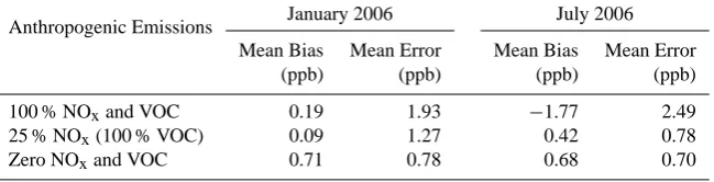
Table 2. Statistical evaluation over 22 cities of using Eq. (3) to predict ozone with 100 % NOxand VOC, 25 % NOx(100 % VOC), and zero

NOxand VOC anthropogenic emissions.

Anthropogenic Emissions January 2006 July 2006 Mean Bias Mean Error Mean Bias Mean Error

(ppb) (ppb) (ppb) (ppb)

100 % NOxand VOC 0.19 1.93 −1.77 2.49

25 % NOx(100 % VOC) 0.09 1.27 0.42 0.78

Zero NOxand VOC 0.71 0.78 0.68 0.70

January, the greatest mean bias and mean error are 0.71 and 1.93 ppb, respectively, whereas in July the greatest mean bias and mean error are−1.77 and 2.49 ppb.

A method similar to Eq. (3) was described recently by Si-mon et al. (2013). Method similarities include use of HDDM to compute second-order sensitivity coefficients and combi-nation of sensitivity coefficients at several emission levels to improve ozone estimation accuracy. A difference is that Eq. (3) uses concentrations derived at two emission levels (10 and 50 % anthropogenic emissions) whereas Simon et al. (2013) use only concentrations derived with 100 % an-thropogenic emissions. Comparing how both methods per-form would be valuable for understanding their respec-tive strengths and limitations and then developing improved methods.

5 Conclusions

This study demonstrates the feasibility of applying HDDM to calculate first- and second-order sensitivity of ozone to anthropogenic NOxand VOC emissions in annual PGM

sim-ulations at continental scale. The resulting sensitivity coeffi-cients are used to construct algebraic models using Taylor se-ries that can accurately represent complete annual frequency distributions of hourly ozone at any location and any anthro-pogenic emission level between zero and 100 %, adjusted in-dependently for NOxand VOC. We recommend computing

the sensitivity coefficients at the midpoint of the emissions range over which they are intended to be applied, in this case with 50 % anthropogenic emissions. The ozone estimates at varying NOxand VOC emissions levels are only valid for the

modeled time period (2006 in this case) and extrapolating

results for 2006 to other years would require additional as-sumptions that are not considered here. The PGM itself has errors associated with inputs, algorithms, discretization, etc., although we note that these types of errors attend all model applications and are not attributable to HDDM.

When ozone predicted by the algebraic model is com-pared to brute force simulations with zero and 100 % anthro-pogenic emissions, the predictions tend to be more accurate in summer than winter, at rural than urban locations, and with 100 % than zero anthropogenic emissions. The photochemi-cal reason for these trends is a strongly nonlinear response of ozone to NOx emissions around the point where NO is

sufficient to titrate ozone to near zero. The algebraic model predictions are improved by incorporating sensitivity coeffi-cients computed with 10 % in addition to 50 % anthropogenic emissions. Equations developed to combine sensitivity coef-ficients computed with 10 and 50 % anthropogenic emissions are able to reproduce brute force simulation results with zero and 100 % anthropogenic emissions with a mean bias of less than 2 ppb and mean error of less than 3 ppb averaged over 22 cities. This approach could be extended by incorporating additional sensitivity coefficients (e.g., computed at or near 100 % anthropogenic emissions) at the cost of greater com-putational expense to obtain the requisite sensitivity coeffi-cients.

(8)

Acknowledgements. The authors acknowledge funding support for

this research from the American Petroleum Institute.

Edited by: A. Lauer

References

Coe-Sullivan, D., Raffuse, S. M., Pryden, D. A., Craig, K. J., Reid, S. B., Wheeler, N. J. M, Chinkin, L. R., Larkin, N. K., Solomon, R., and Strand T.: Development and applications of Systems for Modeling Emissions and Smoke from Fires: The BlueSky Smoke Modeling Framework and SMARTFIRE, Presentation at the EPA 17th Annual International Emission Inventory Conference “In-ventory Evolution – Portal to Improved Air Quality”, Portland, OR, 2–5 June, 2008.

Cohan, D. S., Koo, B., and Yarwood, G.: Influence of uncertain re-action rates on ozone sensitivity to emissions, Atmos. Environ., 44, 3101–3109, 2010.

Dunker, A. M.: Efficient calculation of sensitivity coefficients for complex atmospheric models, Atmos. Environ., Part A, 15, 1155–1161, 1981.

Dunker, A. M., Yarwood, G., Ortmann, J. P., and Wilson, G. M.: The decoupled direct method for sensitivity analysis in a three-dimensional air quality model – Implementation, accuracy, and efficiency, Environ. Sci. Technol., 36, 2965–2976, 2002. Emery, C., Jung, J., Downey, N., Johnson, J., Jimenez, J., Yarwood,

G., and Morris, R.: Regional and global modeling estimates of policy relevant background ozone over the United States, Atmos. Environ., 47, 206–217, doi:10.1016/j.atmosenv.2011.11.012, 2012.

ENVIRON: User’s Guide for the Comprehensive Air Quality Model with Extensions (CAMx), Version 5.4, available at: http://www. camx.com (last access: 30 April 2013), 2012.

Environment Canada: Criteria Air Contaminants web site, avail-able at: http://www.ec.gc.ca/inrp-npri/default.asp?lang=En\&n= 4A577BB9-1 (last access: 17 September 2013), 2011.

EPA: 2005 National Emissions Inventory Data & Documen-tation web site, available at: http://www.epa.gov/ttnchie1/net/ 2005inventory.html (last access: 17 September 2013), 2010. Hakami, A., Odman, M. T., and Russell, A. G: High-order, direct

sensitivity analysis of multidimensional air quality models, Env-iron. Sci. Technol., 37, 2442–2452, 2003.

Kemball-Cook, S., Parrish, D., Ryerson, T., Nopmongcol, U., John-son, J., Tai, E., and Yarwood, G.: Contributions of regional trans-port and local sources to ozone exceedances in Houston and Dallas: Comparison of results from a photochemical grid model to aircraft and surface measurements, J. Geophys. Res., 114, D00F02, doi:10.1029/2008JD010248, 2009.

Menut, L., Vautard, R., Beekmann, M., and Honore, C.: Sensitiv-ity of photochemical pollution using the adjoint of a simpli-fied chemistry-transport model, J. Geophys. Res. Atmos., 105, 15379–15402, 2000.

Pouliot, G., Pierce, T., Denier van der Gon, H., Schaap, M., Moran, M., and Nopmongcol, U.: Comparing emission inventories and model-ready emission datasets between Europe and North Amer-ica for the AQMEII project, Atmos. Environ., 53, 1352–2310, doi:10.1016/j.atmosenv.2011.12.041, 2012.

Rao, S. T., Galmarini, S., and Puckett, K.: Air Quality Model Evaluation International Initiative (AQMEII): advanc-ing state-of-science in regional photochemical modeladvanc-ing and its applications, Bull. Am. Meteorol. Soc., 92, 23–30, doi:10.1175/2010BAMS3069.1, 2011.

Simon, H., Baker, K. R., Akhtar, F., Napelenok, S. L., Possiel, N., Wells, B., and Timin, B.: A Direct sensitivity approach to predict hourly ozone resulting from compliance with the National Ambi-ent Air Quality Standard, Environ. Sci. Technol., 47, 2304–2313, doi:10.1021/es30674e, 2013.

Skamarock, W. C., Klemp, J. B., Dudhia, J., Gill, D. O., Barker, D. M., Duda, M. G., Huang, X.-Y., Wang, W., and Powers, J. G.: A Description of the Advanced Research WRF Version 3, National Center for Atmospheric Research (NCAR), available at: http://www.mmm.ucar.edu/wrf/users/docs/arwv3.pdf (last ac-cess: 17 September 2013), 2008.

US EPA.: Health Risk and Exposure Assessment for Ozone, First External Review Draft (EPA 452/P-12-001, July 2012), http://yosemite.epa.gov/sab/ sabproduct.nsf/db6b9452a00aa3bd85257242006901de/ bace682f1b6d26428525774a0070526e!OpenDocument (last access: 17 September 2013), 2012.

Vautard, R., Moran, M., Solazzo, E., Gilliam, R., Matthias, V., Bian-coni, R., Chemel, C., Ferreira, J., Geyer, B., Hansen, A., Jerice-vic, A., Prank, M., Segers, A., Silver, J., Werhahn, J., Wolke, R., Rao, S. T., and Galmarini, S.: Evaluation of the meteorological forcing used for the Air Quality Model Evaluation International Initiative (AQMEII) air quality simulations, Atmos. Environ., 53, 15–37, doi:10.1016/j.atmosenv.2011.10.065, 2012.

Vukovich, J. M. and Pierce T.: The Implementation of BEIS3 within the SMOKE modeling framework, presentation at the EPA 11th International Emission Inventory Conference – “Emis-sion Inventories – Partnering for the Future”, Atlanta GA, 15–18 April 2002, available at: http://www.epa.gov/ttn/chief/ conference/ei11/modeling/vukovich.pdf (last access: 17 Septem-ber 2013), 2002.

Warneck, P.: Chemistry of the Natural Atmosphere, 2nd Edn., Aca-demic Press, 2000.

Yarwood, G., Rao, S. T., Yocke, M., and Whitten, G. Z.: Up-dates to the Carbon Bond chemical mechanism: CB05, avail-able at: http://www.camx.com/publ/pdfs/CB05_Final_Report_ 120805.pdf (last access: 17 September 2013), 2005.