https://doi.org/10.5194/gmd-11-1497-2018 © Author(s) 2018. This work is distributed under the Creative Commons Attribution 4.0 License.
Implicit–explicit (IMEX) Runge–Kutta methods for
non-hydrostatic atmospheric models
David J. Gardner1, Jorge E. Guerra2, François P. Hamon3, Daniel R. Reynolds4, Paul A. Ullrich2, and Carol S. Woodward1
1Center for Applied Scientific Computing, Lawrence Livermore National Laboratory, 7000 East Ave., Livermore, CA 94550, USA
2Department of Land, Air and Water Resources, University of California, Davis, One Shields Ave., Davis, CA 95616, USA 3Center for Computational Sciences and Engineering, Lawrence Berkeley National Laboratory,
1 Cyclotron Rd., Berkeley, CA 94720
4Department of Mathematics, Southern Methodist University, P.O. Box 750156, Dallas, TX 75257, USA Correspondence:David J. Gardner ([email protected])
Received: 8 November 2017 – Discussion started: 9 November 2017
Revised: 1 February 2018 – Accepted: 2 February 2018 – Published: 17 April 2018
Abstract.The efficient simulation of non-hydrostatic atmo-spheric dynamics requires time integration methods capable of overcoming the explicit stability constraints on time step size arising from acoustic waves. In this work, we investi-gate various implicit–explicit (IMEX) additive Runge–Kutta (ARK) methods for evolving acoustic waves implicitly to en-able larger time step sizes in a global non-hydrostatic atmo-spheric model. The IMEX formulations considered include horizontally explicit – vertically implicit (HEVI) approaches as well as splittings that treat some horizontal dynamics im-plicitly. In each case, the impact of solving nonlinear systems in each implicit ARK stage in a linearly implicit fashion is also explored.
The accuracy and efficiency of the IMEX splittings, ARK methods, and solver options are evaluated on a gravity wave and baroclinic wave test case. HEVI splittings that treat some vertical dynamics explicitly do not show a benefit in solu-tion quality or run time over the most implicit HEVI for-mulation. While splittings that implicitly evolve some hor-izontal dynamics increase the maximum stable step size of a method, the gains are insufficient to overcome the additional cost of solving a globally coupled system. Solving implicit stage systems in a linearly implicit manner limits the solver cost but this is offset by a reduction in step size to achieve the desired accuracy for some methods. Overall, the third-order ARS343 and ARK324 methods performed the best, followed by the second-order ARS232 and ARK232 methods.
1 Introduction
Accurately modeling atmospheric phenomena at horizon-tal resolutions below 10 km necessitates moving to a non-hydrostatic formulation of the governing equations. The step size constraints from sound waves can be addressed either by removing the fast waves in the model with a soundproof for-mulation of the equations or using a numerical method that can stably step over the fastest waves. The latter approach includes split-explicit (e.g., Klemp et al., 2007), implicit– explicit (IMEX) (e.g., Ullrich and Jablonowski, 2012), and fully implicit (e.g., Yang and Cai, 2014; Yang et al., 2016) time stepping methods. Fully implicit methods enable time steps sizes dictated by the timescales of the processes of interest rather than the stability of the fastest propagating waves. However, achieving good scalability with these meth-ods can be quite challenging as they require optimized non-linear solvers and preconditioners to efficiently compute the solution of globally coupled nonlinear systems. As such, split-explicit and IMEX approaches present a potentially simpler alternative as only a subset of the dynamics is treated implicitly. These approaches allow for specialized solvers that can exploit properties of the implicit system at the cost of being stability limited by the fastest waves in the explicit portion of the splitting.
Split-explicit methods typically divide the dynamics into three groups: fast vertical waves that are treated implicitly, fast horizontal waves that are substepped relative to the other dynamics with an explicit method, and slow dynamics that are updated with an explicit method using a long time step (e.g., Klemp et al., 2007). Similarly, IMEX methods parti-tion the dynamics into two parts: non-stiff terms that are ex-plicitly updated and stiff terms that are imex-plicitly solved. In a horizontally explicit – vertically implicit (HEVI) IMEX ap-proach, all horizontal motion is treated explicitly and vertical dynamics are updated implicitly. By solving only the vertical dynamics implicitly, both split-explicit and HEVI methods take advantage of the two-dimensional horizontal domain de-composition of atmospheric models to avoid communication between parallel processes. Since each process owns a sub-set of the vertical columns in the global domain, no message passing is necessary during the vertically implicit solves. Split-explicit approaches are able to gain some additional ef-ficiency by substepping the fast horizontal terms while step sizes with HEVI methods are limited by the fastest horizontal dynamics. This restriction can be overcome by incorporating some horizontal terms into the implicit partition at the cost of solving a larger, globally coupled system requiring inter-processor communication during the implicit solve. If the in-crease in stable step size is sufficiently large, these methods may be able to overcome the additional expense from parallel communication with an efficient nonlinear solver.
With the push toward exascale computing, there has been increasing interest in evaluating the potential of IMEX meth-ods for efficiently simulating atmospheric dynamics at high resolution. Ullrich and Jablonowski (2012) presented re-sults using a Runge–Kutta–Rosenbrock and Strang
carry-over IMEX approach for integrating a non-hydrostatic model in Cartesian geometry. A new second-order Runge–Kutta IMEX method is presented in Giraldo et al. (2013) and compared with Runge–Kutta and multistep IMEX integra-tion schemes from the literature in the non-hydrostatic uni-fied model of the atmosphere (NUMA). Using NUMA, the accuracy and efficiency of the integration methods were evaluated with a one-dimensional linear HEVI splitting and three-dimensional linear IMEX splitting by simulating a two-dimensional rising thermal bubble and inertia–gravity waves in three-dimensional Cartesian and spherical domains. Weller et al. (2013) examined the stability properties of 12 Runge–Kutta IMEX methods and compared the accuracy of the methods with two HEVI splittings against a semi-implicit approach using the two-dimensional compressible Boussi-nesq equations. The work of Lock et al. (2014) performs a detailed analysis of the same IMEX methods from Weller et al. (2013) on linear scalar and two-dimensional wave equa-tions.
In this work, we investigate the performance of 21 Runge– Kutta IMEX methods from the literature, including many of those tested in Ullrich and Jablonowski (2012), Giraldo et al. (2013), Weller et al. (2013), and Lock et al. (2014), on a non-hydrostatic atmospheric dynamical core using dif-ferent implicit–explicit splittings of the governing equations and approaches for solving the nonlinear systems. Methods tested in Weller et al. (2013) and Lock et al. (2014) are evalu-ated with a three-dimensional fully compressible set of gov-erning equations that differs from those considered in Gi-raldo et al. (2013) in terms of formulation, discretization, and approach to implicit–explicit splitting. The Runge–Kutta methods tested in Giraldo et al. (2013) are also included in this study along with additional methods from the literature not considered in the previously cited works. The linearly im-plicit Runge–Kutta–Rosenbrock approach utilized in Ullrich and Jablonowski (2012) is also compared against a Newton iteration for solving the nonlinear systems that arise in each implicit Runge–Kutta stage.
signifi-cant freedom over the choice of methods and implicit solvers. The versions of Tempest with ARKode interfaces used in this work are archived at Gardner et al. (2017).
In the following section, we present the formulation of non-hydrostatic equations implemented in Tempest, fol-lowed by a discussion of the spatial and temporal discretiza-tions and splitting approaches in Sect. 3. The nonlinear and linear solver strategies used with the IMEX methods are cov-ered in Sect. 4. Numerical experiments and the correspond-ing results are given in Sect. 5. A summary of the numerical results, concluding remarks, and directions for future work are given in Sect. 6.
2 Non-hydrostatic equations
The non-hydrostatic dry-atmosphere/shallow-atmosphere equations in the Tempestθ formulation are in terms of co-variant horizontal velocitiesuαanduβ, covariant vertical
ve-locityuξ, potential temperatureθ, and densityρ in an
arbi-trary coordinate system(α, β, ξ ):
∂uα ∂t = −
∂
∂α(K+8)−θ ∂5
∂α (1)
+J uβ(f rξ−1+ζξ)−J uξζβ, ∂uβ
∂t = − ∂
∂β(K+8)−θ ∂5
∂β (2)
−J uα(f rξ−1+ζξ)+J uξζα, ∂uξ
∂t = − ∂
∂ξ(K+8)−θ ∂5
∂ξ +J u
αζβ−uβζα
, (3)
∂θ ∂t = −u
α∂θ ∂α−u
β∂θ ∂β −u
ξ∂θ
∂ξ, (4)
∂ρ ∂t = −
1
J ∂ ∂α Jρu
α−1
J ∂ ∂β Jρu β (5) −1 J ∂ ∂ξ Jρu ξ .
We refer to the system defined by Eqs. (1)–(5) as theθ for-mulation of the non-hydrostatic equations since the thermo-dynamic equation (Eq. 4) is expressed in terms of the poten-tial temperature. The conversion between contravariant and covariant velocity components is given as
ui=giαuα+giβuβ+giξuξ (6)
ui=giαuα+giβuβ+giξuξ, (7)
wheregij andgij are the covariant and contravariant metric
tensors specified in terrain-following Cartesian or spherical coordinates andJ is the metric Jacobian defined as
J =pdetgij. (8)
8 is the product of the gravity constant and elevation r,
rξ=(∂r/∂ξ )is the vertical coordinate transform, andf =
2sinϕ is the Coriolis parameter.K is the specific kinetic energy, defined as
K=1
2 uαu
α+u
βuβ+uξuξ.
and5is the Exner pressure function defined as
5=cp p
0
p
Rd/cp =cp
R dρθ
p0 Rd/cv
,
whereRd,cp, andp0are the gas constant for dry air, specific heat at constant pressure, and the reference pressure (here chosen to be 105Pa), respectively. The relative vorticity vec-tor is
ζ=1 J ∂u ξ ∂β − ∂uβ ∂ξ gα+
∂u α ∂ξ − ∂uξ ∂α
gβ (9)
+ ∂u β ∂α − ∂uα ∂β gξ . 3 Discretization
The non-hydrostatic equations are discretized using a method of lines approach. First, the terms on the right-hand sides of Eqs. (1)–(5) are discretized in space, and then the resulting system of coupled ordinary differential equations is advanced in time with a numerical integration scheme. This two-step process is detailed in the following sections.
3.1 Spatial discretization
The spatial discretization of Eqs. (1)–(5) follows Guerra and Ullrich (2016), where a fourth-order spectral element method is used for horizontal derivatives inα andβ, and the stag-gered finite element method is used inξ. Unless otherwise stated, test cases in this work will be configured with Lorenz vertical staggering (vertical velocity computed and stored at interfaces including model boundaries) and regular grid dis-tribution in each column.
3.2 Temporal discretization
There are numerous approaches for integrating the system of ordinary differentia equations (ODEs) resulting from the spatial discretization of Eqs. (1)–(5), including multistep or multistage methods that treat the system in a fully explicit, fully implicit, or split implicit–explicit manner. This work focuses on the application of multistage IMEX integrators defined by ARK methods that split the right-hand side into two parts: an explicit (non-stiff) and an implicit (stiff) part. Section 3.2.1 presents the general formulation of ARK meth-ods. The various options explored for partitioning terms in the non-hydrostatic equations into implicit and explicit parts are presented in Sect. 3.2.2 and 3.2.3.
3.2.1 Additive Runge–Kutta methods
The spatially discretized non-hydrostatic equations can be written as a general initial value problem with the right-hand side additively split into two parts:
dy dt =f
E(t,y)+fI(t,y), y(t
0)=y0. (10)
The model state vector isy=(uα, uβ, w, θ, ρ)Tin theθ
for-mulation. Under this notation,fEandfIcorrespond to the spatial terms that will be integrated explicitly and implicitly, respectively, and y0 is the initial state at time t0. The sys-tem (Eq. 10) is evolved from timetn−1to timetnusing ARK
methods of the form
zi =yn−1+hn i−1 X
j=1
aEi,jfE(tn,jE ,zj) (11)
+hn i
X
j=1
ai,jI fI(tn,jI ,zj), i=1, . . ., s,
yn=yn−1+hn s
X
i=1
bEifE(tn,iE ,zi)+biIf
I(tI
n,i,zi)
, (12)
whereyn is an approximation of y(tn),zi is an
intermedi-ate stage solution in an ARK method with s stages, hn= tn−tn−1 is the time step size, and tn,iE =tn−1+cEihn and tn,iI =tn−1+cIihnare intermediate stage times. Several of the
methods we examine include an embedded solution,
eyn=yn−1+hn
s
X
i=1
ebEifE(tn,iE ,zi)+ebIifI(tn,iI ,zi), (13)
for estimating the local truncation error to adapt the time step size. The numerical studies that follow use a fixed time step size and thus do not utilize a local error estimate. However, methods with embeddings are of particular interest, as we will explore leveraging variable time step sizes in subsequent work.
A particular ARK method is defined by a combination of an explicit and a diagonally implicit pair of Butcher tableaux:
cE AE bE eb
E
=
0 0 0 0 · · · 0
c2E a2E,1 0 0 · · · 0
c3E a3E,1 a3E,2 0 · · · 0
..
. ... . .. 0
csE aEs,1 as,E2 · · · aEs,s−1 0
bE1 b2E · · · bEs−1 bEs
ebE1 eb2E · · · ebEs−1 ebEs
, (14)
cI AI bI eb
I
=
cI1 a1I,1 0 0 · · · 0
cI2 a2I,1 aI2,2 0 · · · 0
cI3 a3I,1 a3I,2 a3I,3 · · · 0
..
. ... . .. 0
cIs aIs,1 as,I2 · · · as,sI −1 aIs,s bI1 b2I · · · bsI−1 bIs
ebI1 eb2I · · · ebsI−1 ebIs
.
Whenai,iI 6=0, computing the stage valuezi requires
solv-ing a (non)linear system of equations. This system and ap-proaches for computing the stage solutions are discussed in Sect. 4.
While Eqs. (11)–(13) define an ARK method in terms of a linear combination of right-hand side evaluations at inter-nal stage values, we note that it is customary in the climate modeling community to cast ARK schemes as linear com-binations of states produced from explicit and implicit Eu-ler steps. There, the objective is to store state vectors only and make single explicit/implicit function evaluations at a given stage. Since the stage coefficient matrices in Eq. (14) are lower triangular (strictly so for the explicit coefficients), then any preceding function evaluations may be written in terms of preceding state vectors and substituted into a cur-rent stage. While the two approaches are entirely equivalent, we present all ARK methods and their corresponding tables in standard form in Eqs. (11)–(14), both to connect with the literature defining each method, and since we use this form in computing our results.
We investigate a number of ARK methods from the litera-ture with a variety of numerical properties:
– classical second- (ARS232, ARS222, and ARS233) and third-order (ARS343 and ARS443) methods from As-cher et al. (1997);
– the third- (ARK324), fourth- (ARK436), and fifth-order (ARK548) methods from Kennedy and Carpenter (2003);
– the second-order ARK232 method derived for the NUMA model and presented in Giraldo et al. (2013); – second- (SSP2(222), SSP2(332)a, and SSP3(332)) and
– second-order strong stability preserving method SSP2(332)b from Higueras (2006); the opti-mized second-order methods SSP2(332)lpm1, SSP2(332)lpm2, SSP2(332)lpum, and SSP2(332)lspum from Higueras et al. (2014); and the third-order method SSP3(333)a from Higueras (2009); and
– third-order strong stability preserving methods SSP3(333)b and SSP3(333)c from Conde et al. (2017). The ARK232, ARS232, ARS233, ARS443, SSP2(222), SSP2(332)a, SSP3(332), and SSP3(433) methods were pre-viously examined by Weller et al. (2013) with different split-tings on two vertical slice cases of the compressible Boussi-nesq equations. In these tests, the ARK232 method pre-sented in Giraldo et al. (2013) had the best overall perfor-mance. Giraldo et al. (2013) also compared ARK232 with ARK324 and ARK436 with different splittings on a 2-D ris-ing thermal bubble test in Cartesian coordinates and 3-D inertia–gravity wave tests in Cartesian coordinates and on the sphere. The ARK324 and ARK436 methods were most efficient when high accuracy was required and ARK232 had greater efficiency when less accuracy was required. In addi-tion to the methods tested in Weller et al. (2013) and Giraldo et al. (2013), we include the ARS222, ARS343, ARK548, and strong stability preserving (SSP) methods from Higueras (2006), Higueras (2009), Higueras et al. (2014), and Conde et al. (2017).
With the exception of ARS233 and SSP3(333)a, b, and c, all of the above methods are constructed with an L stable implicit method. Thus, the implicit portion of the method is accurate in the limit of the stiff term becoming infinitely fast, meaning that slow dynamics are resolved while fast modes, e.g., acoustic waves, are damped. Two methods, ARS233 and SSP2(222), are B stable which is a nonlinear stability indi-cating that the difference between two numerical solutions does not increase with time. Several methods are SSP and are designed to maintain the total variation diminishing (TVD) property of a spatial discretization. The optimized SSP meth-ods from Higueras et al. (2014) consider additional proper-ties beyond optimizing the region of absolute monotonicity in SSP schemes. A total of 10 of the methods considered are stiffly accurate; that is,as,iI =biI, and two of those meth-ods, ARS222 and ARS443, also haveas,iE =biE. Ascher et al. (1997) notes that having the bothas,iI =bIi andaEs,i=bEi so thatzs =ynis useful for very stiff problems. However, it is
unclear why this property is beneficial and the two methods with this property do not outperform other methods in the two test cases considered. All methods, except ARS222 and ARS443, have the same bi values for the explicit and
im-plicit methods so that thefEandfIfunctions are weighted equally at the same stage solution. As noted in Kennedy and Carpenter (2003) and Giraldo et al. (2013), ARK methods withbE=bI have the desirable property of preserving lin-ear invariants of the problem to machine precision. Many of
the methods considered also have the same explicit and im-plicit stage times. All of the non-SSP methods and the SSP methods of Conde et al. (2017) havecE=cI, but the other SSP methods tested have different explicit and implicit stage times. Finally, the methods of Kennedy and Carpenter (2003) and Giraldo et al. (2013) have implicit methods with second-order stage accuracy to limit second-order reduction when applied to stiff systems. Appendix A contains a summary of different properties of the ARK methods considered in this work. 3.2.2 Horizontally explicit – vertically implicit
splittings
In this section, we present four HEVI formulations of the non-hydrostatic equations (Eqs. 1–5) in which the horizontal terms are evaluated explicitly and some of the vertical terms are solved implicitly. The partitioning of terms into the ex-plicit or imex-plicit right-hand sides is given by
∂uα ∂t = −
∂
∂α(K+8)−θ ∂5
∂α (15)
+J uβ(f rξ−1+ζξ)−J uξζβ, ∂uβ
∂t = − ∂
∂β(K+8)−θ ∂5
∂β (16)
−J uα(f rξ−1+ζξ)+J uξζα, ∂uξ
∂t =−
∂K ∂ξ +u
α∂uα ∂ξ +u
β∂uβ ∂ξ
| {z }
imp (A, C) / exp (B, D)
−∂8 ∂ξ −θ
∂5 ∂ξ
| {z } imp (A, B, C, D)
(17)
−uα∂uξ ∂α −u
β∂uξ ∂β ,
∂θ ∂t = −u
α∂θ ∂α−u
β∂θ
∂β −u
ξ∂θ ∂ξ
| {z } imp (A, B) / exp (C, D)
, (18)
∂ρ ∂t = −
1 J ∂ ∂α Jρu α −1 J ∂ ∂β Jρu β (19) −1 J ∂ ∂ξ Jρu ξ
| {z }
imp (A, B, C, D)
.
The choice of an explicit or implicit treatment of these terms is guided by two core requirements. First, we require that the terms responsible for vertically propagating sound waves (namely, the buoyancy term,−∂8
∂ξ −θ ∂5
∂ξ, in the
ver-tical velocity equation, Eq. 17, and the verver-tical flux term,
−1 J ∂
∂ξ Jρu
ξ
with vertical momentum transport (the first three terms in Eq. 17) must be handled together. In practice, these terms cancel each other nearly exactly and so splitting them can dramatically impact model stability. These terms can be han-dled either implicitly or explicitly, as they are associated with the vertical advective speed, and hence an explicit treatment does not impact model stability. Whereas an explicit treat-ment of these terms is generally simpler, in combination with the last term in Eq. (19) they are together responsible for vertical kinetic energy transport. Consequently, it could be argued that these terms should be handled using the same discretization as the vertical mass transport term in order to ensure energy conservation by the vertically implicit update. In this study, the impact of an explicit and implicit treatment of the vertical transport ofθ is also explored (the last term in Eq. 18). Although sound waves are not expressed in theθ
field, there is a substantial difference in model stability that emerges from whether this term is treated implicitly or ex-plicitly.
Based on the principles above, terms in Eqs. (15)–(19) without underbraces are always evaluated explicitly and those with underbraces are treated either implicitly or explic-itly depending on the particular HEVI formulation. In order from most implicit to least implicit, we consider
1. HEVI-A, where all vertical dynamics except vertical ad-vection of horizontal velocity in Eqs. (15) and (16) are treated implicitly;
2. HEVI-B, where vertical velocity advection in Eq. (17) is treated explicitly;
3. HEVI-C, where thermodynamic advection in Eq. (18) is treated explicitly; and
4. HEVI-D, where vertical velocity advection in Eq. (17) and thermodynamic advection in Eq. (18) are treated ex-plicitly.
3.2.3 IMEX splittings with horizontally implicit terms In addition to the HEVI options, we also consider IMEX splittings that solve various parts of horizontal dynamics plicitly. These formulations contain the same vertically im-plicit terms as HEVI-A but add some of the horizontal terms into the implicit function:
∂uα ∂t = −
∂
∂α(K+8) −θ ∂5
∂α
| {z } imp(B) / exp(A)
(20)
+J uβ(f rξ−1+ζξ)−J uξζβ, ∂uβ
∂t = − ∂
∂β(K+8) −θ ∂5
∂β
| {z } imp(B) / exp(A)
(21)
−J uα(f rξ−1+ζξ)+J uξζα,
∂uξ
∂t =−
∂
∂ξ(K+8)−θ ∂5
∂ξ +u α∂uα
∂ξ +u β∂uβ
∂ξ
| {z }
imp(A, B)
(22)
−uα∂uξ ∂α −u
β∂uξ ∂β ,
∂θ ∂t =−u
α∂θ ∂α−u
β∂θ ∂β
| {z }
imp(B) / exp(A)
−uξ∂θ ∂ξ
| {z } imp , (23) ∂ρ ∂t =− 1 J ∂ ∂α Jρu α −1 J ∂ ∂β Jρu β −1 J ∂ ∂ξ Jρu ξ
| {z }
imp(A, B)
.
(24) As before, terms without underbraces in Eqs. (20)–(24) are treated explicitly. We examine two configurations with hori-zontally implicit terms:
1. IMEX-A, where the density equation (Eq. 24) is fully implicit, and
2. IMEX-B, where the density (Eq. 24), thermodynamics (Eq. 23), and Exner pressure in Eqs. (20) and (21) are solved implicitly.
The IMEX-A option treats the density equation with a sin-gle consistent scheme, while IMEX-B is motivated by semi-implicit splittings (e.g., Weller et al., 2013) and treats the pressure gradient fully implicitly. By incorporating some of the fast horizontal dynamics into the implicit portion of the splitting, these IMEX formulations may enable larger stable step sizes than are possible with the HEVI options. However, treating horizontal dynamics implicitly also introduces cou-pling between vertical columns in the implicit solves, and this increased coupling in turn increases the linear solution expense. In the numerical experiments below, we will test if the increased steps sizes are enough to offset the additional solver cost.
4 Solvers
Ans-stage ARK method defined by Eqs. (11)–(13) requires the solution of at mostsnonlinear systems of the form G(zi)≡zi−hnai,iI fI(tn,iI ,zi)−di=0, i=1, . . ., s, (25)
to compute the stage solutions,zi, where
di≡yn−1+hn i−1 X
j=1 h
ai,jE fE(tn,jE ,zj)+ai,jI f
I(tI
n,j,zj)
i (26)
which determines the size of the system and the spatial cou-pling between the algebraic equations in this system. There-fore, efficient solution strategies that take full advantage of the structure of the nonlinear system resulting from the split-ting are highly desirable. This topic is addressed in the fol-lowing subsections where we present the solver approaches considered in this work.
4.1 Nonlinear solvers
Newton’s method finds the solution of Eq. (25) using an iter-ative approach:
z(mi +1)=zi(m)+δ(m+1), (27) wherem≥0 is the iteration index and the updateδ(m+1) is the solution of the linear system
Az(m)i δ(m+1)= −Gz(m)i , (28) obtained from a linearization of Eq. (25),
Az(m)i ≡I−hnai,iI J
z(m)i , (29)
in whichJis the Jacobian matrix offIevaluated at the cur-rent iteration. Following the ODE literature, we consider the iteration converged when
Rikδ(m+1)k< , (30)
whereRiis an estimate of the linear convergence rate,k·kis a
weighted root mean square (WRMS) norm, andis the non-linear tolerance (Hindmarsh et al., 2005). The convergence rate estimateRi is initialized to 1 and form >0 is updated
as
Ri=max 0.3Ri,
kδ(m+1)k kδ(m)k
!
. (31)
For a vectorvwith lengthN, the WRMS is norm defined as
kvk = 1 N
N
X
i=1
(wivi)2
!1/2
, with wi=
1
r|vi| +a
, (32)
whereaandr are the absolute and relative tolerances for the time-evolved solution, respectively. With this choice of weighting, a WRMS norm of 1 is considered small for any error-like quantities since 1/wi represents a tolerance on the
components of the solution vector. To keep error in the non-linear solve from interfering with the time integration error, we use the ARKode default nonlinear tolerance=10−1in Eq. (30).
Newton’s method can be quite expensive, especially when many iterations are needed to achieve convergence, since each iteration involves computing or approximating the Ja-cobian matrix and performing a linear solve. As an alterna-tive, we also consider treating Eq. (25) as a linearly implicit
system. This Rosenbrock-like approach, used in Ullrich and Jablonowski (2012) and Guerra and Ullrich (2016), consists of performing a single iteration of Newton’s method, thus limiting the cost of the nonlinear solver. However, this ap-proach may produce a lower quality solution when one New-ton iteration does not sufficiently solve the original nonlinear problem.
In both solver approaches, the solution valueyn−1is uti-lized as the initial iterate,z0i (i.e., the trivial predictor) in the nonlinear solves. While alternative predictor methods are not explored in this work, their impact on the speed and robust-ness of the nonlinear solve is a topic of future investigation. 4.2 Linear solvers
Finding the solution of the nonlinear system (Eq. 25) using one or several Newton iterations requires solving the linear system (Eq. 28) for the iteration update. Since the HEVI splittings treat all the horizontal terms explicitly, Eq. (28) does not contain any coupling between the degrees of free-dom in different vertical columns of the atmosphere. That is, the coupling introduced by the implicit terms only acts in the vertical direction, and the linear solve is therefore de-composable into a series of independent column-wise solves. The linear solves in each column are performed with the di-rect banded solverdgbsvfrom the Linear Algebra PACK-age (LAPACK) (Anderson et al., 1999) without any need for interprocessor communication since the domain is par-titioned by vertical columns across parallel processes. More-over, when combined with the Rosenbrock-like approach, no communication is necessary in the nonlinear solve, and nei-ther a nonlinear nor a linear tolerance needs to be set.
The inclusion of horizontal dynamics in the implicit func-tion introduces coupling between degrees of freedom located in different columns, and a linear solve over the full domain is necessary to compute the Newton update. In this case, we employ a Newton–Krylov approach for the nonlinear solve where an approximate solution of Eq. (28) is found using the generalized minimal residual (GMRES) method (Saad and Schultz, 1986). Krylov methods require only the action of a matrix on a vector, and this operation is approximated through a finite difference computation:
Az(m)i v≈
Gz(m)i +σv−Gz(m)i
σ , (33)
residual vectorr satisfies
krk ≤0.1L, (34)
wherek·kis the WRMS norm. Like with the nonlinear solver error, the error in the linear solve must also be controlled to not interfere with the integration error; we therefore utilize the ARKode default value ofL=0.05.
5 Numerical results
We evaluate the accuracy and computational efficiency of the various implicit–explicit splittings, ARK methods, and solver options on two test cases. Section 5.1 presents re-sults for the propagation of gravity waves on a sphere on a reduced-radius planet, and Sect. 5.2 focuses on the devel-opment of a baroclinic wave. Simulations are performed on the Cab Linux computing cluster at Lawrence Livermore Na-tional Laboratory. Each Cab node consists of two Intel Xeon eight-core Sandy Bridge processors with 32 GB of memory per node. All tests are run on six compute nodes using 96 MPI tasks. The absolute and relative tolerances in the numer-ical experiments are a=r=10−4. These tolerances were chosen to produce results with ARKode that matched the so-lutions obtained with the native Tempest implementation of ARS232. The maximum number of Newton iterations is set to 10, and the maximum number of GMRES iterations is set to 50, although these maximum values were only attained in one combination of splitting and solver as noted below. 5.1 Gravity wave
The gravity wave test as defined in Ullrich et al. (2012) be-gins with an initially balanced atmosphere on a reduced-radius Earth (1/125 in size). A small potential temperature perturbation is added to the initial state causing the devel-opment of gravity waves. The domain is discretized using 2400 elements and 10 vertical levels. The test is simulated for 1 h with time steps of 0.01, 0.1, 0.5, 1, 2, 4, and 8 s with each of the different splittings, methods, and solvers de-scribed above. To compare the accuracy and efficiency of the different options, the root mean square error (RMSE) of the state vector with respect to a reference solution is computed at the final time. The reference solution is computed using a step size of 0.001 s with a fully explicit third-order five-stage Runge–Kutta method (KGU35) derived by Ullrich and im-plemented in Tempest (Guerra and Ullrich, 2016). This par-ticular explicit method was created using the stability opti-mization presented in Kinnmark and Gray (1984) to maxi-mize the stability region along the imaginary axis.
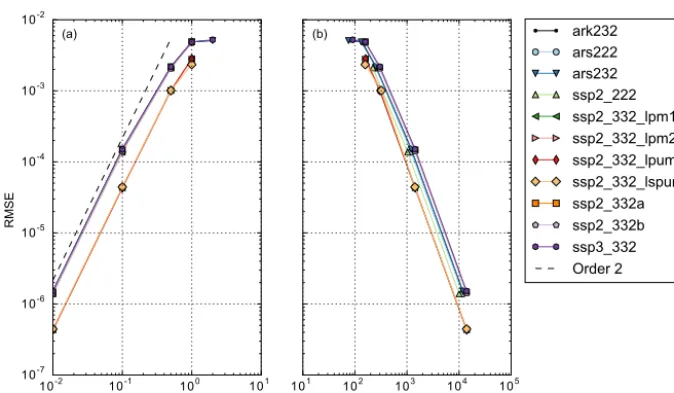
Accuracy and efficiency plots are shown in Figs. 1–6 for the gravity wave test. With the exception of the IMEX-B splitting, as noted below, the choice between a Rosenbrock-like approach or a full Newton iteration to solve the stage systems does not impact the maximum stable time step size
of a given splitting or method, and both solver approaches produce nearly identical errors for this test case. Thus, using only a single Newton iteration provides a sufficiently accu-rate solution to the nonlinear stage systems in each time step. The Newton solver also consistently increases computational cost by approximately 20 to 50 % over the Rosenbrock-like results with HEVI splittings and adds an additional cost of at least 10 % with the IMEX options. Since there is not a signif-icant benefit from a Newton solver in this test case, Figs. 1–6 focus only on results with a Rosenbrock-like approach. The choice of nonlinear solver is more important in the baroclinic wave test case and will be discussed further in the following section. Additionally, treating the vertical velocity or ther-modynamic advection explicitly has a negligible impact on the solution error and integrator efficiency, so results with B, C, and D are indistinguishable from those of HEVI-A. As such, Figs. 1–6 present only HEVI-A, IMEX-A, and IMEX-B results, and any conclusions on the behavior or per-formance of HEVI-A also apply to HEVI-B, C, and D.
The second-order ARK methods can be divided into two groups based on accuracy regardless of the splitting choice. The more accurate group of methods consists of the lpm1, lpm2, lpum, and lspum optimized variants of SSP2(332) from Higueras et al. (2014), and the remaining second-order schemes comprise the second group with slightly less accu-racy.
The approximate largest stable step size is consistent across the HEVI splittings. The ARK232, ARS232, and SSP3(332) methods are stable withhn=2 s, the SSP2(332)
methods are stable with hn=1s , and the remaining two
methods are stable with hn=0.5 s. With the IMEX-A
op-tion, all of the methods are able to achieve a step size of 2 s, and including more implicit terms in IMEX-B increases the maximum step size to 8 s for all of the methods with the Rosenbrock-like approach. The IMEX-B splitting is the only case where integrator behavior differs when using the New-ton solver rather than the Rosenbrock-like approach. In this instance, the maximum stable time step is smaller, approxi-mately one-fourth the step size or smaller depending on the method, with the Newton iteration as it is unable to converge to the given tolerance with larger step sizes. Such behav-ior may be due to using the trivial predictor, and more so-phisticated approaches could improve convergence with the Newton solver. Given the high cost of the IMEX-B splitting with Rosenbrock-like approach compared to the HEVI meth-ods, the evaluation of alternative predictors with the Newton solver is left to future work.
10-2 10-1
100 101
Step size (s) 10-7
10-6 10-5 10-4 10-3 10-2
RMSE
101
102 103 104 105 Run time (s)
Inertia–gravity wave test HEVI-A second-order methods
ark232 ars222 ars232 ssp2_222 ssp2_332_lpm1 ssp2_332_lpm2 ssp2_332_lpum ssp2_332_lspum ssp2_332a ssp2_332b ssp3_332 Order 2
(a) (b)
Figure 1.Accuracy(a)and efficiency(b)for the second-order methods using the Rosenbrock-like approach with the HEVI-A splitting. The dashed line represents second-order convergence. The ARK methods fall into two groups with similar accuracy. Results using multiple New-ton iterations to compute the stage solutions give nearly identical error values to the Rosenbrock-like results but increase the computational cost by 20–50 %.
10-2 10-1 100 101 Step size (s)
10-8 10-7 10-6 10-5 10-4 10-3 10-2
RMSE
101 102 103 104 105 Run time (s)
Inertia–gravity wave test HEVI-A higher-order methods
ark324 ars233 ars343 ars443 ssp3_333a ssp3_333b ssp3_333c ssp3_433 ark436 ark548 Order 3
(a) (b)
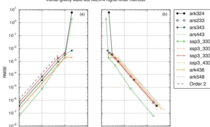
Figure 2.Accuracy(a)and efficiency(b)for the third-, fourth-, and fifth-order methods using the Rosenbrock-like approach with the HEVI-A splitting. The dashed line represents third-order convergence. Results using multiple Newton iterations to compute the stage solutions give nearly identical error values to the Rosenbrock-like results but increase the computational cost by 20–50 %.
with larger error values. Because of the increased stability in the IMEX-A and IMEX-B tests, many of the second-order methods become competitive with the Higueras et al. (2014) SSP2(332) methods athn=2 s, but as with the HEVI
split-tings the optimized SSP2(332) methods are more efficient when greater accuracy is required. Making more terms ex-plicit in the non-hydrostatic equations does not cause a
sig-nificant difference in run times between the HEVI options. The inclusion of horizontally implicit terms and the addi-tional communication necessary in each implicit solve with the IMEX-A and IMEX-B options increases the simulation time by approximately 25–60 % over the HEVI results.
10-2 10-1 100 101 Step size (s)
10-7 10-6 10-5 10-4 10-3 10-2 10-1 100
101
RMSE
102 103 104 105
Run time (s) Inertia–gravity wave test IMEX-A second-order methods
ark232 ars222 ars232 ssp2_222 ssp2_332_lpm1 ssp2_332_lpm2 ssp2_332_lpum ssp2_332_lspum ssp2_332a ssp2_332b ssp3_332 Order 2
(a) (b)
Figure 3.Accuracy(a)and efficiency(b)for the second-order methods using the Rosenbrock-like approach with the IMEX-A splitting. The ARK methods fall into two groups with similar accuracy. The dashed line represents second-order convergence. Results using multiple New-ton iterations to compute the stage solutions give nearly identical error values to the Rosenbrock-like results but increase the computational cost by at least 10 %.
10-2 10-1 100 101 Step size (s)
10-8 10-7 10-6 10-5 10-4
10-3 10-2 10-1 100 101
RMSE
102 103 104 105 Run time (s)
Inertia–gravity wave test IMEX-A higher-order methods
ark324 ars233 ars343 ars443 ssp3_333a ssp3_333b ssp3_333c ssp3_433 ark436 ark548 Order 2
(a) (b)
Figure 4.Accuracy(a)and efficiency(b)for the third-, fourth-, and fifth-order methods using the Rosenbrock-like approach with the IMEX-A splitting. The dashed line represents second-order convergence. Results using multiple Newton iterations to compute the stage solutions give nearly identical error values to the Rosenbrock-like results but increase the computational cost by at least 10 %.
the same level of accuracy, with the exception of SSP3(433), which is generally more accurate, and ARS233, SSP3(333)b, and SSP3(333)c, which are less accurate. The fourth-order accurate ARK436 has smaller errors than all second- and third-order methods, and the fifth-order ARK548 method generally has the lowest error overall. The fifth-order ARK548 does not achieve the expected convergence rate,
10-2 10-1
100 101
Step size (s) 10-7
10-6 10-5 10-4
10-3 10-2 10-1
RMSE
102 103 104
105 Run time (s)
Inertia–gravity wave test IMEX-B second-order methods
ark232 ars222 ars232 ssp2_222 ssp2_332_lpm1 ssp2_332_lpm2 ssp2_332_lpum ssp2_332_lspum ssp2_332a ssp2_332b ssp3_332 Order 2
(a) (b)
Figure 5.Accuracy(a)and efficiency(b)for the second-order methods using the Rosenbrock-like approach with the IMEX-B splitting. The ARK methods fall into two groups with similar accuracy. The dashed line represents second-order convergence. Results using multiple New-ton iterations to compute the stage solutions give nearly identical error values to the Rosenbrock-like results but increase the computational cost by at least 10 %.
10-2 10-1 100 101 Step size (s)
10-8 10-7 10-6 10-5 10-4 10-3 10-2 10-1
RMSE
102 103 104 105 Run time (s)
Inertia–gravity wave test IMEX-B higher-order methods
ark324 ars233 ars343 ars443 ssp3_333a ssp3_333b ssp3_333c ssp3_433 ark436 ark548 Order 3
(a) (b)
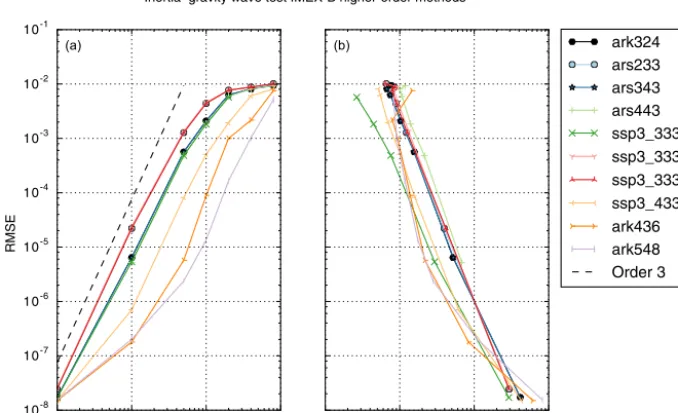
Figure 6.Accuracy(a)and efficiency(b)for the third-, fourth-, and fifth-order methods using the Rosenbrock-like approach with the IMEX-B splitting. The dashed line represents third-order convergence. Results using multiple Newton iterations to compute the stage solutions give nearly identical error values to the Rosenbrock-like results but increase the computational cost by at least 10 %.
components, whereas IMEX-B and HEVI-A treat both terms consistently. As a result, partial derivatives offEandfIin the IMEX-A splitting may have large magnitudes, resulting in increased stiffness, causing the order reduction.
Like the second-order methods, the choice of HEVI splitting does not effect the approximate maximum step size of a given third-order method. ARS233, ARS443, and
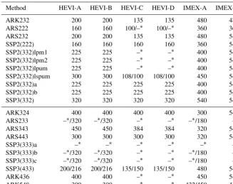
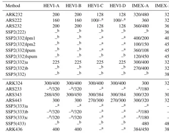
Table 1.Approximate largest stable step size (in seconds) for a 30-day run of the baroclinic wave test. Second-order methods are shown in the top section of the table and higher-order methods in the bottom section. For entries separated by “/”, the left value is the step size for the Rosenbrock-like approach and the right value is the step size for the Newton solver. When a single step size is given, the Rosenbrock-like and Newton solvers were stable at the same step size. As in the gravity wave tests, the choice of a Rosenbrock-like or Newton solver does not generally impact the maximum stable step size, except in the case of IMEX-B which fails to converge. While the methods are able to complete a 30-day run at the step sizes listed below, the solutions produced are not sufficiently accurate in all cases and depend on the solver choice. Table 2 shows the approximate largest step sizes that give acceptable solutions.
Method HEVI-A HEVI-B HEVI-C HEVI-D IMEX-A IMEX-B
ARK232 200 200 135 135 480 480 ARS222 160 160 100/–∗ 100/–∗ 360 360 ARS232 200 200 135 135 480 540 SSP2(222) 160 160 160 160 360 540 SSP2(332)lpm1 225 225 –∗ –∗ 400 540 SSP2(332)lpm2 225 225 –∗ –∗ 400 540 SSP2(332)lpum 225 225 –∗ –∗ 400 540 SSP2(332)lspum 300 300 108/100 108/100 450 540 SSP2(332)a 225 225 225 225 400 540 SSP2(332)b 225 225 225 225 400 540 SSP3(332) 320 320 320 320 540 540
ARK324 400 400 400 400 300 540 ARS233 –∗/320 –∗/320 –∗ –∗ –∗/180 –∗ ARS343 450 450 384 384 320 540 ARS443 300 300 300 300 320 540 SSP3(333)a –∗ –∗ –∗ –∗ –∗ –∗ SSP3(333)b –∗/320 –∗/320 –∗ –∗ –∗/180 –∗ SSP3(333)c –∗/320 –∗/320 –∗ –∗ –∗/180 –∗ SSP3(433) 200/216 200/216 135/150 135/150 480 540 ARK436 400 400 –∗ –∗ 450 540 ARK548 300 300 –∗ –∗ 432/450 432
∗The method was not stable for 30 days withh n≥100s.
in maximum step size to 8 s. As with second-order methods, the IMEX-B splitting is the only option where the choice of a Rosenbrock-like approach alters the integrator results by reducing the maximum step size due to lack of solver con-vergence.
Among the third-order methods, SSP3(443) is the most ef-ficient method, except at the smallest step sizes where con-vergence begins to slow, and SSP3(333)a becomes faster for the same accuracy. Likewise, the fourth- and fifth-order methods are more cost effective until the convergence slows at the smallest time step sizes. SSP3(333)a is the best ap-proach for lower accuracy levels in IMEX-B and is the best scheme in IMEX-A. For higher accuracy with IMEX-B, the faster convergence of ARK436 and ARK548 makes these ap-proaches more efficient until convergence begins to slow at small step sizes. As with the second-order methods, HEVI-B, C, and D do not present an advantage over HEVI-A in run time, and the additional communication required by the hor-izontal terms in the implicit portion of the IMEX methods is not offset by sufficient gains in step size.
With both the second- and higher-order integration meth-ods, HEVI-A with the Rosenbrock-like approach is the best
combination in this test case. For the most part, third-order methods outperform the second-order methods in terms of accuracy at a given step size. Since the third-order meth-ods do not increase the maximum stable step size over that achieved by the second-order methods, the second-order schemes are more efficient at looser error requirements, and higher-order methods are best when more accuracy is neces-sary.
5.2 Baroclinic wave
The second test case simulates the development of a baro-clinic wave over the course of approximately 10 days as de-scribed in Ullrich et al. (2014). For this test case, we focus on how the methods, splittings, and solvers perform near the maximum stable time step size in a 30-day simulation. The domain is discretized with 2400 elements and 30 vertical lev-els. Starting from a step size of 100 s,hnis increased, using
0 5 10 15 20 25 30 Day
0.0 0.2 0.4 0.6 0.8 1.0 1.2 1.4
Max |W|
Baroclinic wave HEVI-A ARS343
450s R 400s R 360s R 320s R 300s R 288s R 450s N
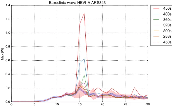
Figure 7.The maximum vertical velocity with ARS343 using the Rosenbrock-like approach (solid lines) and the Newton solver (dashed line) for various time step sizes. The light red region defines the 99 % confidence interval from the explicit simulations with perturbed initial conditions, and the light purple region is 10 % of the maximum deviation in the 99 % confidence interval.
the largest stable step size for a given splitting or method with the exception of six methods (ARS222, SSP2(332)lspum, ARS233, SSP3(333)b, SSP3(333)c, and SSP3(433)). How-ever, the solver selected does affect the quality of the solu-tion produced at large time step sizes, and in many cases a smaller step size may be necessary to compute a sufficiently accurate solution with the Rosenbrock-like approach.
Since this problem produces a strong instability, compar-isons against a highly resolved reference solution, as was used in the gravity wave test, do not yield a good metric for quality of a numerical solution. To define an acceptable nu-merical solution generated by the methods at any given time step, the results of the implicit–explicit simulations (HEVI or IMEX) are compared against the range of maximum vertical velocities produced by five explicit simulations with initial conditions perturbed by random noise. For a state variablex, the perturbed initial value isx=x+max(κ|x|, κ), whereκis a normally distributed random number with mean 0, standard deviationε×1011, andεis machine epsilon. The factor 1011 was selected to produce a max absolute difference (compared to the unperturbed explicit solution) in the vertical veloc-ity after 1 day that is approximately an order of magnitude smaller than the maximum absolute difference observed with the ARS232 scheme using a step size of 200 s. The explicit simulations utilize a Rayleigh sponge layer to damp prob-lematic acoustic transients as, unlike with the ARK meth-ods, there is not an implicit mechanism for dissipating these modes. The sponge layer is 8 km thick with a maximum strength of 0.5 and is applied after the Runge–Kutta (RK) up-date, by way of a backward Euler step, to relax all prognostic fields to the initial state continuously through the depth of the
layer. The explicit simulations are advanced in time with the KGU35 method in Tempest usinghn=2 s which is
nonlin-ear stage systems and yields an acceptable solution with a step size of 450 s. The maximum acceptable time step sizes for the different splittings and integration methods using this methodology for defining an acceptable solution are given in Table 2. The corresponding normalized run times for the step sizes given in Table 2 are listed in Table 3.
Unlike the gravity wave test, treating the thermodynamic advection explicitly (HEVI-C and D) reduces the maximum stable and acceptable step size for some of the integration schemes. As a result, the increased number of time steps with C and D can lead to longer run times than with HEVI-A or B depending on the HEVI-ARK method. Treating only the vertical velocity advection explicitly (HEVI-B) does not im-pact the maximum stable or acceptable step size, nor does it offer a significant advantage in run time over the HEVI-A setup. Handling more terms implicitly in IMEX-A and B can greatly increase the maximum stable step size but, in gen-eral, this does not translate into faster run times due to the in-creased solve cost and the smaller step sizes need to produce a sufficiently accurate solution. However, in a few cases with the Rosenbrock-like approach (ARK232, ARS222, ARS232, SSP2(332)lpm1, and SSP2(332)lpum), IMEX-A runs are faster than results with HEVI-C and D because of the larger acceptable time step size with the IMEX-A splitting and the minimal increase in solver cost due to the effectiveness of the vertical solve as a preconditioner (only two to four linear iter-ations are required per Newton iteration). The preconditioner is less effective in the IMEX-B splitting as more dynamics are included that are not treated by the preconditioner, so 16 to 25 linear iterations are needed per Newton iteration. As in the gravity wave test, the Newton solver does not perform well with the IMEX-B splitting and is unable to converge at step sizes for which the Rosenbrock-like approach gives an acceptable answer.
In this test, the increased accuracy and larger stability re-gions of the higher-order methods enable bigger time step sizes than the second-order methods with HEVI splittings and are somewhat less affected by the choice of HEVI split-ting. The gains in step size are large enough to offset the third implicit stage solve required for ARK324 and ARS343, which consistently perform well. The ARS343 method is the fastest method across the HEVI splittings. ARS233, SSP3(333)b, and SSP3(333)c are less robust to the choice of splitting and solver but, when they produce an accept-able solution (HEVI-A and B with the Newton solver), are the second fastest methods, as they only require two implicit solves per step and have relatively large acceptable step size. ARS324 is more robust to the choice of spitting and solver, and is the third fastest method with HEVI-A and B, and the second fastest method with HEVI-C and D. The second-order ARK232 and ARS232 methods give nearly identical performance and tie for fourth fastest method with the HEVI-A and B splittings.
The ARK324 and ARS343 methods also highlight the po-tential advantage of the Newton solver over the
Rosenbrock-like approach. With the exception of the second-order SSP methods (discussed below), the second-order methods stud-ied produce acceptable solutions at their largest stable step size for HEVI splittings with either a Newton or Rosenbrock-like approach. As a result, there is no benefit from us-ing the Newton solver for second-order methods and the Rosenbrock-like approach is always more efficient. At the larger stable step sizes enabled by higher-order methods, a Rosenbrock-like approach does not always give a sufficiently accurate answer, and a smaller step size is necessary to pro-duce a good solution. Iterating to a converged stage value leads to better results at larger step sizes and, since only a few nonlinear iterations are necessary (on average two itera-tions per stage solve), a HEVI splitting with a Newton solver can outperform the Rosenbrock-like approach when the step size gain is sufficiently large.
While the other higher-order schemes are also able to take larger time steps than the second-order methods, they require more function evaluations or implicit solves than ARK324 or ARS343, and the step size gains are not enough to overcome the additional costs. Four of the third-order methods (ARS233, SSP3(333)b, and SSP3(333)c with the Rosenbrock-like solver, and SSP3(333)a with either solver) are not stable for 30 days at step sizes of at least 100 s with any of the splittings. These failures are likely because the im-plicit parts are not L stable (or even A stable for SSP3(333)a), and the fastest dynamics of the system are not sufficiently damped. These methods did perform well in the gravity wave test case, which might have been due to the reduced domain size altering the eigenvalues of the system.
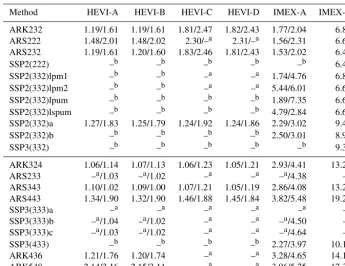
por-Table 2.Approximate largest step size (in seconds) for a 30-day run of the baroclinic wave test that produces acceptable maximum vertical velocities over time. Second-order methods are shown in the top section of the table and higher-order methods in the bottom section. For entries separated by “/”, the left value is the step size for the Rosenbrock-like approach and the right value is the step size for the Newton solver. When a single step size is given, the Rosenbrock-like and Newton solvers gave acceptable solutions at the same step size.
Method HEVI-A HEVI-B HEVI-C HEVI-D IMEX-A IMEX-B
ARK232 200 200 128 128 320/480 320 ARS222 160 160 100/–a 100/–a 360 320 ARS232 200 200 128 128 360/480 360 SSP2(222) –b –b –b –b –b 360 SSP2(332)lpm1 –b –b –a –a 400/200 400 SSP2(332)lpm2 –b –b –a –a 100/150 450 SSP2(332)lpum –b –b –a –a 360/108 450 SSP2(332)lspum –b –b –b –b 120/450 450 SSP2(332)a 225 225 225 225 300/400 320 SSP2(332)b –b –b –b –b 270/400 320 SSP3(332) –b –b –b –b –b 384 ARK324 300/400 300/400 300/400 300/400 300 320 ARS233 –a/320 –a/320 –a –a –a/180 –a ARS343 288/450 300/450 300/384 300/384 300/320 300 ARS443 300 300 270/300 270/300 300/320 320 SSP3(333)a –a –a –a –a –a –a SSP3(333)b –a/320 –a/320 –a –a –a/180 –a SSP3(333)c –a/320 –a/320 –a –a –a/180 –a SSP3(433) –b –b –b –b 480 480 ARK436 400 400 –a –a 384/450 384 ARK548 300 300 –a –a 400/450 384
aThe method was not stable for 30 days withhn≥100s.bThe method was unable to produce an acceptable solution
withhn≥100s.
tion of many of the SSP methods does not include part of the imaginary axis.
6 Conclusions
Considering the results of the gravity wave and baroclinic wave test cases, the HEVI-A and B approaches are the most accurate and efficient of the implicit–explicit splittings con-sidered. Treating some of the vertical dynamics of HEVI-A explicitly does not provide a noticeable gain in efficiency from simpler implicit systems and, in the case of HEVI-C and D, can lead to reduced step sizes in the baroclinic wave test. Adding horizontally implicit terms to the HEVI-A for-mulation does increase the maximum stable step size, but the gains are not large enough to overcome the added cost of a globally implicit solve.
While SSP methods are the most accurate and efficient approaches in the gravity wave test case, they generally do not preform well in the baroclinic wave test (with some no-table exceptions), possibly due to error from the choice of implicit–explicit splitting. The reduced domain size seemed to skew the gravity wave test results in favor of these meth-ods while the other ARK schemes perform well in both test cases. Additionally, the gravity wave test case does not show
a benefit, in terms of maximum stable step size, with higher-order methods, although it does highlight their greater effi-ciency when higher accuracy is required. Again, these re-sults are likely due to the reduced domain size altering the eigenvalues of the system. In the baroclinic wave test on a full-size Earth, higher-order methods produce accurate solu-tions at step sizes large enough to have faster run times than second-order schemes involving fewer implicit solves.
At the larger time step sizes enabled by higher-order methods in the baroclinic wave tests, the choice of non-linear solver approach becomes an important consideration. A Rosenbrock-like approach limits the cost associated with multiple Newton iterations but may require a reduced step size to obtain an accurate solution. Taking larger steps is pos-sible by iterating stage solutions to convergence with New-ton’s method. The additional cost is minimal and can be off-set by the larger step size. The choice of predictor values was not considered in this work but could lead to more effi-cient nonlinear solves with Newton’s method or more accu-rate Rosenbrock-like schemes.
Table 3.The corresponding run times for the approximate largest acceptable step sizes in Table 2. Second-order methods are shown in the top section of the table and higher-order methods in the bottom section. The times have been normalized by the fastest simulation time, HEVI-B using ARS343 with the Newton solver (1372.483 s). The value on the left of the “/” divider is the time for the Rosenbrock-like approach and the value on the right is the time for the Newton solver.
Method HEVI-A HEVI-B HEVI-C HEVI-D IMEX-A IMEX-B
ARK232 1.19/1.61 1.19/1.61 1.81/2.47 1.82/2.43 1.77/2.04 6.84 ARS222 1.48/2.01 1.48/2.02 2.30/–a 2.31/–a 1.56/2.31 6.67 ARS232 1.19/1.61 1.20/1.60 1.83/2.46 1.81/2.43 1.53/2.02 6.49 SSP2(222) –b –b –b –b –b 6.47 SSP2(332)lpm1 –b –b –a –a 1.74/4.76 6.86 SSP2(332)lpm2 –b –b –a –a 5.44/6.01 6.62 SSP2(332)lpum –b –b –b –b 1.89/7.35 6.60 SSP2(332)lspum –b –b –b –b 4.79/2.84 6.69 SSP2(332)a 1.27/1.83 1.25/1.79 1.24/1.92 1.24/1.86 2.29/3.02 9.48 SSP2(332)b –b –b –b –b 2.50/3.01 8.90 SSP3(332) –b –b –b –b –b 9.36 ARK324 1.06/1.14 1.07/1.13 1.06/1.23 1.05/1.21 2.93/4.41 13.28 ARS233 –a/1.03 –a/1.02 –a –a –a/4.38 –a ARS343 1.10/1.02 1.09/1.00 1.07/1.21 1.05/1.19 2.86/4.08 13.21 ARS443 1.34/1.90 1.32/1.90 1.46/1.88 1.45/1.84 3.82/5.48 19.26 SSP3(333)a –a –a –a –a –a –a SSP3(333)b –a/1.04 –a/1.02 –a –a –a/4.50 –a SSP3(333)c –a/1.03 –a/1.02 –a –a –a/4.64 –a SSP3(433) –b –b –b –b 2.27/3.97 10.19 ARK436 1.21/1.76 1.20/1.74 –a –a 3.28/4.65 14.14 ARK548 2.14/3.16 2.15/3.11 –a –a 3.96/5.75 17.31
aThe method was not stable for 30 days withhn≥100s.bThe method was unable to produce an acceptable solution with hn≥100s.
transport as vertical mass transport without a significant dif-ference in computational cost, it is preferred over the HEVI-B option. Overall, the third-order ARS343 method shows excellent performance across the splitting and solver op-tions. ARS233, SSP3(333)b, and SSP3(333)c are also effi-cient third-order methods but their performance depends on the appropriate choice of splitting and solver. A more robust runner-up method is the third-order ARK324 method which follows closely behind ARS343 in run times. The second-order ARS232 and ARK232 methods highlighted in Weller et al. (2013) and Giraldo et al. (2013) using the Rosenbrock-like were also very efficient options.
The ARK324 and ARK232 are of particular interest as both include an embedded method which will be leveraged for future studies on temporal adaptivity in atmospheric sim-ulations using ARKode. Varying the time step size can en-able greater efficiency by placing temporal accuracy where is it needed most to capture dynamics of interest. Addition-ally, we plan on further evaluating the methods in this study on the 2016 dynamical core model intercomparison project (DCMIP2016) test cases to better understand the impacts of coupling with simplified physics on performance of implicit– explicit splittings and integration methods.
Code availability. Tempest is available through the Git repository
Appendix A: ARK method properties
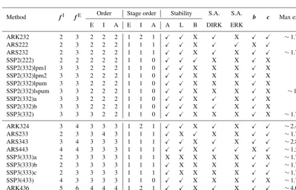
In Table A1, we provide a variety of theoretical properties of each of the ARK methods used in this paper. While we do not reproduce each Butcher table here, references for each method are provided in Sect. 3.2. For each method, we pro-vide the following information:
– number of implicit solves per step (fI column) – the number of nonzero entries on the diagonal ofAI; – number of explicit stages (fEcolumn) – the total
num-ber of RK stages that involve calls tofE;
– order – theoretical order of accuracy of the explicit Runge–Kutta (ERK) method, the diagonally implicit Runge–Kutta (DIRK) method, and the overall ARK method (including coupling conditions);
– stage order – theoretical order of accuracy of stages (relevant for order reduction on stiff problems), again for the ERK stages, DIRK stages, and the overall ARK stages;
– stability – A, L, and B stability for the DIRK portion of each method;
Table A1.Properties for each of the ARK methods used in this paper. The column headings are described in the above text.
Method fI fE Order Stage order Stability S.A. S.A. b c Max exp E I A E I A A L B DIRK ERK
ARK232 2 3 2 2 2 1 2 1 X X X X X X X ∼1.73 ARS222 2 3 2 2 2 1 1 1 X X X X X X X 0 ARS232 2 3 2 2 2 1 1 1 X X X X X X X ∼1.73 SSP2(222) 2 2 2 2 2 1 1 0 X X X X X X X 0 SSP2(332)lpm1 3 3 2 2 2 1 1 0 X X X X X X X 0 SSP2(332)lpm2 3 3 2 2 2 1 1 0 X X X X X X X 0 SSP2(332)lpum 3 3 2 2 2 1 1 0 X X X X X X X 0 SSP2(332)lspum 3 3 2 2 2 1 1 0 X X X X X X X ∼1.2 SSP2(332)a 3 3 2 2 2 1 1 0 X X X X X X X 0 SSP2(332)b 3 3 2 2 2 1 1 0 X X X X X X X 0 SSP3(332) 3 3 3 2 2 1 1 0 X X X X X X X ∼1.73
ARK324 3 4 3 3 3 1 2 1 X X X X X X X ∼2.48 ARS233 2 3 3 4 3 1 1 1 X X X X X X X ∼1.73 ARS343 3 4 3 3 3 1 1 1 X X X X X X X ∼2.83 ARS443 4 4 3 3 3 1 1 1 X X X X X X X ∼1.57 SSP3(333)a 2 3 3 3 3 1 1 1 X X X X X X X ∼1.73 SSP3(333)b 2 3 3 3 3 1 1 1 X X X X X X X ∼1.73 SSP3(333)c 2 3 3 3 3 1 1 1 X X X X X X X ∼1.73 SSP3(433) 4 3 3 3 3 1 1 0 X X X X X X X ∼1.73 ARK436 5 6 4 4 4 1 2 1 X X X X X X X ∼4.00 ARK548 7 8 5 5 5 1 2 1 X X X X X X X ∼0.79
– S.A. DIRK – if the DIRK method is stiffly accurate (i.e., the last row ofAIis the same as thebI);
– S.A. ERK – if the ERK method is “stiffly accurate” (i.e., the last row ofAEis the same as thebE);
– same solution weights (b column) – if the ERK and DIRK methods have the same weights to computeyn (i.e.,bE=bI) and will preserve linear invariants of the problem to machine precision;
– same abscissa (ccolumn) – if the stages in the ERK and DIRK methods are evaluated at the same stage times (i.e.,cE=cI); and
Competing interests. The authors declare that they have no conflict of interest.
Acknowledgements. Support for this work was provided by the
De-partment of Energy, Office of Science Scientific Discovery through Advanced Computing (SciDAC) project “A Non-hydrostatic Variable Resolution Atmospheric Model in ACME”. This work was performed under the auspices of the US Department of Energy by Lawrence Livermore National Laboratory under contract DE-AC52-07NA27344. LLNL-JRNL-737448.
Edited by: Simone Marras
Reviewed by: two anonymous referees
References
Anderson, E., Bai, Z., Bischof, C., Blackford, S., Demmel, J., Don-garra, J., Du Croz, J., Greenbaum, A., Hammarling, S., McKen-ney, A., and Sorensen, D.: LAPACK Users’ Guide, Society for Industrial and Applied Mathematics, 3rd Edn., Philadelphia, PA, 425 pp., 1999.
Ascher, U. M., Ruuth, S. J., and Spiteri, R. J.: Implicit-explicit Runge–Kutta methods for time-dependent partial differential equations, Appl. Numer. Math., 25, 151–167, https://doi.org/10.1016/S0168-9274(97)00056-1, 1997. Conde, S., Gottlieb, S., Grant, Z. J., and Shadid, J. N.: Implicit
and Implicit–Explicit Strong Stability Preserving Runge–Kutta Methods with High Linear Order, J. Sci. Comput., 73, 667–690, https://doi.org/10.1007/s10915-017-0560-2, 2017.
Devore, J. L.: Probability and Statistics for Engineering and the Sci-ences, 7th Edn., Thomson Brooks/Cole, 736 pp., 2008.
Gardner, D. J., Reynolds, D. R., Hamon, F. P., Wood-ward, C. S., Ullrich, P., Guerra, J. E., Lelbach, B. A., and Banide, A. V.: Tempest+ARKode IMEX Tests, https://doi.org/10.5281/zenodo.1162309, 2017.
Giraldo, F. X., Kelly, J. F., and Constantinescu, E. M.: Implicit-Explicit Formulations of a Three-Dimensional Nonhydrostatic Unified Model of the Atmosphere (NUMA), SIAM J. Sci. Comp., 35, B1162–B1194, https://doi.org/10.1137/120876034, 2013.
Guerra, J. E. and Ullrich, P. A.: A high-order staggered finite-element vertical discretization for non-hydrostatic at-mospheric models, Geosci. Model Dev., 9, 2007-2029, https://doi.org/10.5194/gmd-9-2007-2016, 2016.
Higueras, I.: Strong stability for Additive Runge–Kutta methods, SIAM J. Numer. Anal., 44, 1735–1758, https://doi.org/10.1137/040612968, 2006.
Higueras, I.: Characterizing Strong Stability Preserving Addi-tive Runge–Kutta Methods, J. Sci. Comput., 39, 115–128, https://doi.org/10.1007/s10915-008-9252-2, 2009.
Higueras, I., Happenhofer, N., Koch, O., and Kupka, F.: Optimized strong stability preserving IMEX Runge–Kutta methods, J. Com-put. Appl. Math., 272, 116–140, 2014.
Hindmarsh, A. C., Brown, P. N., Grant, K. E., Lee, S. L., Serban, R., Shumaker, D. E., and Woodward, C. S.: SUNDIALS: Suite
of nonlinear and differential/algebraic equation solvers, ACM Trans. Math. Software, 31, 363–396, 2005.
Kennedy, C. A. and Carpenter, M. H.: Additive Runge–Kutta schemes for convection–diffusion–reaction equations, Appl. Numer. Math., 44, 139–181, https://doi.org/10.1016/S0168-9274(02)00138-1, 2003.
Kinnmark, I. P. and Gray, W. G.: One Step Integration Methods of Third–Fourth Order Accuracy with Large Hyperbolic Stability Limits, Mathematics and Computers in Simulation XXVI, 181– 188, 1984.
Klemp, J. B., Skamarock, W. C., and Dudhia, J.: Conservative Split-Explicit Time Integration Methods for the Compressible Nonhydrostatic Equations, Mon. Weather Rev., 135, 2897–2913, https://doi.org/10.1175/MWR3440.1, 2007.
Lock, S.-J., Wood, N., and Weller, H.: Numerical analyses of Runge–Kutta implicit–explicit schemes for horizontally explicit, vertically implicit solutions of atmospheric models, Q. J. Roy. Meteor. Soc., 140, 1654–1669, https://doi.org/10.1002/qj.2246, 2014.
Pareschi, L. and Russo, G.: Implicit-explicit Runge–Kutta schemes and applications to hyperbolic systems with relaxation, J. Sci. Comput., 25, 129–155, https://doi.org/10.1007/BF02728986, 2005.
Reynolds, D. R., Gardner, D. J., Hindmarsh, A. C., Woodward, C. S., and Sexton, J. M.: ARKode – a solver for stiff, nonstiff and mixed systems of ODEs, in preparation, 2018.
Saad, Y. and Schultz, M. H.: GMRES: A generalized minimal resid-ual algorithm for solving nonsymmetric linear systems, SIAM J. Sci. Stat. Comput., 7, 856–869, 1986.
SUNDIALS: SUite of Nonlinear DIfferential/ALgebraic equa-tion Solvers, available at: http://computaequa-tion.llnl.gov/projects/ sundials, 2017.
Taylor, M. A. and Fournier, A.: A compatible and conservative spec-tral element method on unstructured grids, J. Comp. Phys., 229, 5879–5895, 2010.
Ullrich, P. A.: A global finite-element shallow-water model support-ing continuous and discontinuous elements, Geosci. Model Dev., 7, 3017–3035, https://doi.org/10.5194/gmd-7-3017-2014, 2014. Ullrich, P. A. and Jablonowski, C.: Operator-Split Runge–
Kutta–Rosenbrock Methods for Nonhydrostatic Atmo-spheric Models, Mon. Weather Rev., 140, 1257–1284, https://doi.org/10.1175/MWR-D-10-05073.1, 2012.
Ullrich, P. A., Jablonowski, C., Kent, J., Lauritzen, P. H., Nair, R. D., and Taylor, M. A.: Dynamical Core Model In-tercomparison Project (DCMIP) 2012 Test Case Document, v.1.7, available at: https://earthsystemcog.org/site_media/docs/ DCMIP-TestCaseDocument_v1.7.pdf, 2012.
Ullrich, P. A., Melvin, T., Jablonowski, C., and Staniforth, A.: A proposed baroclinic wave test case for deep-and shallow-atmosphere dynamical cores, Q. J. Roy. Meteor. Soc., 140, 1590– 1602, 2014.
Weller, H., Lock, S.-J., and Wood, N.: Runge–Kutta IMEX schemes for the Horizontally Explicit/Vertically Implicit (HEVI) solution of wave equations, J. Comp. Phys., 252, 365–381, https://doi.org/10.1016/j.jcp.2013.06.025, 2013.