Effective Experiment Design and Data Analysis in Transportation Research

(1)

Effective Experiment Design

and Data Analysis in

Transportation Research

NCHRP

_{REPORT 727}

NATIONAL

COOPERATIVE

HIGHWAY

(2)

Chair: Sandra Rosenbloom, Professor of Planning, University of Arizona, Tucson

ViCe Chair: Deborah H. Butler, Executive Vice President, Planning, and CIO, Norfolk Southern Corporation, Norfolk, VA exeCutiVe DireCtor: Robert E. Skinner, Jr., Transportation Research Board

MEMBERS

Victoria A. Arroyo, Executive Director, Georgetown Climate Center, and Visiting Professor, Georgetown University Law Center, Washington, DC J. Barry Barker, Executive Director, Transit Authority of River City, Louisville, KY

William A.V. Clark, Professor of Geography and Professor of Statistics, Department of Geography, University of California, Los Angeles Eugene A. Conti, Jr., Secretary of Transportation, North Carolina DOT, Raleigh

James M. Crites, Executive Vice President of Operations, Dallas-Fort Worth International Airport, TX Paula J. C. Hammond, Secretary, Washington State DOT, Olympia

Michael W. Hancock, Secretary, Kentucky Transportation Cabinet, Frankfort

Chris T. Hendrickson, Duquesne Light Professor of Engineering, Carnegie Mellon University, Pittsburgh, PA Adib K. Kanafani, Professor of the Graduate School, University of California, Berkeley

Gary P. LaGrange, President and CEO, Port of New Orleans, LA Michael P. Lewis, Director, Rhode Island DOT, Providence Susan Martinovich, Director, Nevada DOT, Carson City Joan McDonald, Commissioner, New York State DOT, Albany

Michael R. Morris, Director of Transportation, North Central Texas Council of Governments, Arlington Tracy L. Rosser, Vice President, Regional General Manager, Wal-Mart Stores, Inc., Mandeville, LA Henry G. (Gerry) Schwartz, Jr., Chairman (retired), Jacobs/Sverdrup Civil, Inc., St. Louis, MO

Beverly A. Scott, General Manager and CEO, Metropolitan Atlanta Rapid Transit Authority, Atlanta, GA David Seltzer, Principal, Mercator Advisors LLC, Philadelphia, PA

Kumares C. Sinha, Olson Distinguished Professor of Civil Engineering, Purdue University, West Lafayette, IN Thomas K. Sorel, Commissioner, Minnesota DOT, St. Paul

Daniel Sperling, Professor of Civil Engineering and Environmental Science and Policy; Director, Institute of Transportation Studies; and Acting

Director, Energy Efficiency Center, University of California, Davis

Kirk T. Steudle, Director, Michigan DOT, Lansing

Douglas W. Stotlar, President and CEO, Con-Way, Inc., Ann Arbor, MI

C. Michael Walton, Ernest H. Cockrell Centennial Chair in Engineering, University of Texas, Austin

EX OFFICIO MEMBERS

Rebecca M. Brewster, President and COO, American Transportation Research Institute, Smyrna, GA Anne S. Ferro, Administrator, Federal Motor Carrier Safety Administration, U.S.DOT

LeRoy Gishi, Chief, Division of Transportation, Bureau of Indian Affairs, U.S. Department of the Interior, Washington, DC John T. Gray II, Senior Vice President, Policy and Economics, Association of American Railroads, Washington, DC John C. Horsley, Executive Director, American Association of State Highway and Transportation Officials, Washington, DC Michael P. Huerta, Acting Administrator, Federal Aviation Administration, U.S.DOT

David T. Matsuda, Administrator, Maritime Administration, U.S.DOT

Michael P. Melaniphy, President and CEO, American Public Transportation Association, Washington, DC Victor M. Mendez, Administrator, Federal Highway Administration, U.S.DOT

Tara O’Toole, Under Secretary for Science and Technology, U.S. Department of Homeland Security, Washington, DC

Robert J. Papp (Adm., U.S. Coast Guard), Commandant, U.S. Coast Guard, U.S. Department of Homeland Security, Washington, DC Cynthia L. Quarterman, Administrator, Pipeline and Hazardous Materials Safety Administration, U.S.DOT

Peter M. Rogoff, Administrator, Federal Transit Administration, U.S.DOT

David L. Strickland, Administrator, National Highway Traffic Safety Administration, U.S.DOT Joseph C. Szabo, Administrator, Federal Railroad Administration, U.S.DOT

Polly Trottenberg, Assistant Secretary for Transportation Policy, U.S.DOT

Robert L. Van Antwerp (Lt. Gen., U.S. Army), Chief of Engineers and Commanding General, U.S. Army Corps of Engineers, Washington, DC Barry R. Wallerstein, Executive Officer, South Coast Air Quality Management District, Diamond Bar, CA

Gregory D. Winfree, Acting Administrator, Research and Innovative Technology Administration, U.S.DOT

(3)

NCHRP

REPORT 727

Effective Experiment Design

and Data Analysis in

Transportation Research

Richard W. Lyles M. Abrar Siddiqui

Neeraj Buch William C. Taylor Syed Waqar Haider Dennis C. Gilliland Bruce W. Pigozzi Michigan State UniverSity

East Lansing, Michigan

i n a s s o c i a t i o n w i t h Joseph E. Hummer north carolina State UniverSity

Raleigh, North Carolina

Subscriber Category

Research

T R A N S P O R T A T I O N R E S E A R C H B O A R D

WASHINGTON, D.C.

2012 www.TRB.org

(4)

Systematic, well-designed research provides the most effective approach to the solution of many problems facing highway administrators and engineers. Often, highway problems are of local interest and can best be studied by highway departments individually or in cooperation with their state universities and others. However, the accelerating growth of highway transportation develops increasingly complex problems of wide interest to highway authorities. These problems are best studied through a coordinated program of cooperative research.

In recognition of these needs, the highway administrators of the American Association of State Highway and Transportation Officials initiated in 1962 an objective national highway research program employing modern scientific techniques. This program is supported on a continuing basis by funds from participating member states of the Association and it receives the full cooperation and support of the Federal Highway Administration, United States Department of Transportation.

The Transportation Research Board of the National Academies was requested by the Association to administer the research program because of the Board’s recognized objectivity and understanding of modern research practices. The Board is uniquely suited for this purpose as it maintains an extensive committee structure from which authorities on any highway transportation subject may be drawn; it possesses avenues of communications and cooperation with federal, state and local governmental agencies, universities, and industry; its relationship to the National Research Council is an insurance of objectivity; it maintains a full-time research correlation staff of specialists in highway transportation matters to bring the findings of research directly to those who are in a position to use them.

The program is developed on the basis of research needs identified by chief administrators of the highway and transportation departments and by committees of AASHTO. Each year, specific areas of research needs to be included in the program are proposed to the National Research Council and the Board by the American Association of State Highway and Transportation Officials. Research projects to fulfill these needs are defined by the Board, and qualified research agencies are selected from those that have submitted proposals. Administration and surveillance of research contracts are the responsibilities of the National Research Council and the Transportation Research Board.

The needs for highway research are many, and the National Cooperative Highway Research Program can make significant contributions to the solution of highway transportation problems of mutual concern to many responsible groups. The program, however, is intended to complement rather than to substitute for or duplicate other highway research programs.

Published reports of the

NATIONAL COOPERATIVE HIGHWAY RESEARCH PROGRAM

are available from:

Transportation Research Board Business Office

500 Fifth Street, NW Washington, DC 20001

and can be ordered through the Internet at:

http://www.national-academies.org/trb/bookstore

Printed in the United States of America

Project 20-71 ISSN 0077-5614 ISBN 978-0-309-25849-4

Library of Congress Control Number 2012945556

COPYRIGHT INFORMATION

Authors herein are responsible for the authenticity of their materials and for obtaining written permissions from publishers or persons who own the copyright to any previously published or copyrighted material used herein.

Cooperative Research Programs (CRP) grants permission to reproduce material in this publication for classroom and not-for-profit purposes. Permission is given with the understanding that none of the material will be used to imply TRB, AASHTO, FAA, FHWA, FMCSA, FTA, or Transit Development Corporation endorsement of a particular product, method, or practice. It is expected that those reproducing the material in this document for educational and not-for-profit uses will give appropriate acknowledgment of the source of any reprinted or reproduced material. For other uses of the material, request permission from CRP.

NOTICE

The project that is the subject of this report was a part of the National Cooperative Highway Research Program, conducted by the Transportation Research Board with the approval of the Governing Board of the National Research Council.

The members of the technical panel selected to monitor this project and to review this report were chosen for their special competencies and with regard for appropriate balance. The report was reviewed by the technical panel and accepted for publication according to procedures established and overseen by the Transportation Research Board and approved by the Governing Board of the National Research Council.

The opinions and conclusions expressed or implied in this report are those of the researchers who performed the research and are not necessarily those of the Transportation Research Board, the National Research Council, or the program sponsors.

(5)

government on scientific and technical matters. Dr. Ralph J. Cicerone is president of the National Academy of Sciences.

The National Academy of Engineering was established in 1964, under the charter of the National Academy of Sciences, as a parallel organization of outstanding engineers. It is autonomous in its administration and in the selection of its members, sharing with the National Academy of Sciences the responsibility for advising the federal government. The National Academy of Engineering also sponsors engineering programs aimed at meeting national needs, encourages education and research, and recognizes the superior achievements of engineers. Dr. Charles M. Vest is president of the National Academy of Engineering.

The Institute of Medicine was established in 1970 by the National Academy of Sciences to secure the services of eminent members of appropriate professions in the examination of policy matters pertaining to the health of the public. The Institute acts under the responsibility given to the National Academy of Sciences by its congressional charter to be an adviser to the federal government and, on its own initiative, to identify issues of medical care, research, and education. Dr. Harvey V. Fineberg is president of the Institute of Medicine.

The National Research Council was organized by the National Academy of Sciences in 1916 to associate the broad community of science and technology with the Academy’s purposes of furthering knowledge and advising the federal government. Functioning in accordance with general policies determined by the Academy, the Council has become the principal operating agency of both the National Academy of Sciences and the National Academy of Engineering in providing services to the government, the public, and the scientific and engineering communities. The Council is administered jointly by both Academies and the Institute of Medicine. Dr. Ralph J. Cicerone and Dr. Charles M. Vest are chair and vice chair, respectively, of the National Research Council.

The Transportation Research Board is one of six major divisions of the National Research Council. The mission of the Transporta-tion Research Board is to provide leadership in transportaTransporta-tion innovaTransporta-tion and progress through research and informaTransporta-tion exchange, conducted within a setting that is objective, interdisciplinary, and multimodal. The Board’s varied activities annually engage about 7,000 engineers, scientists, and other transportation researchers and practitioners from the public and private sectors and academia, all of whom contribute their expertise in the public interest. The program is supported by state transportation departments, federal agencies including the component administrations of the U.S. Department of Transportation, and other organizations and individu-als interested in the development of transportation. www.TRB.org

(6)

CRP STAFF FOR NCHRP REPORT 727

Christopher W. Jenks, Director, Cooperative Research Programs Crawford F. Jencks, Deputy Director, Cooperative Research Programs B. Ray Derr, Senior Program Officer

Andréa Harrell, Senior Program Assistant Eileen P. Delaney, Director of Publications Sharon Lamberton, Assistant Editor

NCHRP PROJECT 20-71 PANEL

Field of Special Projects—Area of Research

Donald L. Dean, California DOT, Sacramento, CA (Chair)

Deniz Sandhu, New York State Education Department, formerly New York State DOT, Albany, NY Montasir M. Abbas, Virginia Polytechnic Institute and State University, Blacksburg, VA

Tie He, Nevada DOT (retired), El Dorado Hills, CA

Gary L. Robson, West Virginia DOT (retired), Hurricane, WV Vincent Van Der Hyde, Jr., Oregon DOT (retired), Salem, OR Zhongjie “Doc” Zhang, Louisiana DOTD, Baton Rouge, LA Peter A. Kopac, FHWA Liaison

(7)

This report describes the factors that should be considered in designing experiments and presents 21 typical transportation examples illustrating the experiment design process, including selection of appropriate statistical tests. The examples encompass a wide range of transportation disciplines and statistical methods. This report will be very beneficial to anyone with limited research experience needing to answer a question based on data (e.g., presenting ozone concentrations in a region, determining whether a contractor’s qual-ity assurance/qualqual-ity control procedures are adequate, estimating the effect of automated enforcement on speeds, monitoring trends in the condition of bridge superstructures, devel-oping a user survey to determine the impact of transit fare changes). The report is a com-panion to NCHRP CD-22, Scientific Approaches to Transportation Research, Volumes 1 and 2, which were developed in NCHRP Project 20-45 and present detailed information on statis-tical methods. NCHRP CD-22 is available at http://www.trb.org/Main/Blurbs/152122.aspx

Transportation agencies spend millions of dollars conducting research to improve their ability to plan, design, construct, maintain, and operate the transportation system. These research projects cover a broad range of topics and use approaches ranging from fully con-trolled laboratory experiments to field observational studies. Unfortunately, some research projects use inappropriate experimental designs or data analysis techniques, thereby increas-ing costs and decreasincreas-ing the likelihood of success.

There are many excellent university-level texts on experimental design and data analysis, but these are often not well suited to the needs of those involved in state DOT research. Principal investigators and DOT research program and project managers need practical information that focuses on common problems that DOTs face so that they can make bet-ter decisions when planning and conducting research. NCHRP Project 20-45, “Scientific Approaches for Transportation Research,” produced NCHRP CD-22 that presents valuable material for transportation researchers. It does not, however, cover experimental design.

In NCHRP Project 20-71, Michigan State University and North Carolina State University determined how state DOTs handle experimental design for contract and in-house research and to what extent the results from NCHRP Project 20-45 are in use. They then described basic principles and approaches that should guide experimental design and data analysis in transportation research. Example cases of experiment design were developed across a broad range of functional areas within transportation. The example cases include: (1) the research question being addressed, (2) the dependent and independent variables, (3) data that will be collected, (4) techniques for analyzing the data, (5) interpretation of results, (6) discussion of the process, and (7) application of the approach used in other areas of transportation.

By B. Ray Derr

Staff Officer

(8)

1

Chapter 1 Introduction

1 Developing Effective Experiment Designs and Data Analysis Plans 1 What This Guide Is and Is Not

2 Organization of the Guide

3

Chapter 2 Some Questions and Answers

About Experiment Design

3 What Is the Research Question (What Do You Want to Know)? 5 What Else Needs to Be Asked?

6 What Are Some Typical Problems and Pitfalls? 7 What Factors Affect Outcomes?

9 Summary

10

Chapter 3 Examples of Effective Experiment Design

and Data Analysis in Transportation Research

10 About this Chapter 10 Basic Outline for Examples

11 Techniques Covered in the Examples 12 Areas Covered in the Examples

12 Example 1: Structures/Bridges; Descriptive Statistics 16 Example 2: Public Transport; Descriptive Statistics 19 Example 3: Environment; Descriptive Statistics 23 Example 4: Traffic Operations; Goodness of Fit

26 Example 5: Construction; Simple Comparisons to Specified Values 29 Example 6: Maintenance; Simple Two-Sample Comparisons 31 Example 7: Materials; Simple Two-Sample Comparisons

35 Example 8: Laboratory Testing/Instrumentation; Simple Analysis of Variance (ANOVA)

38 Example 9: Materials; Simple Analysis of Variance (ANOVA) 41 Example 10: Pavements; Simple Analysis of Variance (ANOVA) 44 Example 11: Pavements; Factorial Design (ANOVA Approach) 47 Example 12: Work Zones; Simple Before-and-After Comparisons

50 Example 13: Traffic Safety; Complex Before-and-After Comparisons and Controls 52 Example 14: Work Zones; Trend Analysis

54 Example 15: Structures/Bridges; Trend Analysis

58 Example 16: Transportation Planning; Multiple Regression Analysis 64 Example 17: Traffic Operations; Regression Analysis

66 Example 18: Transportation Planning; Logit and Related Analysis 70 Example 19: Public Transit; Survey Design and Analysis

74 Example 20: Traffic Operations; Simulation

77 Example 21: Traffic Safety; Non-parametric Methods 79 Resources

(9)

1

Introduction

Developing Effective Experiment Designs

and Data Analysis Plans

Personnel in state departments of transportation (DOTs), county road commissions, and other transportation agencies often engage in evaluations of different products or want to know whether a treatment has resulted in an improvement in their system, such as whether some crack sealer is better than the one that was used in the past or whether changing signs on a number of horizontal curves really led to a crash reduction. Some agencies also engage in more comprehen-sive and formal studies through ongoing research programs. The questions asked in informal and formal investigations are significantly different, but the common element is that some sort of experiment design should be done that includes specifying the appropriate statistical analysis. In some cases, the required design and analysis are straightforward; in others, complex. The pur-pose of these guidelines is to help the practitioner ask the right questions and design an analysis that is appropriate to address the research problem.

Throughout NCHRP Report 727, the terms research and experiment design are used fairly loosely. A large, state-funded project undertaken by a local university to evaluate the effectiveness of some statewide highway safety improvement program clearly qualifies as research. In contrast, com-paring the effectiveness of two products that are routinely used may not seem like research that requires a rigorous experiment design. For the purposes of this guide, however, such a comparison is classified as research, and determining the approach to take to make that comparison is, more or less, designing the experiment.

What This Guide Is and Is Not

This guide is not intended to turn practitioners into statisticians. For the expert, let alone the uninitiated, designing experiments and understanding and undertaking complex statistical analysis can be truly daunting. It is unnecessary (and would be ill-advised) to try to turn all traffic engineers, pavement designers, and other transportation researchers into qualified statisticians. However, transportation professionals can learn some of the terminology, understand some of the pitfalls in conducting research, learn to ask effective questions, interact more productively with researchers and statisticians, and obtain understandable and valid test results. Practitioners need to be able to understand what needs to be done and what the results really mean with reference to practice.

(10)

Organization of the Guide

This report has three chapters. Chapter 2 focuses on how to get organized, ask questions, develop an experiment design, and understand how an appropriate statistical technique/ approach is selected. Chapter 3 presents a variety of common examples of experiments in differ-ent areas of interest (e.g., traffic engineering, maintenance, and planning). The examples empha-size working through various questions related to experiment design. The questions lead to the selection of an analysis technique that is appropriate for the research question formulated. The examples are generally short, although some are more in-depth to better illustrate the issues that must be addressed.

(11)

3

Some Questions and Answers

About Experiment Design

This chapter steps the reader through a question-based approach to developing an experi-ment design appropriate for what the potential researcher wants to accomplish. What drives the guidelines is the process of designing an experiment or a research project. This chapter follows a question-and-answer format.

What Is the Research Question

(What Do You Want To Know)?

The first step in designing an experiment or research project, or just undertaking data analysis, is the definition of the problem statement and the objectives of the research. Formulating the right question is important because varying perspectives can lead to different kinds of analysis. Regardless of the quality of the research approach or the qualifications of the analyst, if the wrong question has been asked, the answer may well prove useless. Unfortunately, this happens far more often than people think!

The basic point to be made in formulating effective research questions is that they are rarely as straightforward as they first seem. In real life, the researcher often may be stuck with a less straightforward or more comprehensive question than he or she had hoped for. Under these circumstances, it is important to at least know the limitations of the study (and the eventual conclusions).

The balance of this chapter examines two typical research questions to show how generating and answering additional, related questions help shape the design of the experiment.

Typical Research Question Involving Comparison of Test Results

Is crack sealant A better than crack sealant B? More generally, is one product better than another? This research question can be further generalized to almost any area of transportation where the results of two (or more) treatments, applications, or products need to be compared.

What Does This Question Imply?

(12)

implies is to identify and address related questions. Related questions help to define the breadth of the experiment.

• Does the product have to be better in all situations? The research question “Is crack sealant A better than crack sealant B?” implies that one product or treatment will be selected over another in all cases, which may not be true. In some situations (e.g., when sealing deeper or more numerous cracks), sealant A may outperform sealant B. Under different conditions, sealant B may outperform sealant A.

• If the definition of “better” includes a result that is either difficult to measure or requires a long observation period, can a surrogate measure be used? (Surrogate measures themselves may have problems. If a surrogate measure is considered, it is important to ask how well the surrogate correlates with the real measure.) A classic example of using a surrogate measure in traffic safety research involves evaluation of crash frequencies and rates, which are the ultimate measures of safety but can require an experiment time frame that covers many years. Some researchers/ engineers use traffic conflicts (e.g., near-misses in which one vehicle must unexpectedly give way to another) as a surrogate for crashes. Traffic conflicts provide a reasonably effective surrogate measure for crash frequencies because measuring the near-misses allows researchers to compile a larger sample of data within a shorter period of time.

• How large must the sample be to determine whether one product is better than another? The answer to this question involves confidence limits, the cost of obtaining samples of the vari-ous products being evaluated, and the potential dollar savings associated with choosing one product over the other under various experimental conditions.

• Are there other consequences of using one product over the other? These could include, for example, the cost of application, environmental costs, and potential long-term price changes for the product.

Typical Research Question Involving Independent and Dependent Variables

What is the effect of increasing truck traffic on ride quality? More generally, does variation in one variable (e.g., truck volume) affect the outcome or value of some other variable (e.g., ride quality)?

What Does This Question Imply?

Answering this question involves determining correlation or calibrating an equation where a dependent variable is a function of one or more independent variables. Addressing a question like this typically involves obtaining data and then fitting an equation to the data (e.g., using linear or non-linear regression). It is important to be clear whether changes in the independent variable (truck traffic) really have a causal impact on the dependent variable (ride quality).

What Issues Must Be Considered?

• Does the relationship involve cause and effect? One of the most fundamental (and critical) issues that must be considered with research involving variables is whether observed correla-tions indicate causal relacorrela-tionships. Although establishing correlation is necessary for causa-tion, it is not sufficient. That is, even when correlation can be measured, this may not mean that a cause-and-effect relationship exists. This is a fundamental question to consider when causal models are desired.

(13)

• Do other variables also have an impact on ride quality? If so, how can the effects of one vari-able be separated from the effects of others?

• Is the conclusion true in all cases? In this example, does the relationship between truck volume and ride quality hold for all pavement types over the entire range of truck volumes and for all types of trucks?

• What is the form of the relationship between the dependent and independent variables? Sta-tistically, is the form of the relationship linear throughout, non-linear throughout, or does it vary across the observed range of values (e.g., it is linear for low values of the independent variables and non-linear for higher values)?

• Based on the nature of the phenomenon, is it necessary that the fitted regression line pass through the origin (where both the dependent and independent variables equal zero)? If not, what is the meaning of the intercept?

• What statistics are appropriate for evaluating the regression line? What are the effects of outliers in the data set?

What Else Needs to Be Asked?

Anyone undertaking or supervising a study or research project (no matter how big or small) might need to know many other things. It’s hard to make a comprehensive list, especially because not everyone is faced with the same situations. That said, some additional questions follow that might be useful to think about.

Why Do a Statistical Analysis?

This question has probably been around as long as researchers have been trying to answer questions about whether some action (or project) is worthwhile, or whether some procedure or product should be changed. Often, research is conducted simply to gain more confidence in decisions that have already been made.

In general, statistical analysis is used to try to explain an observed variation (e.g., varia-tion in pavement roughness, the number of vehicle crashes on curved roadway secvaria-tions, or the performance of a product like a crack sealant). Statistical analysis can help clarify the relationship between these observations and variations in pavement design, the degree of curvature of the road, or the material differences in sealants. Although these might not be the only variables that should be considered, the idea is to use statistics to examine what it is that explains the variations that have been observed.

How Much Data Must Be Collected?

This age-old question can also be put another way: What size does the sample size need to be? The answer relates to the variation the research seeks to explain. Let’s say a researcher wants to estimate a mean or average value of something (x). If all observations of x result in the same value, then there is no variance. The average value is the same as any single observation. If there is no variance, then a single observation—a sample size of one—will establish the “truth.”

(14)

When determining sample size, it is also important to consider the amount of difference in the results that is important for the decision the experiment is designed to support. The more preci-sion the researcher is looking for in an answer, the more data must be collected. For example, is it important to know whether increased police presence in a work zone reduces the average speed of traffic by 1 mile per hour, or would the researchers recommend using increased enforcement only if it resulted in a reduction of 5 miles per hour or more?

Because the cost of data collection often is a function of the number of observations collected, an understanding of the required accuracy is important.

If a researcher expects estimates or answers to vary according to specific parameters, the researcher needs to consider these variations in the experiment design and the sample size cal-culations. For example, a researcher might study pavement behavior in a state such as Michigan, which encompasses two distinct freeze-thaw zones. The researcher will need an appropriate sample size in each of the freeze-thaw zones to make conclusions that are applicable statewide. The analysis will also need to consider the amount of the overall variance in pavement behavior that is attributable to differences in freeze-thaw zones.

Does the Type of Data Collected Make a Difference?

The term type can be interpreted in several ways, but in statistical analysis the researcher is concerned with what form the data takes. Is the variable that is being measured continuous or discrete? The type of data often determines the kind of analysis that can be done. For example, although exceptions occur, linear regression typically requires that both dependent and inde-pendent variables be continuous (or that they can be assumed to be continuous). On the other hand, simple analysis of variance (ANOVA) techniques work when the dependent variable is continuous and the independent variables are discrete/categorical. (Different types of data and the implications for selection of analysis techniques are comprehensively discussed in NCHRP Project 20-45, Volume 2, Chapter 1, “Identification of Empirical Setting.”)

What Are Some Typical Problems and Pitfalls?

Even after researchers and their collaborators come to agreement on the basic research ques-tion, issues may still be encountered. Understanding the typical problems and pitfalls can help practitioners avoid or address them proactively, before they can jeopardize the usefulness of research results.

Is the Research Question Misleading, Too Simple, or Wrong?

Some questions are either wrong or lead to incomplete or poor experiments. For example, the sample question about the relationship between truck traffic and ride quality is fairly simple. The implicit assumption is that truck traffic is the major (or perhaps the only) determinant of ride qual-ity; however, other factors could easily have an impact on ride quality. It might be interesting to know the extent to which ride quality degradation is related to truck traffic, but determining whether truck traffic can be effectively controlled is problematic. This might be a valid question to ask in relation to local streets and roads (where truck access can be controlled), but it may not be valid for the interstate/freeway system (where there is generally less control).

(15)

espe-cially within a limited budget. The following questions can help transportation professionals determine whether a research question is misleading, too simple, or wrong.

Has the Question Already Been Answered?

In these days of burgeoning information, it is sometimes hard to believe that any questions exist that haven’t already been addressed. It is fundamental to determine whether the research project that is envisioned has already been done, and if so whether all the questions have been answered.

If the questions really have been answered, the solution is straightforward—don’t do the proj-ect. Often, however, researchers find a question has been asked and answered “somewhere else” (i.e., in a different state or region of the country). In such instances, it may still be reasonable to conduct a similar study to make sure that results are consistent in the local environment. For example, in traffic safety it is well known that driving styles differ from place to place and the results of very similar studies are not necessarily consistent. The clear implication here is that the literature should be critically reviewed. The experiment design should be carefully crafted so that results can be compared (to the extent possible) to those from other projects and locations. Indeed, the experiment design used for a past project may be appropriate for a new project with very little change.

Does Real Disagreement Exist About the Question/Issue?

As with the previous issue, sometimes there is simply no good reason to undertake the research. A product or a technique may have been tested so often that everyone knows the answer. In such cases, although there is no need to reinvent the wheel, another level of analysis might be appro-priate (i.e., a meta-analysis constructed to consider the results of a variety of similar studies). If a meta-analysis seems warranted, it is advisable to consult with a professional statistician.

If little or no disagreement exists about a question or issue, the most obvious outcome is to question whether the study really needs to be done. In general, research money seems too scarce these days to waste dollars on studies that really don’t extend the state of the art.

What Factors Affect Outcomes?

Once the researcher is satisfied that he or she is asking the right research question and is comfortable with its form, the next step is to determine whether other factors may affect or complicate the answer.

There are almost always some other factors that can affect the outcome of a research proj-ect. Some factors may be unexpected while others may simply be overlooked. For example, if researchers want to look at the total crashes that occurred at a set of intersections after changing them in some way, the crash frequency might have been affected by an exceptionally hard winter that resulted in many more “icy road” crashes or by the fact that some of the intersections are on a road that served as a detour for another road that was closed for the construction season, thus causing significant changes in traffic volume through the studied site. Another example might be a longer study on the performance of pavements during which the volume of trucks on the road being studied unexpectedly increases (or decreases) because of detours, construction, changes in land use, or any of several other reasons.

In general, researchers have two choices for dealing with such problems:

(16)

2. They can explicitly consider the variations due to other factors in the selection of their analy-sis approach.

At this point, it is sufficient to answer the following questions. The answers to these questions also help determine which data need to be collected.

What Other Factors Can Affect the Answers to Your Research Question?

In the crack sealant example, both the average size of the cracks and the ambient temperature when the sealant was applied might affect the performance of either crack sealant A or crack sealant B in any individual application. This question reveals that there are other effects that the researcher needs to track in addition to measuring the basic performance of the sealant. The experiment design and the analysis approach need to be planned in a way that explicitly considers these other effects.

Can the Experiment Be Designed to Control for the Variations Caused by Other Factors?

For example, a researcher interested in measuring the ride quality of alternative pavement designs over time might consider how to take into account the effects of truck traffic. This ques-tion implies that the researcher must either isolate the effects being studied (e.g., by selecting sites with similar truck volumes) or explicitly control for other factors in the analysis (e.g., by using control sites or certain kinds of statistical techniques).

Can Site Selection Affect Results? How Can the Researcher Determine the Suitability of a Site for Collecting Data?

This question implies that researchers must also consider the impact that a site might have on the ultimate analysis and the results of the analysis. The effects of site selection can be handled in a couple of ways. First, researchers can control for the impacts of a site just like any other independent variable. This is typically done to determine whether results obtained from one site are unique or consistent with those obtained at similar sites. For most projects, desir-able sites will be similar enough to be effectively interchangedesir-able. This is especially true if the researcher is treating some sites and using others as untreated controls for comparison pur-poses. To select appropriate sites, the researcher needs to compile the characteristics that may impact the experiment and then select sites that are similar when compared on the basis of those characteristics. For example, for a traffic safety-related project or experiment in which average vehicle speed is an important measure of effectiveness, important site selection criteria would include characteristics of traffic flow such as the speed limit, the truck percentage (or volume), and the grade of the roadway.

What Are Independent Samples? How Might They Affect Results?

For most research projects, it is important that the data collected be both representative and

independent. For example, in a study of pavement characteristics using sample cores in a mile-long

(17)

In this experiment, researchers might want to collect data about vehicle speeds at, say, the point of curvature (after the motorist has seen and responded to the device). It would be important to collect only the speeds of free-flowing (lead) vehicles, disregarding those vehicles following in a line and vehicles completely separated from other vehicles (e.g., following more than X seconds behind a preceding vehicle). The researcher wants to collect the speeds of vehicles whose drivers are affected only by the signs themselves and whose actions are independent of the actions of the drivers in vehicles that precede them.

Summary

(18)

10

Examples of Effective Experiment

Design and Data Analysis in

Transportation Research

About this Chapter

This chapter provides a wide variety of examples of research questions. The examples demon-strate varying levels of detail with regard to experiment designs and the statistical analyses required. The number and types of examples were selected after consulting with many practitioners. The attempt was made to provide a couple of detailed examples in each of several areas of transporta-tion practice. For each type of problem or analysis, some comments also appear about research topics in other areas that might be addressed using the same approach. Questions that were briefly introduced in Chapter 2 are addressed in considerably more depth in the context of these examples.

All the examples are organized and presented using the outline below. Where applicable, ref-erences to the two-volume primer produced under NCHRP Project 20-45 have been provided to encourage the reader to obtain more detail about calculation techniques and more technical discussion of issues.

Basic Outline for Examples

The numbered outline below is the model for the structure of all of the examples that follow.

1. Research Question/Problem Statement: A simple statement of the research question is

given. For example, in the maintenance category, does crack sealant A perform better than crack sealant B?

2. Identification and Description of Variables: The dependent and independent variables

are identified and described. The latter includes an indication of whether, for example, the variables are discrete or continuous.

3. Data Collection: A hypothetical scenario is presented to describe how, where, and when

data should be collected. As appropriate, reference is made to conventions or requirements for some types of data (e.g., if delay times at an intersection are being calculated before and after some treatment, the data collected need to be consistent with the requirements in the

Highway Capacity Manual). Typical problems are addressed, such as sample size, the need

for control groups, and so forth.

4. Specification of Analysis Technique and Data Analysis: The links between successfully

framing the research question, fully describing the variables that need to be considered, and the specification of the appropriate analysis technique are highlighted in each example. Refer-ences to NCHRP Project 20-45 are provided for additional detail. The appropriate types of statistical test(s) are described for the specific example.

5. Interpreting the Results: In each example, results that can be expected from the analysis are

(19)

a comparison of means indicates whether the mean values of two distributions can be con-sidered to be equal with a specified degree of confidence) as well as an operational perspective (e.g., judging whether the difference is large enough to make an operational difference). In each example, the typical results and their limitations are discussed.

6. Conclusion and Discussion: This section recaps how the early steps in the process lead

directly to the later ones. Comments are made regarding how changes in the early steps can affect not only the results of the analysis but also the appropriateness of the approach.

7. Applications in Other Areas of Transportation Research: Each example includes a short list

of typical applications in other areas of transportation research for which the approach or analysis technique would be appropriate.

Techniques Covered in the Examples

The determination of what kinds of statistical techniques to include in the examples was made after consulting with a variety of professionals and examining responses to a survey of research-oriented practitioners. The examples are not exhaustive insofar as not every type of statistical analysis is covered. However, the attempt has been made to cover a representative sample of tech-niques that the practitioner is most likely to encounter in undertaking or supervising research-oriented projects. The following techniques are introduced in one or more examples:

• Descriptive statistics

• Fitting distributions/goodness of fit (used in one example)

• Simple one- and two-sample comparison of means

• Simple comparisons of multiple means using analysis of variance (ANOVA)

• Factorial designs (also ANOVA)

• Simple comparisons of means before and after some treatment

• Complex before-and-after comparisons involving control groups

• Trend analysis

• Regression

• Logit analysis (used in one example)

• Survey design and analysis

• Simulation

• Non-parametric methods (used in one example)

Although the attempt has been made to make the examples as readable as possible, some tech-nical terms may be unfamiliar to some readers. Detailed definitions for most applicable statistical terms are available in the glossary in NCHRP Project 20-45, Volume 2, Appendix A. Most defini-tions used here are consistent with those contained in NCHRP Project 20-45, which contains useful information for everyone from the beginning researcher to the most accomplished statistician.

Some variations appear in the notations used in the examples. For example, in statistical analy-sis an alternate hypotheanaly-sis may be represented by Ha or by H1, and readers will find both notations

used in this report. The examples were developed by several authors with differing backgrounds, and latitude was deliberately given to the authors to use the notations with which they are most familiar. The variations have been included purposefully to acquaint readers with the fact that the same concepts (e.g., something as simple as a mean value) may be noted in various ways by different authors or analysts.

(20)

Areas Covered in the Examples

Transportation research is very broad, encompassing many fields. Based on consultation with many research-oriented professionals and a survey of practitioners, key areas of research were identified. Although these areas have lots of overlap, explicit examples in the following areas are included:

• Construction

• Environment

• Lab testing and instrumentation

• Maintenance

• Materials

• Pavements

• Public transportation

• Structures/bridges

• Traffic operations

• Traffic safety

• Transportation planning

• Work zones

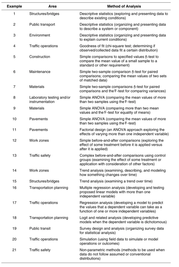
The 21 examples provided on the following pages begin with the most straightforward ana-lytical approaches (i.e., descriptive statistics) and progress to more sophisticated approaches. Table 1 lists the examples along with the area of research and method of analysis for each example.

Example 1: Structures/Bridges; Descriptive Statistics

Area: Structures/bridges

Method of Analysis: Descriptive statistics (exploring and presenting data to describe existing

conditions and develop a basis for further analysis)

1. Research Question/Problem Statement: An engineer for a state agency wants to determine

the functional and structural condition of a select number of highway bridges located across the state. Data are obtained for 100 bridges scheduled for routine inspection. The data will be used to develop bridge rehabilitation and/or replacement programs. The objective of this analysis is to provide an overview of the bridge conditions, and to present various methods to display the data in a concise and meaningful manner.

Question/Issue

Use collected data to describe existing conditions and prepare for future analysis. In this case, bridge inspection data from the state are to be studied and summarized.

2. Identification and Description of Variables: Bridge inspection generally entails collection of

(21)

Example Area Method of Analysis

1 Structures/bridges Descriptive statistics (exploring and presenting data to describe existing conditions)

2 Public transport Descriptive statistics (organizing and presenting data to describe a system or component)

3 Environment Descriptive statistics (organizing and presenting data to explain current conditions)

4 Traffic operations Goodness of fit (chi-square test; determining if observed/collected data fit a certain distribution) 5 Construction Simple comparisons to specified values (t-test to

compare the mean value of a small sample to a standard or other requirement)

6 Maintenance Simple two-sample comparison (t-test for paired comparisons; comparing the mean values of two sets of matched data)

7 Materials Simple two-sample comparisons (t-test for paired comparisons and the F-test for comparing variances) 8 Laboratory testing and/or

instrumentation Simple ANOVA (comparing the mean values of more than two samples using the F-test)

9 Materials Simple ANOVA (comparing more than two mean

values and the F-test for equality of means)

10 Pavements Simple ANOVA (comparing the mean values of more

than two samples using the F-test)

11 Pavements Factorial design (an ANOVA approach exploring the effects of varying more than one independent variable) 12 Work zones Simple before-and-after comparisons (exploring the

effect of some treatment before it is applied versus after it is applied)

13 Traffic safety Complex before-and-after comparisons using control groups (examining the effect of some treatment or application with consideration of other factors) 14 Work zones Trend analysis (examining, describing, and modeling

how something changes over time)

15 Structures/bridges Trend analysis (examining a trend over time) 16 Transportation planning Multiple regression analysis (developing and testing

proposed linear models with more than one independent variable)

17 Traffic operations Regression analysis (developing a model to predict the values that a dependent variable can take as a function of one or more independent variables) 18 Transportation planning Logit and related analysis (developing predictive

models when the dependent variable is dichotomous) 19 Public transit Survey design and analysis (organizing survey data

for statistical analysis)

20 Traffic operations Simulation (using field data to simulate or model operations or outcomes)

21 Traffic safety Non-parametric methods (methods to be used when data do not follow assumed or conventional distributions)

(22)

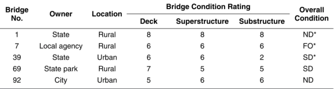
3. Data Collection: Data are collected at 100 scheduled locations by bridge inspectors. It is

important to note that the bridge condition rating scale is based on subjective categories, and there may be inherent variability among inspectors in their assignment of ratings to bridge components. A sample of data is compiled to document the bridge condition rating of the three primary structural components and the overall condition by location and ownership (Table 2). Notice that the overall condition of a bridge is not necessarily based only on the condition rating of its components (e.g., they cannot just be added).

4. Specification of Analysis Technique and Data Analysis: The two primary variables of

inter-est are bridge condition rating and overall condition. The overall condition of the bridge is a categorical variable with three possible values: not deficient; structurally deficient; and functionally obsolete. The frequencies of these values in the given data set are calculated and displayed in the pie chart below. A pie chart provides a visualization of the relative proportions of bridges falling into each category that is often easier to communicate to the reader than a table showing the same information (Figure 1).

Another way to look at the overall bridge condition variable is by cross-tabulation of the three condition categories with the two location categories (urban and rural), as shown in Table 3. A cross-tabulation provides the joint distribution of two (or more) variables such that each cell represents the frequency of occurrence of a specific combination of pos-sible values. For example, as seen in Table 3, there are 10 structurally deficient bridges in rural areas, which represent 11.4% of all rural area bridges inspected. The numbers in the parentheses are column percentages and add up to 100%. Table 3 also shows that 88 of the bridges inspected were located in rural areas, whereas 12 were located in urban areas.

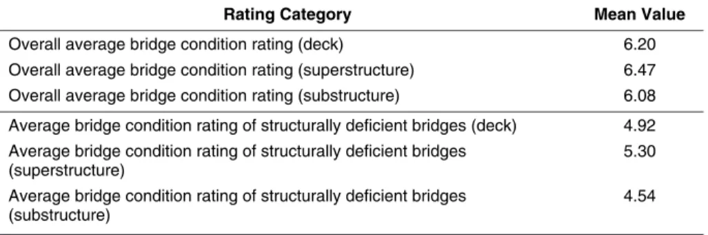
The mean values of the bridge condition rating variable for deck, superstructure, and sub-structure are shown in Table 4. These have been calculated by taking the sum of all the values and then dividing by the total number of cases (100 in this example). Generally, a condition rating

Bridge

No. Owner Location

Bridge Condition Rating _Overall

Condition Deck Superstructure Substructure

1 State Rural 8 8 8 ND*

7 Local agency Rural 6 6 6 FO*

39 State Urban 6 6 2 SD*

69 State park Rural 7 5 5 SD

92 City Urban 5 6 6 ND

*ND = not deficient; FO: functionally obsolete; SD: structurally deficient.

Table 2. Sample bridge inspection data.

Structurally Deficient (SD),

13%

Functionally Obsolete (FO),

10% Neither SD/FO,

77%

(23)

of 4 or below indicates deficiency in a structural component. For the purpose of comparison, the mean bridge condition rating of the 13 structurally deficient bridges also is provided.

Notice that while the rating scale for the bridge conditions is discrete with values ranging from 0 (failure) to 9 (excellent), the average bridge condition variable is continuous. Therefore, an average score of 6.47 would indicate overall condition of all bridges to be between 6 (satisfactory) and 7 (good). The combined bridge condition rating of deck, superstructure, and substructure is not defined; therefore calculating the mean of the three components’ average rating would make no sense. Also, the average bridge condition rating of functionally obsolete bridges is not calculated because other functional characteristics also accounted for this designation.

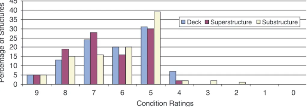
The distributions of the bridge condition ratings for deck, superstructure, and substructure are shown in Figure 2. Based on the cut-off point of 4, approximately 7% of all bridge decks, 2% of all superstructures, and 5% of all substructures are deficient.

5. Interpreting the Results: The results indicate that a majority of bridges (77%) are not

struc-turally or functionally deficient. The inspections were carried out on bridges primarily located in rural areas (88 out of 100). The bridge condition variable may also be cross-tabulated with the ownership variable to determine distribution by jurisdiction. The average condition ratings for the three bridge components for all bridges lies between 6 (satisfactory, some minor problems) and 7 (good, no problems noted).

6. Conclusion and Discussion: This example illustrates how to summarize and present

quan-titative and qualitative data on bridge conditions. It is important to understand the mea-surement scale of variables in order to interpret the results correctly. Bridge inspection data collected over time may also be analyzed to determine trends in the condition of bridges in a given area. Trend analysis is addressed in Example 15 (structures).

7. Applications in Other Areas of Transportation Research: Descriptive statistics could be

used to present data in other areas of transportation research, such as:

• Transportation Planning—to assess the distribution of travel times between origin-destination pairs in an urban area. Overall averages could also be calculated.

• Traffic Operations—to analyze the average delay per vehicle at a railroad crossing.

Rating Category Mean Value

Overall average bridge condition rating (deck) 6.20

Overall average bridge condition rating (superstructure) 6.47 Overall average bridge condition rating (substructure) 6.08 Average bridge condition rating of structurally deficient bridges (deck) 4.92 Average bridge condition rating of structurally deficient bridges

(superstructure) 5.30

Average bridge condition rating of structurally deficient bridges

(substructure) 4.54

Table 4. Bridge condition ratings.

Rural Urban Total

Structurally deficient 10 (11.4%) 3 (25.0%) 13 Functionally obsolete 6 (6.8%) 4 (33.3%) 10

Not deficient 72 (81.8%) 5 (41.7%) 77

Total 88 (100%) 12 (100%) 100

(24)

• Traffic Operations/Safety—to examine the frequency of turning violations at driveways with various turning restrictions.

• Work Zones, Environment—to assess the average energy consumption during various stages of construction.

Example 2: Public Transport; Descriptive Statistics

Area: Public transport

Method of Analysis: Descriptive statistics (organizing and presenting data to describe a system

or component)

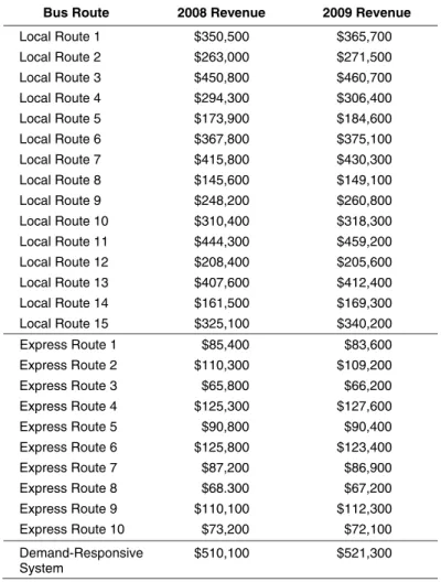
1. Research Question/Problem Statement: The manager of a transit agency would like to present

information to the board of commissioners on changes in revenue that resulted from a change in the fare. The transit system provides three basic types of service: local bus routes, express bus routes, and demand-responsive bus service. There are 15 local bus routes, 10 express routes, and 1 demand-responsive system.

0 5 10 15 20 25 30 35 40 45

9 8 7 6 5 4 3 2 1 0

Condition Ratings

Percentage of Structures

Deck Superstructure Substructure

Figure 2. Bridge condition ratings.

Question/Issue

Use data to describe some change over time. In this instance, data from 2008 and 2009 are used to describe the change in revenue on each route/part of a transit system when the fare structure was changed from variable (per mile) to fixed fares.

2. Identification and Description of Variables: Revenue data are available for each route on

the local and express bus system and the demand-responsive system as a whole for the years 2008 and 2009.

3. Data Collection: Revenue data were collected on each route for both 2008 and 2009. The annual

revenue for the demand-responsive system was also collected. These data are shown in Table 5.

4. Specification of Analysis Technique and Data Analysis: The objective of this analysis is

to present the impact of changing the fare system in a series of graphs. The presentation is intended to show the impact on each component of the transit system as well as the impact on overall system revenue.

The impact of the fare change on the overall revenue is best shown with a bar graph (Figure 3). The variation in the impact across system components can be illustrated in a similar graph (Figure 4).

(25)

Bus Route 2008 Revenue 2009 Revenue

Local Route 1 $350,500 $365,700

Local Route 2 $263,000 $271,500

Local Route 3 $450,800 $460,700

Local Route 4 $294,300 $306,400

Local Route 5 $173,900 $184,600

Local Route 6 $367,800 $375,100

Local Route 7 $415,800 $430,300

Local Route 8 $145,600 $149,100

Local Route 9 $248,200 $260,800

Local Route 10 $310,400 $318,300

Local Route 11 $444,300 $459,200

Local Route 12 $208,400 $205,600

Local Route 13 $407,600 $412,400

Local Route 14 $161,500 $169,300

Local Route 15 $325,100 $340,200

Express Route 1 $85,400 $83,600

Express Route 2 $110,300 $109,200

Express Route 3 $65,800 $66,200

Express Route 4 $125,300 $127,600

Express Route 5 $90,800 $90,400

Express Route 6 $125,800 $123,400

Express Route 7 $87,200 $86,900

Express Route 8 $68.300 $67,200

Express Route 9 $110,100 $112,300

Express Route 10 $73,200 $72,100

Demand-Responsive

System $510,100 $521,300

Table 5. Revenue by route or type of service and year.

6.02 6.17

0 1 2 3 4 5 6 7 8

2008 2009

Total System Revenue

Revenue (Million $)

(26)

Express Buses,

15.7% Express Buses,15.2%

Local Buses, 76.3% Local Buses,

75.8%

Demand Responsive,

8.5%

Demand Responsive,

8.5%

2008 2009

Figure 5. Pie charts illustrating percent of revenue from each component of a transit system.

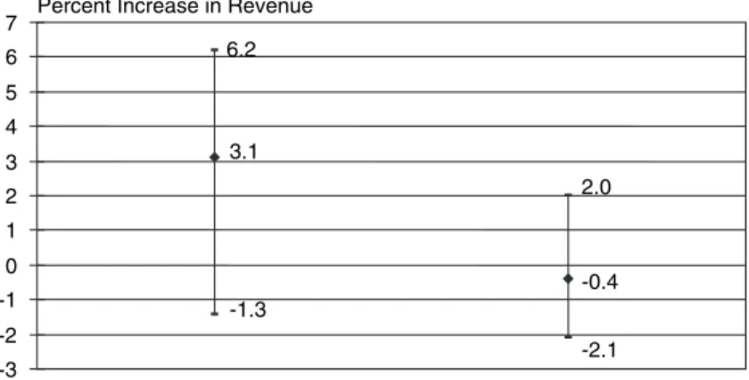
If it is important to display the variability in the impact within the various bus routes in the local bus or express bus operations, this also can be illustrated (Figure 6).

This type of diagram shows the maximum value, minimum value, and mean value of the percent increase in revenue across the 15 local bus routes and the 10 express bus routes.

5. Interpreting the results: These results indicate that changing from a variable fare based

on trip length (2008) to a fixed fare (2009) on both the local bus routes and the express bus routes had little effect on revenue. On the local bus routes, there was an average increase in revenue of 3.1%. On the express bus routes, there was an average decrease in revenue of 0.4%.

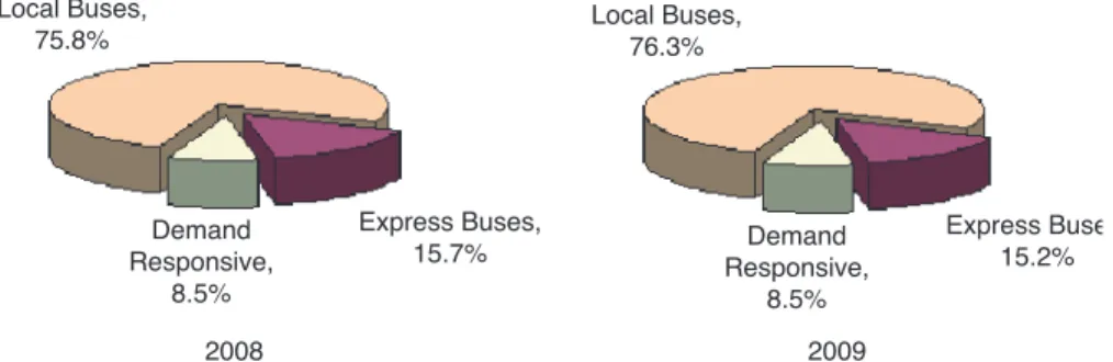
These changes altered the percentage of the total system revenue attributed to the local bus routes and the express bus routes. The local bus routes generated 76.3% of the revenue in 2009, compared to 75.8% in 2008. The percentage of revenue generated by the express bus routes dropped from 15.7% to 15.2%, and the demand-responsive system generated 8.5% in both 2008 and 2009.

6. Conclusion and Discussion: The total revenue increased from $6.02 million to $6.17 mil lion.

The cost of operating a variable fare system is greater than that of operating a fixed fare system— hence, net income probably increased even more (more revenue, lower cost for fare collection), and the decision to modify the fare system seems reasonable. Notice that the entire discussion

Figure 4. Variation in impact of fare change across system components.

0.94

0.51 0.94

0.52 4.57

4.71

0 0.5 1 1.5 2 2.5 3 3.5 4 4.5 5 5.5 6

Local Buses Express Buses Demand Responsive

Revenue (Million $)

(27)

also is based on the assumption that no other factors changed between 2008 and 2009 that might have affected total revenues. One of the implicit assumptions is that the number of riders remained relatively constant from 1 year to the next. If the ridership had changed, the statistics reported would have to be changed. Using the measure revenue/rider, for example, would help control (or normalize) for the variation in ridership.

7. Applications in Other Areas in Transportation Research: Descriptive statistics are widely

used and can convey a great deal of information to a reader. They also can be used to present data in many areas of transportation research, including:

• Transportation Planning—to display public response frequency or percentage to various alternative designs.

• Traffic Operations—to display the frequency or percentage of crashes by route type or by the type of traffic control devices present at an intersection.

• Airport Engineering—to display the arrival pattern of passengers or flights by hour or other time period.

• Public Transit—to display the average load factor on buses by time of day.

Example 3: Environment; Descriptive Statistics

Area: Environment

Method of Analysis: Descriptive statistics (organizing and presenting data to explain current

conditions)

1. Research Question/Problem Statement: The planning and programming director in

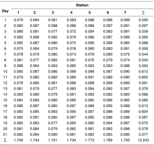
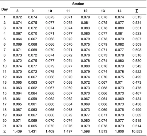
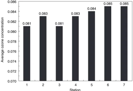
Envi-ronmental City wants to determine the current ozone concentration in the city. These data will be compared to data collected after the projects included in the Transportation Improvement Program (TIP) have been completed to determine the effects of these projects on the environ-ment. Because the terrain, the presence of hills or tall buildings, the prevailing wind direction, and the sample station location relative to high volume roads or industrial sites all affect the ozone level, multiple samples are required to determine the ozone concentration level in a city. For this example, air samples are obtained each weekday in the month of July (21 days) at 14 air-sampling stations in the city: 7 in the central city and 7 in the outlying areas of the city. The objective of the analysis is to determine the ozone concentration in the central city, the outlying areas of the city, and the city as a whole.

Figure 6. Graph showing variation in revenue increase by type of bus route.

-0.4 -1.3

-2.1 3.1

6.2

2.0

-3 -2 -1 0 1 2 3 4 5 6 7

Local Bus Routes Express Bus Routes

(28)

2. Identification and Description of Variables: The variable to be analyzed is the 8-hour

average ozone concentration in parts per million (ppm) at each of the 14 air-sampling stations. The 8-hour average concentration is the basis for the EPA standard, and July is selected because ozone levels are temperature sensitive and increase with a rise in the temperature.

3. Data Collection: Ozone concentrations in ppm are recorded for each hour of the day at each of

the 14 air-sampling stations. The highest average concentration for any 8-hour period during the day is recorded and tabulated. This results in 294 concentration observations (14 stations for 21 days). Table 6 and Table 7 show the data for the seven central city locations and the seven outlying area locations.

4. Specification of Analysis Technique and Data Analysis: Much of the data used in analyzing

transportation issues has year-to-year, month-to-month, day-to-day, and even hour-to-hour variations. For this reason, making only one observation, or even a few observations, may not accurately describe the phenomenon being observed. Thus, standard practice is to obtain several observations and report the mean value of all observations.

In this example, the phenomenon being observed is the daily ozone concentration at a series of air-sampling locations. The statistic to be estimated is the mean value of this variable over

Question/Issue

Use collected data to describe existing conditions and prepare for future analysis. In this example, air pollution levels in the central city, the outlying areas, and the overall city are to be described.

Day

Station

1 2 3 4 5 6 7 ∑

1 0.079 0.084 0.081 0.083 0.088 0.086 0.089 0.590

2 0.082 0.087 0.088 0.086 0.086 0.087 0.081 0.597

3 0.080 0.081 0.077 0.072 0.084 0.083 0.081 0.558

4 0.083 0.086 0.082 0.079 0.086 0.087 0.089 0.592

5 0.082 0.087 0.080 0.075 0.090 0.089 0.085 0.588

6 0.075 0.084 0.079 0.076 0.080 0.083 0.081 0.558

7 0.078 0.079 0.080 0.074 0.078 0.080 0.075 0.544

8 0.081 0.077 0.082 0.081 0.076 0.079 0.074 0.540

9 0.088 0.084 0.083 0.085 0.083 0.083 0.088 0.594