Solving Mathematical Problems by Parallel Processors

(1)

Solving Mathematical Problems by Parallel Processors

Dr. M Raja Sekar

Department of Computer Science & Engineering VNR VJIET, Hyderabad, Telangana,

rajasekarm9[at]gmail[dot]com

Abstract — the use of parallel processors to solve mathematical and numerical problems is growing rapidly from the past few decades. In this study, we designed a methodology that solves many mathematical and numerical problems with high computational speed. In many real time or real life applications very often we need to perform a lot of numerical computations, which may range from matrix multiplication, polynomial interpolation, solving polynomial equations, solving system of equations and so on. We consider the use of parallel processors to solve some numerical problems, namely Lagrange interpolation and polynomial root finding. The experiments were conducted on the financial dataset obtained from publicly available AWS database. We tested proposed algorithms on two different models of parallel processors and achieve the performance of O (log n).

Keyword: — Time complexity, ring, Lagrange interpolation, Durand-Kerner methods and mesh of trees.

I.INTRODUCTION

Polynomial interpolation is heavily used in geological mapping, cardiology, petroleumexploration etc. Similarly in digital signal procesing, automatic control etc. Often we require fast extraction of all the roots of a high degree polynomial equation[1,2,3 and 4]. Solution to such problems are usually based on some standard numerical methods. However, the computations involved in these techniques are usually performed through some sequential steps and hence are very slow and cannot fulfill the demand of the real time or real life applications. Therefore, the sequential algorithms of these computations are usually not encouraged in solving the problems in the above applications. Efficient parallelization of various steps in these computations is thus called for so as to reduce the total execution time for effectively using them in the above applications. Design of efficient parallel algorithms for such problems has thus become one of the research areas in the field of parallel processing. In

this study we present two parallel algorithms for the solution of two numerical problems namely polynomial interpolation and solving polynomial equation. For the polynomial interpolation, we choose Lagrange interpolation and we use Durand-Kerner and Ehrlich methods for solving polynomial equation. The algorithms are run on two different models of parallel computers, namely mesh of trees and ring [5, 6 and 7]. The resto f the paper is organized as follows. We describe the parallel algorithm in section 2. The parallel algorithm of the Durand-Kerner method is presented in section 3 followed by a conclusion in section 4.

II.LAGRANGESINTERPOLATION

The italic n-point Lagrange interpolation formula is formula is follows [13]:

In recent years, many parallel algorithms have been reported for polynomial interpolation in the literature [8, 9, 10, 11, 12, 13 and 14]. Capello, Gallopolous and Koc [15] presented a systolic algorithm that uses 2n-1 steps on n/2 processors in which each step required two substractions and one divison. In [16] another systalic algorithm has been described with O(n) time complexity. A parallel algorithm for rational interpolation has been reported in [17] with the time complexity of O(n) on n+1 processors. A parallel algorithm for Lagrange interpolation has been described in [18]. I tis shown that the algorithms runs in O(log n) time tusing n2 processors. Ben Goertzel [19] presented a parallel algorithm for the evaluation of n-point Lagrange interpolating polynomial that use n/2+ O(log n) steps

P

(

x

)

=

Õ

(

x

)

y

i

(

x

-

x

_i

)

Õ

(

x

_i

)

é

ë

ê

ù

û

ú

i=0 n-1

å

(1)

y

_i

=

f

(

x

_i

)

Õ

(

x

)

=

(

x

-

x

₀

)(

x

-

x

₁

)(

x

-

x

₂

)...(

x

-

x

_n_-₁

)

(2)

on an n processor tree with additional ring connections. The parallel algorithm described in [6] has the time complexity of O(log n3_{) on an} EREW-PRAM model. For the parallel implementation, we choose the model of computation as described below.

2.1 Mesh of Trees (Computational Model)

We use an nxn mesh of trees (MOT) [8] consisting of n2_{processors organized as follows:}

1.Processors are placed in an nxn lattice with n rows and n columns. The processors placed in the th row and the th_{column is denoted by P(}__,__). 2.In the th _{row, 1<}__{<n, the processor P(}__,__{) is}

directly connected to the processors P(, 2) and the P(, 2+1) if they exist for  =1 to n/2.That is there exist a binary tree connection in every row , 1<<n rooted at P(1, ).

3.Every processor has three logical registers, namely B(, ), A(, ) and C(, ) in the order.

III. FIRST PROPOSAL ALGORITHM

Step 1. For all =1 to n do in parallel

1.1 A(, 1)=x;

1.2 Broadcast the content of A(, 1) to A(, ) , 1<<n using binary tree connection.

1.3 C(, ) = A(, ).

2.1 A(, 1)=x-1 .

Broadcast the content of A(, 1) to A(, ), 1<<n using binary tree connection along the th _row.

2.2 B(1, ) = x-1 .

Broadcast the content of B(1, ) to B(, ), 1<<n using binary tree connection along the th _column.

2.3 A(, )= C(, )

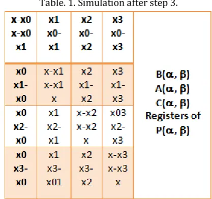
Step 3. For all  and  =1 to n do in parallel

3.1 A(, ) = A(, ) - B(, ) 3.2 B(,) = A(,)

The contents of the registers after this step as shown in table. 1.

4.1. Using the tree connection, compute the product of the contents of A(, ), 1<<n along the th _row and store it in A(, 1).

Table. 1. Simulation after step 3.

Step 5. For all =1 to do in parallel Move the contents of B(, ) to B(1, ).

Step 6. Using tree connection along the first row, compute the product of the contents of B (1,), 1<<n and store in B (1, 1).

Step 7. C (1, 1) =B (1, 1).

Step 8. For all  =1 to n do in parallel

8.1 B(,1) = A(,1)

8.2 A(, 1)=y

8.3 B(,1) = A(,1)/ B(,1)

Step 9. For all =1 to n do in parallel Using tree connection along the first column sum up the contents B(,1) and store the result in B(1, 1).

Step 10. B (1, 1) =B (1, 1) *D (1, 1)

Step 11. Stop

The final interpolated value emerges from the register B (1, 1).

(3)

an nth _{degree polynomial equation say, where, the} coefficients ai’s i=0, 1, 2… n are assumed to be real.

Many software routines are available for finding the roots of a polynomial equation. The algorithms used in these library routines determine approximations to the polynomial roots by deflation method and hence provide very little scope for parallelization. However, there exist classes of algorithms, which are more suitable for parallelization. Durand-Kerner algorithm and Ehrilich algorithms are of this kind. In the recent years there has been reported several parallel algorithms based on Durand-Kerner and Ehrilich methods and can be found in the literature [9, 10, 11 and 12]. In these algorithms main attempt has been made to parallelize the computation involved in a single iteration. The iterative schemes to find the roots due to Durand-Kerner and Ehrlich are given as follows [9].

Equation 4 represents Durand-Kerener

Equation 5 represents Ehrlich Kerner

Where

The Durand-Kerner and Ehrlich methods are locally convergent with quadratic and cubic rate of convergence respectively [9]. We now present the parallel algorithm for a single iteration of the Durand-Kerner method. Because of the similarity of the computation, the parallel algorithm for

Ehrlich method can similarly be developed. We use the following computational model.

4.1 Ring Computation Model

1.n processors are arranged to form a ring. The

processors Pi is directly connected to the processor Pi mod n +1, for i=1, 2... n by means of a bi-directional links.

2.Each processor Pi has four local registers namely A (i), B (i), C (i) and D (i). The registers A (i)’s and B (i)’s are used for the data communication in the clockwise and anti-clockwise respectively.

4.2 Second Proposed Algorithm Step 1. For all =1 to n do in parallel

A (i) =xi, B (i) =xi

C (i) =xi, D (i) =1

Step 2.for k=1 to n/2-1 do

For all =1 to n do in parallel

A ( MOD n +1) =A ()

B () =A ( MOD n +1)

D () =D ()*[C ()-A ()]*[C ()-()]

A ( MOD n +1) =A ()

If (n is odd) then

B () =A ( MOD n +1)

D () =D ()*[C ()-A ()]*[C ()-()]

Else

D () =D ()*[C () - A ()]

A () =Pn(x)

D () =C ()--A ()/D ()

Step 6. Stop

P

_n

(

x

)

=

a

₀

x

n

+

a

₁

x

n-1

+

a

₂

x

n-2

+

...

+

a

_n_-₁

x

+

a

_n

=

0(3)

x_i(k+1)₌_x i

(k)_- Pn(xi (k)

)

(xi (k)-_x

j (k)

)

j=1,j¹i N

Õ

,i=1,2,....,n(4)

x

_i(k+1)

=

_x

i

(k)

_-

a

i (k)

1 -

a

_i(k)

b

_i(k)

,

i

=

1, 2,....,

n

(5)

b

i

(k)

₌

1 x

_i(k)

_-

_x

j

(k) j=1,j¹i

n

å

(6)

a

i

(k)

₌

1 y

i (l)

_-

_y

j (m) j=1,j¹i

m

(4)

It is easy to note that only step 2 requires O(n) time and the resto f steps require constant time. Hence the overall time complexity of the above algorithm is O(n) time.

V. RESULT AND CONCLUSION

The algorithms for solving the problem have been implemented in java with open MP directives. The experiments carried out on dual processor Quad-Core Xeon (3.2 GHz, 12 MB L2 cache, 32 GB RAM running under Linux) workstation using Intel Java compiler shows that new algorithm achieves much better performance than simple scalar algorithm. Table2 shows exemplary results of the performance of the algorithm for various problem sizes and block sizes. The performance of the new parallel non-square algorithm is much better. The performance is better for the bigger problem size (n=3097157) and the algorithm achieve reasonable speedup. We have shown that the performance of proposed algorithms for solving financial data is highly improved by using parallel processing. As the calculation time complexity of large problems with various constraints and variables is significant, calculation of set of problems are performed in parallel.

Table2 : Exemplary results of the performance of proposed algorithm on dataset1

The proposed system gives the solutions in very effective and accurate manner. These results are useful in solving structural engineering case studies with lots of uncertain constraints. These results describe in depth analysis of parallel processing which makes use the knowledge of computer science, mathematics and probability. The accuracy of the results is achieved by proper analysis, optimization and modeling of large set of financial problems with several constraints. The results shown in Table2, Table3 and Table4 describe the accuracy of different data sets of financial data obtained from AWS database.

Table3 : Exemplary results of the performance of proposed algorithm on dataset2.

Table4 : Exemplary results of the performance of proposed algorithm on dataset3.

(5)

been shown to run in O(log n) tim eon a mesh of trees model of parallel computers. For solving polynomial equation of degree n, we have shown the parallelization of Durand-Kerener method on ring of n processors in O(log n) time.

REFERENCE

[1]. Dr. M Raja Sekar et al., “Tongue Image Analysis

For Hepatitis Detection Using GA-SVM," Indian Journal of computer science and Engineering, Vol 8 No 4 , pp. , August 2017.

[2]. Dr. M Raja Sekar et al, " Mammogram Images

Detection Using Support Vector Machines," International Journal of Advanced Research in Computer Science “,Volume 8, No. 7 pp. 329-334, July – August 2017.

[3]. Dr. M Raja Sekar et al., " Areas categorization by

operating support Vector machines”, ARPN Journal of Engineering and Applied Sciences”, Vol. 12, No.15 , pp.4639-4647 , Aug 2017.

[4]. Dr. M Raja Sekar, “Diseases Identification by GA

-SVMs”, International Journal of Innovative Research in Science, Engineering and Technology, Vol 6, Issue 8, pp. 15696-15704, August 2017.

[5]. Dr. M Raja Sekar., “Classification of Synthetic

Aperture Radar Images using Fuzzy SVMs”, International Journal for Research in Applied Science & Engineering Technology (IJRASET) , Volume 5 Issue 8, pp. 289-296 , Vol 45, August 2017.

[6]. Dr. M Raja Sekar, “Breast Cancer Detection using

Fuzzy SVMs”, International Journal for Research in Applied Science & Engineering Technology (IJRASET)”, Volume 5 Issue 8, pp. 525-533, Aug ,2017.

[7]. Dr. M Raja Sekar, “Software Metrics in Fuzzy

Environment “ , International Journal of Computer & Mathematical Sciences(IJCMS) , Volume 6, Issue 9, September 2017.

[8]. Dr. M Raja Sekar, “Interactive Fuzzy Mathematical

Modeling in Design of Multi-Objective Cellular Manufacturing Systems”, International Journal of Engineering Technology and Computer Research (IJETCR), Volume 5, Issue 5, PP 74-79, September-October: 2017.

[9]. Dr. M Raja Sekar, “Optimization of the Mixed

Model Processor Scheduling”, International Journal of Engineering Technology and Computer Research (IJETCR), Volume 5, Issue 5, pp 74-79, September-October: 2017.

[10]. Cosnard, M., and P. Fraigniaud, “Finding the roots

of the polynomial on an MIMD multi computer “, parallel computing , Vol. 15, pp. 75-85, 2015.

[11]. Freeman, T.L.”Calculating polynomial zeros on

local member parallel computer “, Prentice Hall, 2016.

[12]. M. Raja Sekar, “Automatic Vehicle Identification”

Journal of Advanced Research in Computer Engineering, pp 0974-4320, 2015.

[13]. M. Raja Sekar “FER from Image sequence using

SVMs “, Journal of Data Engineering and computer science, pp 80- 89, 2016.

[14]. M. Raja Sekar, “ImageAuthentication using SVMs”,

Journal of Advanced Research in computer Engineering, p367-p374, 2015.

[15]. M. Raja Sekar, “Classification of images using

SVMs”, International Journal of Mathematics, Computer Sciences and Information Technology, p25-29, 2014.

[16]. M. Colombo, J. Gondzio and A. Grothey, “A Warm

-Start Approach for Large-Scale Stochastic Linear Programs, Tech. Rep. MS-06-004, School of Math’s, University of Edinburgh, 2015.

[17]. J. Gondzio and A. Grothey, Parallel interior point

solver for structured quadratic programs: application to financial planning problems, Annals of OR 152, vol 1, pp 319-339, 2016.

[18]. J. Gondzio and A. Grothey, Solving nonlinear