Curvature and Histogram of oriented Gradients based 3D Face Recognition using Linear Discriminant Analysis

(1)

Journal of Multimedia and Information System Vol. 2, No 1, March 2015(pp. 171-178): ISSN 2383-7632(Online) http://dx.doi.org/10.9717/jmis.2015.2.1.171

171

I. INTRODUCTION

The ability to recognize a person is a task that human risibly performs but one that computers to date have been unable to perform robustly. For the automatic user identification or surveillance, various researches using human face information are performed using biometric information (fingerprint, face, iris, voice, vein, etc.) [1]. In a biometric identification system, the face recognition with a non-touch style is a very challenging research area, next to the fingerprint. Many different human face recognition algorithms have been developed and motivated by the face recognition is non-touch style, for the last 30 years [1]. There are several problems that are easily influenced by lighting illuminance and encountered difficulties when the face is angled away from the camera, especially in two dimensional face recognition systems. To solve these problems, a 3D face recognition system using stereo matching, laser scanner and etc. has been developed [2-3].

Broadly speaking, two approaches have emerged to recognize the face. One type employs the facial feature

based approach and the other is the area based approach [4-5]. Recently, as the 3D system is being cheaper, smaller, and faster than it used to be, the research on the 3D face image is performed more actively [2-3]. Many researchers have used differential geometry tools for computing the curvatures in 3D face [6]. Hiromi et al. [7] treated the problem of 3D shape recognition with rigid free-form surfaces. Each face in the input images and the model database are represented as an Extended Gaussian Image (EGI), constructed by mapping principal curvatures and their directions. Gordon [8] presented the study of face recognition based on depth and curvature features. To find face specific descriptors, he used the curvatures of the face. Comparison of the two faces was made based on the relationship between the spacing of the features. Lee and Milios [9] extracted the convex regions of the face by segmenting the range of the images based on the sign of the mean and Gaussian curvature at each point. For each of these convex regions, the Extended Gaussian Image (EGI) was extracted and then used to match the facial features of the two face images. One of the most successful techniques of the face recognition as statistical method is principal component analysis (PCA),

Curvature and Histogram of oriented Gradients based 3D Face

Recognition using Linear Discriminant Analysis

Author: Yeunghak Lee

1,*

Abstract

This article describes 3 dimensional (3D) face recognition system using histogram of oriented gradients (HOG) based on face curvature. The surface curvatures in the face contain the most important personal feature information. In this paper, 3D face images are recognized by the face components: cheek, eyes, mouth, and nose. For the proposed approach, the first step uses the face curvatures which present the facial features for 3D face images, after normalization using the singular value decomposition (SVD). Fisherface method is then applied to each component curvature face. The reason for adapting the Fisherface method maintains the surface attribute for the face curvature, even though it can generate reduced image dimension. And histogram of oriented gradients (HOG) descriptor is one of the state-of-art methods which have been shown to significantly outperform the existing feature set for several objects detection and recognition. In the last step, the linear discriminant analysis is explained for each component. The experimental results showed that the proposed approach leads to higher detection accuracy rate than other methods.

Key Words: Curvature, Histogram of oriented gradients, LDA, Face recognition

Manuscript received March 31, 2015; Revised April 20, 2015; Accepted May 10, 2015. (ID No. JMIS-2015-0010)

Corresponding Author(*): Yeunghak, Lee, Kyungwoon Univ. 55 Indoek-ri, Sandong-myeon, Gumi, Korea, +82-54-479-1215, [email protected].

1

(2)

Curvature and Histogram of oriented Gradients based 3D Face Recognition using Linear Discriminant Analysis

172

specifically eigenfaces [10-11]. However, it is not ideal for classification purpose as it retains unwanted variations occurring due to diversified face shape and face poses. To overcome this problem, proposed method was an enhancement known as the Fisherface method, or Fisher’s linear discriminant (FLD), linear discriminant analysis (LDA) [12]. Especially, Zhao et al. [22] suggested multiple feature domains based on the face recognition using the FLD through the dividing (4 types) of an original image.

The single characteristics, widely used to detect pedestrians and objects, are incorporated edge [13], appearance [14], local binary pattern (LBP) [15], histogram of oriented gradients (HOG) [16], Haar-like [17] and wavelet coefficient [18]. HOG characteristics or improved HOG characteristics are widely utilized in the methods for the recognizing pedestrians by using the automobile vision. Zhu et al. [19] applied the HOG characteristics based on variable block size to improve detection speed. Further, Watanabe et al. [20] utilized co-occurrence HOG characteristics, and Wang et al. [21] utilized HOG-LBP human detection to improve detection accuracy.

In this paper, a novel face recognition method is introduced using the face curvatures and histogram of gradients oriented algorithm presented well personal characteristics and reduced the feature dimension. Moreover, the normalized facial pose images using SVD are considered to improve the recognition rate, as the preprocessing.

This paper is organized as follow. In section II, this paper explains the face pose normalization to improve the recognition rate. Section III describes the face surface curvature and HOG including personal feature information. To classify the person, linear discriminant analysis is introduced in section IV. The results of their evaluation and a detailed performance analysis are presented in section V. Section VI concludes this paper.

II. Face Pose Normalization [22]

The nose is protruded shape and located in the middle of the face. So it can be used as the reference point, firstly we tried to find the nose tip using the iterative selection method, after extraction of the face from the 3D face image [23]. Usually, face recognition systems suffer from drastic losses in performance when the face is not correctly oriented. The normalization process proposed here is a sequential procedure that aims at putting the face shapes in a standard spatial position. The processing sequence is panning, rotation and tilting.

2.1 Find Nose Tip

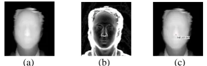
In preprocessing, a given 3D image is divided into face and background areas. Useless areas around the head and clothing parts contain too much erroneous data to process. Firstly, the nose tip is found by the iteration selection method(ISM) after using Sobel processing, as shown in Figure 1 (b).

∑∑

−

= −

=

>

= 1

0 1

0

0 , 1 M

i

img N

j

img B

P K

Avg (1)

⎩ ⎨

⎧ > =

Otherwise Avg P

P

P_img img img , 0

,

where M and N represent the size of the image. And P stands for the depth image and B is the binary image. In the result area, the new threshold value is calculated by using an average, and the new area is extracted by using P. By the repeated processes (1), the nose tip point can be found as the highest value on the range face. The results are shown in Figure 1 (c).

(a) (b) (c) Fig. 1. Preprocessing to find the nose tip using ISM (a) Original image, (b) Sobel processed image (c) The result of nose tip finding

2.2 Face Normalization

In feature recognition of 3D faces, one has to take into consideration the obtained frontal posture. Face recognition systems suffer from drastic losses in performance when the face is not correctly oriented [24]. The normalization process proposed here is a sequential procedure that aims at putting the face shapes in a standard spatial position. Obtained face poses consist of front, right rotation, left rotation, right panning, left panning, up tilt, and down tilt.

If the pose transform matrix is

A

_P

)

,

(

P

=

R

L

R

P

L

P

R

T

U

T

D ,

A

P can be calculated with

equation (2).

P P

F

A

→

Transform Matrix

A

_P: (2)

P P PF

A

C

=

+

=

F P

P

C

(3)

173

where C_PF is transformed front pose for each pose, C_P

means left rotation (RL) , right rotation (RR) , left

panning (PL), right panning (PR), up tilt (TU), and

down tilt (T_D), which has PCA coefficient matrix for all

the training sets. C+ is the pseudo inverse matrix using Singular Value Decomposition (SVD) for the matrix . The reason why we have to use is that it is difficult to get the reverse matrix from the matrix which has no square matrix. The equation (3) explains the brief algorithm for the pose transform.

1.

H

= input image (3)

2.

e

= projection Eigenface space(

H

) 3.

P

= pose estimation (

e

)

4.

e

′

= pose transform (

e

,

P

)

A

P

e

5.

H

~

= reconstruction using Eigenvector and mean face (

e

′

)

III. Surface Curvature and HOG

3.1 Surface Curvature

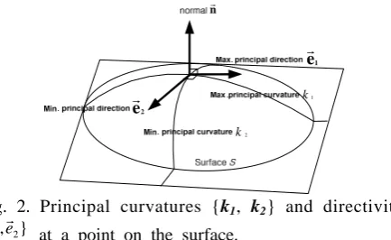
For each data point on the facial surface, the principal, Gaussian and mean curvatures are calculated and the signs of those (positive, negative and zero) are used to determine the surface type at every point. The z(x, y) image represents a surface where the individual Z-values are surface depth information. The curvatures and related variables are computed for the pixel at location(0,0). Each pixel has an intensity value, a gray ton value or a depth value z(x,y). These intensity values define a surface in a three dimensional space as shown in Figure 2.

e2

r

e1

r

k2

k1

nr

Fig. 2. Principal curvatures {k1, k2} and directivity }

,

{er₁ er₂ _{at a point on the surface.}

Here, x and y are the two spatial coordinates. We now closely follow the formalism introduced by Peet and Sahota [25], and specify any point on the surface by its position vector:

k y x z yj xi y x

R( , )= + + ( , ) (4)

The first fundamental form of the surface is the expression for the element of arc length of curves on the surface which pass through the point under consideration. It is given by:

2 2

2

2Fdxdy Gdy

Edx dR dR ds

I = = ⋅ = + + (5)

where

2

1 ⎟

⎠ ⎞ ⎜ ⎝ ⎛ ∂ ∂ + =

x z

E ,

y z x z F

∂ ∂ ∂ ∂

= ,

2

1 _⎟⎟

⎠ ⎞ ⎜⎜ ⎝ ⎛ ∂ ∂ + =

y z

G (6)

The second fundamental form arises from the curvature of these curves at the point of interest and in the given direction:

2 2

2fdxdy gdy edx

II= + + (7)

where

Δ ∂ ∂ = 2₂

x z

e , Δ

∂ ∂

∂ =

y x

z f

2

, Δ

∂ ∂ = 2₂

y z

g (8)

and

2 / 1 2

)

( − −

=

Δ EG F (9)

Casting the above expression into matrix form with;

⎟⎟ ⎠ ⎞ ⎜⎜ ⎝ ⎛ =

dy dx

V , _⎟⎟

⎠ ⎞ ⎜⎜ ⎝ ⎛ =

G F

F E

A , _⎟⎟

⎠ ⎞ ⎜⎜ ⎝ ⎛ =

g f

f e

B (10)

the two fundamental forms become:

AV V I= t

BV V I = t

(11)

Then the curvature of the surface in the direction defined by V is given by:

AV V

BV V

k _t

t

= (12)

Extreme values of k are given by the solution to the eigenvalue problem:

0 )

(B−kAV = (13)

or

0

= − −

− −

kG g kF f

kF f kE e

(14)

which gives the following expressions for k1 and k2, the

(4)

174

{

2

1 gE 2Ff Ge [(gE Ge 2Ff)

k = − + − + −

}

/2( ) )]

)( (

4 2 2 1/2 2

F EG F

EG f

eg− − −

− (15)

(12)

{

2

2 gE 2Ff Ge [(gE Ge 2Ff)

k = − + + + −

}

/2( ) )]

)( (

4 2 2 1/2 2

F EG F

EG f

eg− − −

− (16)

(13)

Here we have ignored the directional information related to k1 and k2, and chosen k2 to be the larger of the

two. For the present work, however, this has not been done. The two quantities, k1 and k2, are invariant under rigid

motions of the surface. This is a desirable property for us since the cell nuclei have no predefined orientation on the slide (the x – y plane).

The Gaussian curvature K and the mean curvature M are defined by

2 1k

k

K= , M =

( )

k1k2 /2 (17) (14)

which gives k1 and k2, the minimum and maximum

curvatures, respectively. It turns out that the principal curvatures, k1 and k2, and Gaussian are best suited to the

detailed characterization for the facial surface, as illustrated in Fig. 1. For the simple facet model of the second order polynomial of the form, i.e. a 3 by 3 window implementation in our range images, the local region around the surface is approximated by a quadric

xy a y a x a y a y a x a a y x

z 11

2 02 2 20 01 01 10 00

) ,

( = + + + + + + (18) (15)

and the practical calculation of principal and Gaussian curvatures is extremely simple.

3.2 Histogram of Oriented Gradients

HOG [23] converts the distribution directions of brightness for a local region into a histogram to express them in feature vectors, which is utilized to express the shape characteristics of an object. And it is influenced a little from an effect of illumination by converting the distribution of near pixels for a local region into a histogram, and has a strong feature for a geometric change of local regions. The following is a detailed explanation on how HOG description is calculated.

3.2.1 Gradient Computation

Value of gradient at every image pixel is calculated by derivatives fx and fy in x and y direction by convolving the

filter mask [-1 0 1] and [-1 0 1]T. Refer equation (19) and (20).

]

1

0

1 [

−

⊗

=

I

f

x (19)

T y

I

f

=

⊗

[

−

1

0

1 ]

(20)

where I is an example gray scale image and ⊗is the convolution operation. The gradient magnitudes m(x,y)

and orientation direction θ(x,y) for each pixel are

calculated by

( )

2

( )

2

, ,

) ,

(x y f x y f x y

m = _x + _y (21)

( )

⎟⎟

⎠ ⎞ ⎜

⎜ ⎝ ⎛ =

y x f

y x f y

x

x y

, , arctan ) , (

θ (22)

3.2.2 Orientation Binning

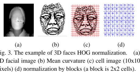
This stage defines production of an encoding that is sensitive to local image content. The image windows are divided into 8x8 rectangular small spatial regions call cells, as shown in figure 1 (c). Similar to [20], we used unsigned gradients in conjunction with nine bins for every cell (a bin corresponds to 20o). The 8x8 cell magnitude pixels are accumulated in one of the nine bins according to their orientation direction. Figure 1 (c) depicts a graphical representation on how the gradient angle range is binned in its respective cell

(a) (b) (c) (d) Fig. 3. The example of 3D faces HOG normalization. (a) 3D facial image (b) Mean curvature (c) cell image (10x10 pixels) (d) normalization by blocks (a block is 2x2 cells).

3.2.3 Block Normalization

Directional histograms for brightness prepared in each of the cells were normalized as a block of 3x3 cells. This is performed by grouping cells in larger spatial regions called blocks. Characteristic quantities (9 dimensions) of row i, column j, Cell (i, j) are expressed as Fi,j=[F1, F1,

··· ,F9]. The characteristic quantities of k’th block (81

dimensions) may be expressed as:

[

,

+1

,

+2

,

+1

,

+2

=

_ij _i _j _i _j _ij _ij

k

F

B

]

2 2 2 1 1 2 1

1 +

,

+ +

,

+ +

,

+ +

+ j i j i j i j

i

F

(23)

(5)

J h 1 m i c F w n s f f P c i m { t t t m m r

X

m t w m T

Journal of Mult http://dx.doi.org/1 175 method. The mportant fea characteristic v

=

Π

k

B

For example, width of an in number of the size of block feature vectors

IV. L

LDA[12] sea face images of PCA), and at t class are close n the scene t more useful f } , , ,

{x₁ x₂ _K x_N

the c classes{

transformation the between-c maximized. M matrix and the

∑

= = c i i B N

S

1

∑ ∑

= ∈ = c i x W k

S

1

respectively, w

i

X

and

N

i

X

. If

S

_Wis

matrix

W

_opt

the between-c within-class s matrix is repre

m arg

opt

W

=

The set of th

timedia and Info 10.9717/jmis.201

overlapping p atures of eac

vectors are giv

(

2 2

=

+

ε

k k

B

the dimensio nput image are e histogram is is 3, then th s with 6804 di

Linear Disc

arches for the f different are the same time e from each ot that it can re for classificat } , assuming

, , ,

{X1 X2 K X

n matrix W class scatter a Mathematicall e within-class

−

− i

i i(μ μ)(μ

∑

∈ − X k i k i x x )( ( μ

where

μ

_i de

i

N

denotes the

s nonsingular,

maximizing t

class scatter m scatter matrix esented by max W T B T

W _W _S _W

W S W

he solution {

formation System 5.2.1.171

process is do ch cell. And

ven by

)

1 =

on numbers fo e 128x64 pixe 9, the size of he calculated imension is ob

criminant A

e projection a e far from each e where the im ther. It is clas epresent data tion. Given a

each image b

} c

X , and LDA

in such a way and the withi ly, the betw scatter matrix − T ) μ − T i

k μ)

enotes the me

e number of im

LDA will fin

the ratio of th

matrix to the d . That is, the

[w₁ w₂

= , , 2 , 1 m i

wi = K

m Vol. 2, No 1,

one to ensure d the normal

(

for the height els, the dimen f cell is 8, and

number of H btained.

Analysis

axes on which h other (simil mages of the s ss specific me in form whic

set of N im belongs to on

A selects a li

y that the rati in-class scatte ween-class sc

x are defined a

an image of c

mages in the c

nd an orthono

he determinan

determinant of e LDA projec

]

m

w

L (

}

m is that of

March 2015(pp e the lized (24) and nsion d the HOG h the ar to same ethod ch is mages ne of inear io of er is catter as (25) class class rmal nt of f the ction (26) f the gen to th S

In o

the feat y To m the train d In cult com stra 7 po and and nos valu arou reco first Figu pos surf feat curv face the (C), com show (a Fig. seco Pann

p. 171-178): IS

neralized eige

he m largest

w S w

S_B _i =λ_i _W _i

order to overc

vector dimen ture vector is r

k x w y k T opt

k = , =

make classific Euclidean di ning set x th

y x x

d( , ′)= −

V.

this study, w ture to obtai mposed of 592 ategies: used tr oses (training d up tilt, and te d down tilt) pe e tip point is ues (for which und the nose ognition expe tly need to c ure 4. After fi e normalizati face curvature tures was obt vature distribu e components

areas, as sho , nose area mponent, LDA

wed in Table

a) (b) . 4. The examp ond front, (c)

ning, (f) Left Pa

SSN 2383-7632(

nvectors of

t eigenvalues

m i

i, =1,2,K,

come the sing

nsion before represented by N , , 2 , 1 K =

cation of new istance betwe hat is

y′

Experimen

we used a 3D in a 3D fac 2 images is us raining and te g: first front, r est: second fro er person. Wit

s found by u h the fiducial p

e area are th eriments for t create two se inding the nos ion using the e which is w tained. For th

utions are sh , four face are wn in Figure (N), and mo A and Norm

1.

(c) (d)

ple of face ima Right Rotation anning, (g) Up

(Online)

B S and

W S , 2 , 1 {λii= K

gularity of

W

S

applying LD y the vector pr

w face imagex een a given

ntal Result

laser scanner ce image [2] sed to compar est set consist

right rotation, ont left rotatio th these 3D fa using contour point is the no hen extracted the extracted ets of images

se tip, we pro e SVD. And well presented he minimum hown in Figur ea were divide 6: eye area ( outh area (M m2 recognitio

(e) (f)

ges; (a) The fir n, (d) Left rot tilt, (h) Down t

correspondin

} ,m

K , i.e.,

(27

, PCA reduce

DA. Each LDA rojections

(28

x′, we calculat image x′ an (29)

ts

made by a 4D ]. A databas re the differen of 296 image right panning on, left pannin

ace images, th line threshol ose tip). Image d. To perform

face area, w s, as shown i cessed the fac then, the fac d for persona

and maximum re 5. To mak ed according t (E), cheek are M). From eac on results ar

(g) (h)

(6)

176

(a) (b)

Fig. 5. Distribution of minimum curvature and maximum curvaturefor around the nose region; (a) 3 dimensional graph for minimum curvature, (b) 3 dimensional graph for maximum curvature

Fig. 6. Displayed each component area.

Generate the membership grade based on the LDA distance (d_i) information between the test image and the

training set produced in the previous section. Using this distance, we follow the method introduced in [26].

) / ( 1

1

i ij ij

d d n

+

= ,

∑

∈

=

k ij C n

k ij

ik n N

y

m( ) ( )/ (30)

where i=1,2,3,4, j=1,2,. . . , 296, i is the number of classifier and j is the index of the training set. And N_k is

the number of samples in kth classC_k.

The data sets have been extracted with the aid of LDA. The cheek part among the face components represented the highest recognition rate, 92.2% for norm2 and LDA. It shows that cheek area has outstanding curvature features, because of including the nose tip area and both sides of cheek. And also it means that it has very different shapes or surface feature for each person. In average analysis, the recognition of adapted curvature and HOG method showed 90.6% - k2, increased more than norm2 methods.

Additionally, in the curvature feature, k2 showed higher

recognition rate than k1.

VI. CONCLUSION

We have introduced, in this paper, a new practical implementation of a person verification system using curvature-HOG based on the component face images. The underlying motivations of our approach originate from the observation that the surface curvature of the face has

different shape based on the face components. And Ordinary HOG has two kinds of spatial region: small (cells) and large (blocks). And it is based on overlapping and dens encoding of image regions. To classify the faces, LDA and norm2 were used. It has been experimentally demonstrated that the aggregation of classifiers operating on four component face image sets generated by area based led to better classification results than norm2 method. Furthermore, we also confirmed that the curvature k2 has higher recognition rate than the k1.

From the experimental results, we proved that the process of the face recognition may use lower dimension, less parameters, and less calculation than earlier suggestion. We consider that there are many future experiments that could be done to extend this study.

Table 1. The comparision of the recognition rate (%) Method C E M N Avg.

k1 _{Norm2 92.2} _90.5_83.9_83.9 _88.5

LDA 90.8 89.9 90.2 88.7 89.9

k2 _{Norm2 89.2} _89.9_83.5_84.1 _86.7

LDA 90.8 90.8 90.2 90.5 90.6

REFERENCES

[1] L. C. Jain, U. Halici, I. Hayashi, and S. B. Lee, “Intelligent biometric techniques in fingerprint and face recognition,” CRC Press, 1999.

[2] 4D Culture, http://www.4dculture.com [3] Cyberware, http://www.cyberware.com

[4] R. Chellapa, C. L. Wilson, and S. Sirohey, “Human and Machine Recognition of Faces: A Survey,” Proceeding of the IEEE, vol. 83, no. 5, pp.705-741, May, 1995

[5] P. W. Hallinan, G. G. Gordon, A. L. Yuille, P. Giblin, and D. Mumford, “Two and three dimensional pattern of the face,” A K Peters Ltd., 1999.

[6] C. S. Chua, F. Han, and Y. K. Ho, “3D Human Face Recognition Using Point Signature,” Proc. of the 4th ICAFGR, pp.233-238, March, 2000.

[7] H. T. Tanaka, M. Ikeda, and H. Chiaki, “Curvature-based face surface recognition using spherial correlation,” Proc. of the 3rd IEEE Int. Conf. on Automatic Face and Gesture Recognition, pp. 372-377, April, 1998.

(7)

177

[9] J. C. Lee and E. Milios, “Matching range image of human faces,” Proc. of the 3rd Int. Conf. on Computer Vision, pp. 722-726, December, 1990,.

[10] M. Turk and A. Pentland, “Eigenfaces for Recognition,” Journal of Cognitive Neuroscience, vol. 3, no. 1, pp. 71-86, winter, 1991.

[11] C. Hesher, A. Srivastava, and G. Erlebacher, “Principal Component Analysis of Range Images for Facial Recognition,” Proc. of CISST, 2002.

[12] W. Zhang, S. Shan, W. Gao, Y. Chang, and B. Cao, “Component-based Cascade Linear Discriminant Analysis for Face Recognition,” Lecture Notes in Computer Science, vol. 3338, pp. 288-295, 2005. [13] D. M. Gavrila and S. Munder, “Multi-cue pedestrian

detection and tracking from a moving vehicle,” International Journal of Computer Vision, vol. 73, no. 1, pp.41-59, June, 2007.

[14] P. Sabzmeydani and G. Mori, “Detecting Pedestrians by learning shapelet features,” Proceeding of Computer Vision and Pattern Recognition, pp. 1-8, June, 2007.

[15] T. Ahonen, A. Hadid and M. Pietikainen, “Face description with local binary patters: Application to face recognition,” IEEE Transaction Pattern Analysis and machine Intelligent. vol. 28, no. 12, pp.2037-2041, October, 2006.

[16] N. Dalal and B. Triggs, “Histogram of Oriented Gradients for Human Detection,” IEEE Computer Vision Pattern Recognition, pp.886-893, June, 2005. [17] S. Pavani, D. Delgado and A. F. Frangi, “Haar-like

features with optimally weighted rectangles for rapid object detection,” Pattern Recognition, vol. 43, no. 1, January, 2010.

[18] C. Papageorgiou and T. Poggio, “A trainable system for object detection,” International Journal of Computer Vision, vol. 38, no. 1, June, 2000.

[19] Q. Zhu, M. C. Yeh, K. T. Cheng and S. Avidan, “Fast human detection using a cascade of histograms of oriented gradients,” IEEE Conference on Computer Vision and Pattern Recognition, pp. 17-22, June 2006. [20] T. Watanabe, S. Ito and K. Yokoi, “Co-occurrence

Histogram of Oriented Gradients for Detection Advances in Image and Video Technology,” Lecture Notes in Computer Science, vol. 5414, pp. 37-47, 2009. [21] X. Y. Wang, T. X. Han and S. Yan, An “HOG-LBP

human detector with partial occlusion handling,” International Conference on Computer Vision, pp. 32-39, Sept. – Oct., 2009.

[22] Y. H. Lee and D. Marshall, “Curvature based 3D component facial image recognition using fuzzy integral,” Applied Mathematics and Computation, vol. 205, pp. 815-823, 2008.

[23] Y. H. Lee, T. S. Kim, S. H. Lee, and J. C. Shim,

“New approach to two wheelers detection using Cell Comparison,” Journal of Multimedia and Information System, vol. 1, no. 1, pp. 45-53, December, 2014. [24] Peet, F. G., Sahota, T. S.: “Surface Curvature as a

Measure of Image Texture,” IEEE Trans. PAMI, vol. 7, no. 6, pp. 734-738, January, 2009.

[25]. G. Banon, “Distinction between several subsets of fuzzy measures,” Fuzzy Sets and Systems, vol. 5, no. 4, pp. 291-305, May, 1981.

[26] K. C. Kwak and W. Pedrycz, “Face Recognition using fuzzy integral and wavelet decomposition methos,” IEEE Transaction on System, Man, and Cybernetics, vol.34, no. 4, pp.1666-1675, April, 2004.

Author

(8)

178