Boundary Value Problems
Volume 2009, Article ID 905769,28pages doi:10.1155/2009/905769
Research Article
Limit Properties of Solutions of Singular
Second-Order Differential Equations
Irena Rach ˚unkov ´a,
1Svatoslav Stan ˇek,
1Ewa Weinm ¨uller,
2and Michael Zenz
21Department of Mathematical Analysis, Faculty of Science, Palack´y University,
Tomkova 40, 779 00 Olomouc, Czech Republic
2Institute for Analysis and Scientific Computing, Vienna University of Technology,
Wiedner Hauptstrasse 8-10, 1040 Wien, Austria
Correspondence should be addressed to Irena Rach ˚unkov´a,[email protected]
Received 23 April 2009; Accepted 28 May 2009
Recommended by Donal O’Regan
We discuss the properties of the differential equationut a/tut ft, ut, ut, a.e. on
0, T, wherea ∈R\{0}, andf satisfies theLp-Carath´eodory conditions on0, T×R2for some
p > 1. A full description of the asymptotic behavior fort → 0of functionsusatisfying the
equation a.e. on0, T is given. We also describe the structure of boundary conditions which are necessary and sufficient foruto be at least inC10, T. As an application of the theory, new
existence and/or uniqueness results for solutions of periodic boundary value problems are shown.
Copyrightq2009 Irena Rach ˚unkov´a et al. This is an open access article distributed under the Creative Commons Attribution License, which permits unrestricted use, distribution, and reproduction in any medium, provided the original work is properly cited.
1. Motivation
In this paper, we study the analytical properties of the differential equation
ut a tu
t ft, ut, ut, a.e.on0, T, 1.1
discontinuous inputs. Typically, such problems are modelled by differential equations where fhas jump discontinuities at a discrete set of points in0, T, compare1.
This study serves as a first step toward analysis of more involved nonlinearities, where typically,fhas singular points also inuandu. Many applications, compare2–12, showing these structural difficulties are our main motivation to develop a framework on existence and uniqueness of solutions, their smoothness properties, and the structure of boundary conditions necessary for uto have at least continuous first derivative on0, T. Moreover, using new techniques presented in this paper, we would like to extend results from13,14
based on ideas presented in15where problems of the above form but withappropriately smooth data functionfhave been discussed.
Here, we aim at the generalization of the existence and uniqueness assertions derived in those papers for the case of smoothf. We are especially interested in studying the limit properties ofufort → 0 and the structure of boundary conditions which are necessary and sufficient foruto be at least inC10, T.
To clarify the aims of this paper and to show that it is necessary to develop a new technique to treat the nonstandard equation given above, let us consider a model problem which we designed using the structure of the boundary value problem describing a membrane arising in the theory of shallow membrane caps and studied in10; see also6,9,
t3utt3
1 8u2t−
a0
utb0t
2γ−4
0, 0< t <1, 1.2
subject to boundary conditions
lim t→0t
3ut 0, u1 0, 1.3
wherea0≥0, b0 <0, γ >1.Note that1.2can be written in the form
ut −3 tu
t− 1
8u2t−
a0
utb0t
2γ−4
0, 0< t <1, 1.4
which is of form1.1with
T 1, a−3, ft, u, u−
1 8u2 −
a0
u b0t
2γ−4
. 1.5
Functionf is not defined for u 0 and for t 0 if γ ∈ 1,2. We now briefly discuss a simplified linear model of1.4,
ut −3 tu
t−b
0tβ, 0< t <1, 1.6
The question which we now pose is the role of the boundary conditions1.3, more precisely, are these boundary conditionsnecessary and sufficientfor the solutionuof1.6to be unique and at least continuously differentiable,u∈C10,1? To answer this question, we can
use techniques developed in the classical framework dealing with boundary value problems, exhibiting a singularity of the first and second kind; see15,16, respectively. However, in these papers, the analytical properties of the solution uare derived for nonhomogeneous terms being at least continuous. Clearly, we need to rewrite problem1.6first and obtain its new form stated as,
t3utt3b0tβ
0, 0< t <1, 1.7
which suggest to introduce a new variable,vt:t3ut. In a general situation, especially for
the nonlinear case, it is not straightforward to provide such a transformation, however. We now introducezt: ut, vtT and immediately obtain the following system of ordinary differential equations:
zt 1 t3
0 1
0 0 zt−
0 b0tβ3
, 0< t <1, 1.8
whereβ3>1,or equivalently,
zt 1
t3Mzt gt, M:
0 1
0 0 , gt:−
0 b0tβ3
, 1.9
whereg∈C0,1. According to16, the latter system of equations has a continuous solution if and only if the regularity conditionMz0 0 holds. This results in
v0 0⇐⇒ lim t→0t
3ut 0, 1.10
compare conditions1.3. Note that the Euler transformation,ζt : ut, tutT which is usually used to transform1.6to the first-order form would have resulted in the following system:
ζt 1
tNζt wt, N:
0 1
0 −2 , wt:−
0 b0tβ1
. 1.11
Here, w may become unbounded for t → 0, the condition Nζ0 0, or equivalently limt→0tut 0 is not the correct condition for the solutionuto be continuous on0,1.
2. Introduction
The following notation will be used throughout the paper. Let J ⊂ R be an interval. Then, we denote by L1J the set of functions which areLebesgueintegrable on J. The
corresponding norm is u 1 :
J|ut|dt. Letp > 1. ByLpJ, we denote the set of functions whosepth powers of modulus are integrable on J with the corresponding norm given by
u p:
J|ut|pdt
1/p .
Moreover, let us byCJandC1Jdenote the sets of functions being continuous onJ
and having continuous first derivatives onJ, respectively. The norm onC0, Tis defined as u ∞:maxt∈0,T{|ut|}.
Finally, we denote by ACJand AC1J the sets of functions which are absolutely continuous onJ and which have absolutely continuous first derivatives onJ, respectively. Analogously, AClocJand AC1locJare the sets of functions being absolutely continuous on
each compact subintervalI ⊂ J and having absolutely continuous first derivatives on each compact subintervalI ⊂J, respectively.
As already said in the previous section, we investigate differential equations of the form
ut a tu
t ft, ut, ut, a.e.on0, T, 2.1
wherea∈R\ {0}. For the subsequent analysis we assume that
f satisfies theLp-Carath´eodory conditions on0, T×R×R, for somep >1 2.2
specified in the following definition.
Definition 2.1. Letp >1. A functionfsatisfiestheLp-Carath´eodory conditionson the set0, T×
R×Rif
if·, x, y:0, T → Ris measurable for allx, y∈R×R,
iift,·,·:R×R → Ris continuous for a.e.t∈0, T,
iiifor each compact setK ⊂R×Rthere exists a functionmKt∈Lp0, Tsuch that |ft, x, y| ≤mKtfor a.e.t∈0, Tand allx, y∈ K.
We will provide a full description of the asymptotical behavior fort → 0of functions u satisfying 2.1 a.e. on 0, T. Such functions u will be called solutions of 2.1 if they additionally satisfy the smoothness requirementu∈AC10, T; see next definition.
Definition 2.2. A function u : 0, T → Ris called a solution of 2.1if u ∈ AC10, Tand satisfies
ut a tu
t ft, ut, ut a.e.on0, T. 2.3
inSection 4, we provide new existence and/or uniqueness results for solutions of singular boundary value problems2.1with periodic boundary conditions.
3. Linear Singular Equation
First, we consider the linear equation,a∈R\ {0},
ut a tu
t ht, a.e.on0, T, 3.1
whereh∈Lp0, Tandp >1.
As a first step in the analysis of3.1, we derive the necessary auxiliary estimates used in the discussion of the solution behavior. Forc∈0, T, let us denote by
ϕac, t:ta c
t hs
sa ds, t∈0, T. 3.2
Assume thata <0. Then
0< t 0 ds saq 1/q t1−aq 1−aq
1/q
, t∈0, T. 3.3
Now, leta >0,c >0. Without loss of generality, we may assume that 1/p /1−a. For 1/p 1−a, we choosep∗∈1, p, and we haveh∈Lp∗0, Tand 1/p∗>1−a.
First, leta∈0,1−1/p. Then 1/q1−1/p > a, 1−aq >0, and
0< c t ds saq
1/qc1−aq−t1−aq
1−aq 1/q < ⎧ ⎪ ⎪ ⎪ ⎪ ⎪ ⎨ ⎪ ⎪ ⎪ ⎪ ⎪ ⎩ c1−aq 1−aq
1/q
, ifc≥t >0,
t1−aq 1−aq
1/q
, ifc < t≤T.
3.4
Now, leta >1−1/p. Then 1/q1−1/p < a, 1−aq <0, and
0≤ c t ds saq
1/qc1−aq−t1−aq
1−aq 1/q < ⎧ ⎪ ⎪ ⎪ ⎪ ⎪ ⎨ ⎪ ⎪ ⎪ ⎪ ⎪ ⎩ c1−aq aq−1
1/q
, ifc < t≤T,
t1−aq aq−1
1/q
, ifc≥t >0.
3.5
Hence, fora >0,c >0,
0≤ c t ds saq
Consequently,3.3,3.6, and the H ¨older inequality yield,t∈0, T, ϕac, t≤tac1/q−at1/q−a1−aq−1/q
h p, if a >0, c >0, ϕa0, t≤tat1/q−a1−aq−1/q h
p, ifa <0.
3.7
Therefore
ϕac, t∈C0, T, lim
t→0ϕac, t 0, ifa >0, c >0, 3.8
ϕa0, t∈C0, T, lim
t→0ϕa0, t 0, ifa <0, 3.9
which means thatϕa ∈ C0,1. We now use the properties of ϕa to represent all functions u∈AC1loc0, Tsatisfying3.1a.e. on0, T. Remember that such functionudoes not need to be a solution of3.1in the sense ofDefinition 2.2.
Lemma 3.1. Leta∈R\ {0},c∈0, T, and letϕac, tbe given by3.2.
iIfa / −1, then
c1c2ta1
c
t
ϕac, sds, c1, c2∈R, t∈0, T
3.10
is the set of all functionsu∈AC1loc0, Tsatisfying3.1a.e. on0, T.
iiIfa−1, then
c1c2lnt
c
t
ϕ−1c, sds, c1, c2∈R, t∈0, T
3.11
is the set of all functionsu∈AC1loc0, Tsatisfying3.1a.e. on0, T.
Proof. Leta / −1. Note that3.1is linear and regular on0, T. Since the functionsu1
ht 1 and u2
ht ta1 are linearly independent solutions of the homogeneous equationut−
a/tut 0 on0, T, the general solution of the homogeneous problem is
uht c1c2ta1, c1, c2∈R. 3.12
Moreover, the functionupt c
tϕac, sdsis a particular solution of3.1on0, T. Therefore, the first statement follows. Analogous argument yields the second assertion.
We stress that by 3.8, the particular solution up ctϕac, sds of 3.1 belongs to C10, T. Fora <0, we can see from3.9that it is useful to find other solution representations
which are equivalent to3.10and3.11, but useϕa0, tinstead ofϕac, t, ifc >0.
iIfa / −1, then
c1c2ta1−
t
0
ϕa0, sds, c1, c2∈R, t∈0, T
3.13
is the set of all functionsu∈AC1loc0, Tsatisfying3.1a.e. on0, T.
iiIfa−1, then
c1c2lnt−
t
0
ϕ−10, sds, c1, c2∈R, t∈0, T
3.14
is the set of all functionsu∈AC1loc0, Tsatisfying3.1a.e. on0, T.
Proof. Let us fixc∈0, Tand define
pt: c
t
ϕac, sds t
0
ϕa0, sds, t∈0, T. 3.15
In order to proveiwe have to show thatpt d1d2ta1fort∈0, T, whered1, d2 ∈R.
This follows immediately from3.9, since
pc c
0
ϕa0, sds,
pt −ϕac, t ϕa0, t
−ta c
0
hs
sa ds, t∈0, T,
3.16
and hence we can definedias follows:
d2:−
1 a1
c
0
hs
sa ds, d1:pc−d2c
a1. 3.17
Fora−1 we have
d2:−
c
0
shsds, d1:
c
0
ϕ−10, sds−d2lnc, 3.18
which completes the proof.
Again, by3.9, the particular solution,
upt − t
0
of3.1fora <0 satisfiesup∈C10,1. Main results for the linear singular equation3.1are
now formulated in the following theorems.
Theorem 3.3. Leta >0and letu∈AC1loc0, Tsatisfy equation3.1a.e. on0, T. Then
lim
t→0ut∈R, tlim→0u
t 0. 3.20
Moreover,ucan be extended to the whole interval0, Tin such a way thatu∈AC10, T.
Proof. Let a functionube given. Then, by3.10, there exist two constantsc1, c2∈Rsuch that
fort∈0, T,
ut c1c2ta1
c
t
ϕac, sds,
ut c2a1ta−ϕac, t.
3.21
Using3.8, we conclude
lim
t→0ut c1
c
0
ϕac, sds:c3∈R, lim
t→0u
t 0. 3.22
Foru0:c3andu0 0, we haveu∈C10, T. Furthermore, for a.e.t∈0, T,
ut c2a1ata−1−ht ata−1
c
t hs
sa ds. 3.23
By the H ¨older inequality and3.6it follows that
ut≤c2a1ata−1|ht|Mta−1
c1/q−at1/q−a h p∈L10, T, 3.24
where
Ma1−aq−1/q. 3.25
Thereforeu∈L10, T, and consequentlyu∈AC10, T.
It is clear from the above theorem, thatu ∈AC10, Tgiven by3.21is a solution of
3.1fora >0. Let us now consider the associated boundary value problem,
ut a tu
t ht, a.e.on0, T, 3.26a
whereB0, B1 ∈R2×2are real matrices, andβ ∈R2 is an arbitrary vector. Then the following
result follows immediately fromTheorem 3.3.
Theorem 3.4. Leta >0,p >1. Then for anyht∈Lp0, Tand anyβ∈R2there exists a unique
solutionu∈AC10,1of the boundary value problem3.26aand3.26bif and only if the following matrix,
B0
1 0 0 0 B1
1 Ta1
0 a1Ta ∈R
2×2, 3.27
is nonsingular.
Proof. Letube a solution of3.1. Thenusatisfies3.21, and the result follows immediately by substituting the values,
u0 c1
c
0
ϕac, sds, uT c1c2Ta1
c
T
ϕac, sds,
u0 0, uT c2a1Ta−ϕac, T,
3.28
into the boundary conditions3.26b.
Theorem 3.5. Leta <0and let a functionu∈AC1loc0, Tsatisfy equation3.1a.e. on0, T. For a∈−1,0, only one of the following properties holds:
ilimt→0ut∈R,limt→0ut 0,
iilimt→0ut∈R,limt→0ut ±∞.
Fora∈−∞,−1,usatisfies only one of the following properties:
ilimt→0ut∈R,limt→0ut 0,
iilimt→0ut ∓∞,limt→0ut ±∞.
In particular, u can be extended to the whole interval 0, T with u ∈ AC10, T if and only if
limt→0ut 0.
Proof. Leta∈−1,0, and letube given. Then, by3.13, there exist two constantsc1, c2 ∈R
such that
ut c1c2ta1−
t
0
ϕa0, sds fort∈0, T. 3.29
Hence
Letc2 0, then it follows from3.9limt→0ut 0. Also, by3.29, limt→0ut c1 ∈R.
Letc2/0. Then3.9,3.29, and3.30imply that
lim
t→0ut c1∈R, tlim→0u
t ∞, ifc
2>0,
lim
t→0ut c1∈R, tlim→0u
t −∞, ifc
2<0.
3.31
Leta−1. Then, by3.14, for anyc1, c2∈R,
ut c1c2lnt−
t
0
ϕ−10, sds fort∈0, T, 3.32
ut c21
t −ϕ−10, t fort∈0, T. 3.33
Ifc2 0, then limt→0ut 0 by3.9, and it follows from3.32that limt→0ut c1 ∈R.
Letc2/0. Then we deduce from3.9,3.32, and3.33that
lim
t→0ut −∞, tlim→0u
t ∞, ifc
2 >0,
lim
t→0ut ∞, tlim→0u
t −∞, ifc
2<0.
3.34
Leta <−1. Then on0, T,usatisfies3.29and3.30, withc1, c2∈R. Ifc20, then, by3.9,
limt→0ut 0 and limt→0ut c1∈R. Letc2/0. Then
lim
t→0ut ∞, tlim→0u
t −∞, ifc
2 >0,
lim
t→0ut −∞, tlim→0u
t ∞, ifc
2<0.
3.35
In particular, fora <0,ucan be extended to0, Tin such a way thatu∈C10, Tif and only
ifc2 0. Then, the associated boundary conditions readu0 c1andu0 0. Finally, for
a.e.t∈0, T,
ut −ht−ata−1
t
0
hs
sa ds, 3.36
and by the H ¨older inequality,3.3, and3.25,
ut≤ |ht|Mta−1t1/q−a h p∈L10, T. 3.37
Again, it is clear thatugiven by3.29fora∈−1,0anda <−1, andugiven by3.32 fora−1 is a solution of3.1, andu∈AC10,1if and only ifu0 0. Let us now consider the boundary value problem
ut a tu
t ht, a.e.on0, T, 3.38a
u0 0, b0u0 b1uT b2uT β, 3.38b
whereb0, b1, b2, β∈Rare real constants. Then the following result follows immediately from
Theorem 3.5.
Theorem 3.6. Leta <0,p >1. Then for anyht∈Lp0, Tand anyb2, β∈Rthere exists a unique
solutionu∈AC10,1of the boundary value problem3.38aand3.38bif and only ifb0b1/0.
Proof. Letube a solution of3.1. Thenusatisfies3.29fora∈−1,0anda <−1, and3.32 fora−1. We first note that, by3.9, for alla <0,
u0 lim t→0u
t 0⇐⇒c
20. 3.39
Therefore,c2 0 in both, 3.29and3.32, and the result now follows by substituting the
values,
u0 c1, uT c1−
T
0
ϕa0, sds, uT −ϕa0, T, 3.40
into the boundary conditions3.38b.
To illustrate the solution behaviour, described by Theorems 3.3 and 3.5, we have carried out a series of numerical calculations on a MATLAB software package bvpsuite designed to solve boundary value problems in ordinary differential equations. The solver is based on a collocation method with Gaussian collocation points. A short description of the code can be found in17. This software has already been used for a variety of singular boundary value problems relevant for applications; see, for example,18.
The equations being dealt with are of the form
ut a tu
t 1
3 √
1−t, t∈0,1, 3.41
subject to initial or boundary conditions specified in the following graphs. All solutions were computed on the unit interval0,1.
Finally, we expect limt→0ut ±∞, and therefore we solve 3.41 subject to the
−4 −3 −2 −1 0 1 2 3 4
0 0.2 0.4 0.6 0.8 1
u0 1, u1 3
u0 −1, u1 −3
Figure 1:IllustratingTheorem 3.3: solutions of differential equation3.41witha1, subject to boundary conditionsu0 α, u1 β. See graph legend for the values ofαandβ. According toTheorem 3.3it holds thatu0 0 for each choice ofαandβ.
4. Limit Properties of Functions Satisfying Nonlinear
Singular Equations
In this section we assume that the function u ∈ AC1loc0, Tsatisfying differential equation
2.1 a.e. on 0, T is given. The first derivative of such a function does not need to be continuous att0 and hence, due to the lack of smoothness,udoes not need to be a solution of 2.1 in the sense ofDefinition 2.2. In the following two theorems, we discuss the limit properties ofufort → 0.
Theorem 4.1. Let us assume that2.2holds. Let a > 0 and letu ∈ AC1loc0, Tsatisfy equation 2.1a.e. on0, T. Finally, let us assume that that
sup|ut|ut:t∈0, T<∞. 4.1
Then
lim
t→0ut∈R, tlim→0u
t 0, 4.2
anducan be extended on0, Tin such a way thatu∈AC10, T.
−2 −1.5 −1 −0.5 0 0.5 1 1.5 2
0 0.2 0.4 0.6 0.8 1
u0 2, u1 0.75
u0 −2, u1 0
u0 0, u’0 0
Figure 2:IllustratingTheorem 3.5fora∈−1,0: solutions of differential equation3.41witha −1/2, subject to boundary conditionsu0 α, u1 β. See graph legend for the values ofαandβ. According toTheorem 3.5a solutionusatisfiesu0 ∞oru0 −∞oru0 0 in dependence of valuesαand β. In order to precisely recover a solution satisfyingu0 0, the respective simulation was carried out as an initial value problem withu0 0 andu0 0.
−100 −50 0 50 100
0 0.2 0.4 0.6 0.8 1
u1 1, u1 −1
u1 0, u1 0
u1 −1, u1 1
u1 −2, u1 2
Theorem 4.2. Let us assume that condition2.2holds. Leta < 0and letu ∈AC1loc0, Tsatisfy equation2.1a.e. on0, T. Let us also assume that4.1holds. Then
lim
t→0ut∈R, tlim→0u
t 0, 4.3
anducan be extended on0, Tin such a way thatu∈AC10, T.
Proof. Leth∈Lp0, Tbe as in the proof ofTheorem 4.1. According toTheorem 3.5and4.1, usatisfies4.3both fora∈−1,0anda∈−∞,−1.
5. Applications
Results derived in Theorems 4.1 and 4.2 constitute a useful tool when investigating the solvability of nonlinear singular equations subject to different types of boundary conditions. In this section, we utilize Theorem 4.1 to show the existence of solutions for periodic problems. The rest of this section is devoted to the numerical simulation of such problems.
Periodic Problem
We deal with a problem of the following form:
ut a tu
t ft, ut, ut, a.e.on0, T, 5.1a
u0 uT, u0 uT. 5.1b
Definition 5.1. A functionu∈AC10, Tis calleda solution of the boundary value problem5.1a and5.1b, ifusatisfies equation5.1afor a.e.t∈0, Tand the periodic boundary conditions
5.1b.
Conditions5.1bcan be written in the form3.26bwithB0 I,B1 −I, andβ 0.
Then, matrix3.27has the form
I
1 0 0 0 −I
1 Ta1
0 a1Ta
0 −Ta1
0 −a1Ta , 5.2
and we see that it is singular. Consequently, the assumption of Theorem 3.4 is not satisfied, and the linear periodic problem3.26bsubject to5.1bis not uniquely solvable. However this is not true for nonliner periodic problems. In particular, Theorem 5.6gives a characterization of a class of nonlinear periodic problems5.1a and 5.1b which have only one solution. We begin the investigation of problem5.1aand5.1bwith a uniqueness result.
Theorem 5.2uniqueness. Leta >0and let us assume that condition2.2holds. Further, assume that for each compact setK ⊂R×Rthere exists a nonnegative functionhK∈L10, Tsuch that
x1> x2, y1≥y2 ⇒ f
t, x1, y1
−ft, x2, y2
>−hKty1−y2
for a.e.t ∈ 0, Tand all x1, y1,x2, y2 ∈ K. Then problem5.1aand 5.1bhas at most one
solution.
Proof. Let u1 and u2 be different solutions of problem 5.1a and 5.1b. Since u1, u2 ∈
AC10, T, there exists a compact setK ⊂ R×Rsuch thatuit, uit ∈ Kfort ∈ 0, T. Let us define the difference functionvt:u1t−u2tfort∈0, T. Then
v0 vT, v0 vT. 5.4
First, we prove that there exists an intervalα, β⊂0, Tsuch that
vt>0 for t∈α, β, vt>0 fort∈α, β, vβ0. 5.5
We consider two cases.
Case 1. Assume thatu1andu2have an intersection point, that is, there existst0∈0, Tsuch
thatvt0 0. Sinceu1andu2are different, there existst1∈0, T,t1/t0, such thatvt1/0.
iLett1> t0. We can assume thatvt1>0.Otherwise we choosev:u2−u1.Then
we can finda0 ∈t0, t1satisfyingvt> 0 fort ∈a0, t1andva0> 0. Letb0 ∈a0, Tbe
the first zero ofv. Then, if we setα, β: a0, b0, we see thatα, βsatisfies5.5. Letvhave
no zeros ona0, T. Thenv >0, v>0 ona0, T, and, due to5.4,v0>0, v0>0. Since
vt0 0, we can findα∈0, t0andβ∈a, t0such thatα, βsatisfies5.5.
iiLetv 0 ont0, T. By5.4,v0 0, v0 0 andt1 ∈ 0, t0. We may again
assume thatvt1>0. It is possible to findα∈0, t1such thatvα>0,vα>0,vt>0 on
α, t1. Sincevt0 0,vhas at least one zero inα, t0. Ifβ∈α, t0is the first zero ofv, then
α, βsatisfies5.5.
Case 2. Assume that u1 and u2 have no common point, that is, vt/0 on 0, T. We may
assume thatv >0 on0, T. By5.4, there exists a pointt0∈0, Tsatisfyingvt0 0.
iLetv0 on0, t0. Then, by5.1aand5.3,
vt a tv
t ft, u
1t, u1t
−ft, u2t, u2t
>a
t −hKt
vt 0 5.6
for a.e.t∈0, t0, which is a contradiction tov0 on0, t0.
iiLetvt1/0 for somet1∈0, t0. Ifvt1>0, then we can find an intervalα, β⊂
t1, t0satisfying5.5. Ifvt1 < 0 andvt ≤ 0 on0, t0, thenv0 > vt0and, by5.4,
vT> vt0,vT≤0. Hence, there exists an intervalα, β⊂t0, Tsatisfying5.5.
To summarize, we have shown that in both, the case of intersecting solutionsu1and
u2and the case of separatedu1andu2, there exists an intervalα, β⊂0, Tsatisfying5.5.
Now, by5.1a,5.3, and5.5, we obtain
vt>a
t −hKt
Denote byh∗t:a/t−hKt. Thenh∗∈L1α, β, andvt−h∗tvt>0 for a.e.t∈α, β.
Consequently,
vtexp
− t
α h∗sds
>0 for a.e. t∈α, β. 5.8
Integrating the last inequality inα, β, we obtain
vβexp
− β
α
h∗sds > vα>0, 5.9
which contradicts vβ 0. Consequently, we have shown that u1 ≡ u2, and the result
follows.
In the following theorem we formulate sufficient conditions for the existence of at least one solution of problem5.1aand5.1bwitha > 0. In the proof of this theorem, we work also with auxiliary two-point boundary conditions:
u0 uT, uT 0. 5.10
Under the assumptions ofTheorem 4.1any solution of 5.1asatisfiesu0 0.Therefore, we can investigate5.1asubject to the auxiliary conditions5.10instead of the equivalent original problem5.1aand5.1b. This change of the problem setting is useful for obtaining of a priori estimates necessary for the application of the Fredholm-type existence theorem
Lemma 5.5during the proof.
Theorem 5.3existence. Leta >0and let2.2hold. Further, assume that there existA, B ∈R,
c >0,ω∈C0,∞, andψ ∈L10, Tsuch thatA≤B,
ft, A,0≤0, ft, B,0≥0 5.11
for a.e.t∈0, T,
ft, x, ysigny≥ −ωyyψt 5.12
for a.e.t∈0, Tand allx∈A, B, y∈R, where
ωx≥c, x∈0,∞,
∞
0
ds
ωs ∞. 5.13
Then problem5.1aand5.1bhas a solutionusuch that
Proof.
Step 1existence of auxiliary solutionsun. By5.13, there existsρ∗>0 such that
ρ∗
0
ds
ωs > ψ 1
1 T
c
B−A :r. 5.15
Fory∈R, let
χy: ⎧ ⎪ ⎪ ⎪ ⎪ ⎪ ⎪ ⎨ ⎪ ⎪ ⎪ ⎪ ⎪ ⎪ ⎩
1, ify≤ρ∗,
2− y ρ∗ , ifρ
∗<y<2ρ∗,
0, ify≥2ρ∗.
5.16
Motivated by19, we choosen∈N,n >1/T, and, for a.e.t∈0, T, allx, y∈R×R, and ε∈0,1, we define the following functions:
hn
t, x, y ⎧ ⎪ ⎪ ⎪ ⎨ ⎪ ⎪ ⎪ ⎩
χya tyf
t, x, y− A
n, ift≥ 1 n,
−A
n, ift < 1 n,
5.17
wAt, ε suphnt, A,0−hn
t, A, y:y≤ε,
wBt, ε suphnt, B,0−hnt, B, y:y≤ε,
5.18
fnt, x, y ⎧ ⎪ ⎪ ⎪ ⎪ ⎪ ⎪ ⎪ ⎨ ⎪ ⎪ ⎪ ⎪ ⎪ ⎪ ⎪ ⎩
hnt, B, ywB
t, x−B x−B1
, ifx > B,
hn
t, x, y, ifA≤x≤B,
hnt, A, y−wA
t, A−x A−x1
, ifx < A.
5.19
Due to5.11,
A
n hnt, A,0≤0, B
nhnt, B,0≥0 5.20
We now investigate the auxiliary problem
ut ut n fn
t, ut, ut, u0 uT, uT 0. 5.21
Since the homogeneous problemut 1/nut, u0 uT, uT 0, has only the trivial solution, we conclude by the Fredholm-type Existence TheoremseeLemma 5.5that there exists a solutionun∈AC10, Tof problem5.21.
Step 2estimates ofun. We now show that
A≤unt≤B, t∈0, T, n∈N, n > 1
T. 5.22
Let us definevt:A−untfort∈0, Tand assume
max{vt:t∈0, T}vt0>0. 5.23
By5.21, we can assume thatt0∈0, T. Sincevt0 0, we can findδ >0 such that
vt>0, vtunt< vt
vt 1 <1 on t0−δ, t0⊂0, T. 5.24
Then, by5.19,5.20, and5.21, we have
unfnt, unt, untunt n
hnt, A, unt−wA
t, vt vt 1
unt
n
≤hnt, A,0 hnt, A, unt−hnt, A,0−wAt,untunt n
≤hnt, A,0 A n −
vt n <0
5.25
for a.e.t∈t0−δ, t0. Hence,
0> t0
t
unsds−unt vt, t∈t0−δ, t0, 5.26
which contradicts5.23, and thusA≤unton0, T. The inequalityunt≤Bon0, Tcan be proved in a very similar way.
Step 3estimates ofun. We now show that
unt≤ρ∗, t∈0, T, n∈N, n > 1
By5.19and5.22we havefnt, unt, unt hnt, unt, untfor a.e.t ∈0, T, and so, due to5.17and5.21, we have for a.e.t∈0, T,
unt−1
nunt−A
signunt
⎧ ⎪ ⎪ ⎨ ⎪ ⎪ ⎩
χunta tu
nt ft, unt, unt
signunt, ift≥ 1 n,
0, ift < 1
n.
5.28
Denoteρ: un ∞|unt0|. Ifρ >0, thent0∈0, T.
Case 1. Letunt0 ρ. Then there existst1 ∈t0, Tsuch thatunt >0 ont0, t1,unt1 0.
By5.12,5.22,5.28, anda >0, it follows for a.e.t∈t0, t1,
unt≥χuntft, unt, unt
signunt ≥ −χuntωuntunt ψt ≥ −ωuntunt ψt.
5.29
Consequently,
t1
t0
unt ωunt
dt≥ − t1
t0
unt ψtdt,
ρ
0
ds
ωs ≤unt1−unt0 ψ 1< r,
5.30
whereris given by5.15. Thereforeρ < ρ∗.
Case 2. Letunt0 −ρ. Then there existst1∈t0, Tsuch thatunt<0 ont0, t1,unt1 0.
By5.12,5.13,5.22,5.28, anda >0, we obtain for a.e.t∈t0, t1
−unt≥ −χuntft, unt, untsignunt− 1
nunt−A
≥ −χuntωuntuntψt− 1
nB−A
≥ −ωuntuntψt 1
cB−A
.
−0.94 −0.935 −0.93 −0.925 −0.92 −0.915 −0.91 −0.905 −0.9 −0.895 −0.89
0 0.2 0.4 0.6 0.8 1
a0.5
a1
a2
Figure 4:IllustratingTheorem 5.6: solutions of differential equation5.43, subject to periodic boundary conditions5.1a. See graph legend for the values ofa.
Consequently,
− t1
t0
unt ω−unt
dt≥ − t1
t0
−unt ψt 1
cB−A
dt,
ρ
0
ds
ωs ≤unt0−unt1 ψ 1 T
cB−A< r.
5.32
Hence, according to5.15, we again haveρ < ρ∗.
Step 4 convergence of {un}. Consider the sequence{un}of solutions of problems 5.21, n∈N,n >1/T. It has been shown in Steps2and3that5.22and5.27hold, which means that the sequences{un}and{un}are bounded inC0, T. Therefore{un}is equicontinuous on0, T. According to5.17,5.19, and5.21, we obtain fort∈1/n, T,
unt − T
t
fn
s, uns, uns
uns n
ds
− T
t
a su
ns f
s, uns, uns
uns−A n
ds.
5.33
Let us now choose an arbitrary compact subintervala0, T⊂0, T. Then there existsn0 ∈N
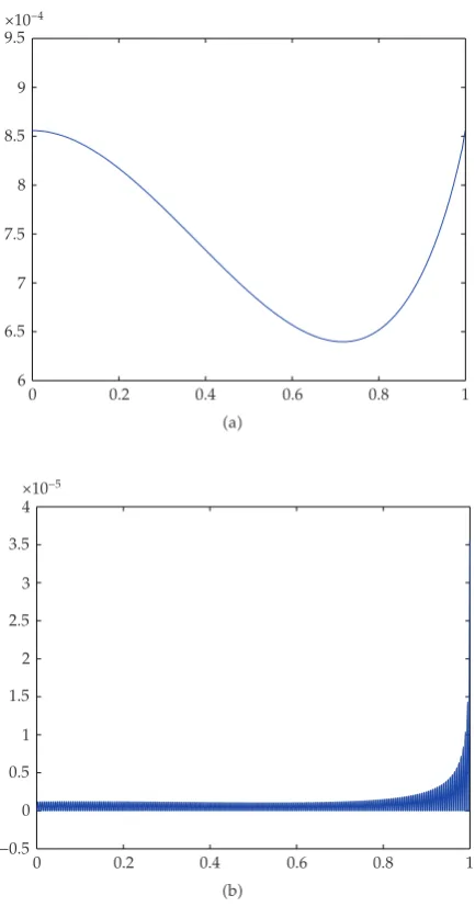
6 6.5 7 7.5 8 8.5 9 9.5 ×10⁻⁴
0 0.2 0.4 0.6 0.8 1
a
−0.5 0 0.5 1 1.5 2 2.5 3 3.5 4 ×10⁻⁵
0 0.2 0.4 0.6 0.8 1
b
Figure 5:Error estimateaand residualbfor5.43-5.1a,a1.
a0, T. Therefore, we can find a subsequence{um}such that{um}converges uniformly on
0, T, and{um}converges uniformly ona0, T. By the diagonalization theorem; see11, we
can find a subsequence{u}such that there existsu∈C0, T∩C10, Twith
lim
→ ∞ut utuniformly on0, T,
lim → ∞u
t utlocally uniformly on0, T.
5.34
−0.06 −0.04 −0.02 0 0.02 0.04 0.06 0.08
0 0.2 0.4 0.6 0.8 1
Figure 6:First derivative of the numerical solution to5.43-5.1awitha1.
convergence theorem yields
ut − T
t
a su
s fs, us, usds, t∈0, T. 5.35
Consequently,u∈AC1loc0, Tsatisfies equation5.1aa.e. on0, T. Moreover, due to5.22 and5.27, we have
A≤ut≤B fort∈0, T, ut≤ρ∗ fort∈0, T. 5.36
Hence4.1is satisfied. ApplyingTheorem 4.1, we conclude thatu∈AC10, Tandu0 0. Thereforeusatisfies the periodic conditions on0, T. Thusuis a solution of problem5.1a and5.1bandA≤u≤Bon0, T.
Example 5.4. LetT 1,k ∈N,ε±1,h∈Lp0,1for somep >1, andc0∈C0,1. Moreover,
lethbe nonnegative, and letc0be bounded on0,1. Then inTheorem 5.3the following class
of functionsfis covered:
ft, x, yht
x2k1εexync0tcos
|x|
5.37
for a.e.t∈0,1and allx, y∈R, providedn2m1 ifε1 andn1 ifε−1. In particular, fort∈0,1,x, y∈R
f1
t, x, y √1 1−t
x3exy5cos1
tcos
|x|
−0.939 −0.9385 −0.938 −0.9375 −0.937
0 0.01 0.02 0.03 0.04 0.05 0.06
n7
n8
n9
n10
a
−0.939 −0.9385 −0.938 −0.9375 −0.937
0.94 0.95 0.96 0.97 0.98 0.99 1
n7
n8
n9
n10
b
Figure 7:Numerical solutions of5.43-5.1aanda1 in the vicinity oft0aandt1b. The step size is decreasing according toh1/2n.
or
f2
t, x, y √1 1−t
x3−exycos1 tcos
|x|
. 5.39
1.55 1.6 1.65 1.7 1.75 1.8 1.85 1.9
0 0.2 0.4 0.6 0.8 1
a0.1
a0.5
a1
a2
a5
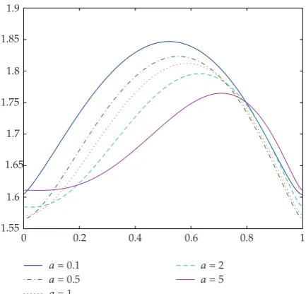
Figure 8:IllustratingTheorem 5.6: solutions of the boundary value problem5.44-5.1a. See graph legend for the values ofa.
Lemma 5.5Fredholm-type existence theorem. Letf satisfy2.2, let matricesB0, B1 ∈ R2×2,
vectorβ∈R2be given, and letc
1, c2∈L10, T. Let us denote byUt: ut, utT, and assume
that the linear homogeneous boundary value problem
uc1tuc2tu0, B0U0 B1UT 0 5.40
has only the trivial solution. Moreover, let us assume that there exists a functionm∈Lp0, Tsuch
that
ft, x, y≤mt for a.e. t∈0, Tand allx, y∈R. 5.41
Then the problem
uc1tuc2tuf
t, u, u, B0U0 B1UT β 5.42
has a solutionu∈AC10, T.
If we combine Theorems5.2and5.3, we obtain conditions sufficient for the solution of
5.1aand5.1bto be unique.
0.8 1 1.2 1.4 1.6 1.8 2 2.2 2.4 2.6 2.8 ×10⁻³
0 0.2 0.4 0.6 0.8 1
a
−2.5 −2 −1.5 −1 −0.5 0 0.5 ×10⁻³
0 0.2 0.4 0.6 0.8 1
b
Figure 9:Error estimateaand residualbfor5.44-5.1a,a1.
Example 5.7. Functions satisfying assumptions ofTheorem 5.6can have the form
ft, x, y √a 1−t
x3exy5t, 5.43
ft, x, y √a 1−t
x3−e−xy−16√t, 5.44
fort∈0,1, x, y∈R.
−0.8 −0.6 −0.4 −0.2 0 0.2 0.4 0.6
0 0.2 0.4 0.6 0.8 1
Figure 10:First derivative of the numerical solution to5.44-5.1awitha1.
Table 1:Estimated convergence order for the periodic boundary value problem5.43-5.1aanda1.
i Error estimate Conv. order
1 5.042446e–003 —
2 2.850171e–003 0.823075
3 1.681410e–003 0.761377
4 1.029876e–003 0.707200
5 6.514046e–004 0.660845
6 4.231359e–004 0.622433
7 2.807926e–004 0.591616
8 1.894611e–004 0.567604
9 1.294654e–004 0.549335
10 8.930836e–005 0.535699
obtained from the substitution of the numerical solution into the differential equation. Both quantities are rather small and indicate that we have found a solution to the analytical problem5.43-5.1a.
We now pose that question about the values of the first derivative at the end points of the interval of integration,t0 andt1. According to the theory, it holds thatu0 u1 0. Therefore, we approximate the values of the first derivative of the numerical solution and show these values inFigure 6. One can see that indeedu0≈0, u1≈0. Also, to support this observation, we plotted inFigure 7the numerical solutions obtained for the step sizeh tending to zero, or equivalently, grids becoming finer.
We finally observe experimentally the order of convergence of the numerical method
collocation. Clearly, we do not expect very hight order to hold, since the analytical solution has nonsmooth higher derivatives. However, the method is convergent and, according to Table 1, we observe that its order tends to 1/2.
1.564 1.566 1.568 1.57 1.572 1.574 1.576 1.578 1.58 1.582 1.584
0 0.01 0.02 0.03 0.04 0.05 0.06
n7
n8
n9
n10
a
1.566 1.568 1.57 1.572 1.574 1.576 1.578 1.58 1.582 1.584 1.586
0.94 0.95 0.96 0.97 0.98 0.99 1
n7
n8
n9
n10
b
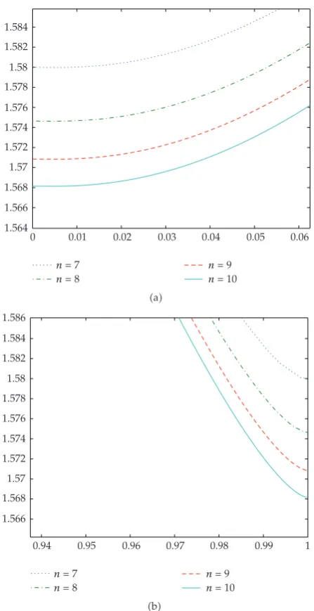
Figure 11:Numerical solutions of5.44-5.1aanda1 in the vicinity oft0aandt1b. The step size is decreasing according toh1/2n.
Acknowledgments
This research was supported by the Council of Czech Goverment MSM6198959214 and by the Grant no. A100190703 of the Grant Agency of the Academy of Sciences of the Czech Republic.
References
2 R. P. Agarwal and D. O’Regan, “Singular problems arising in circular membrane theory,”Dynamics of Continuous, Discrete & Impulsive Systems. Series A, vol. 10, no. 6, pp. 965–972, 2003.
3 J. V. Baxley, “A singular nonlinear boundary value problem: membrane response of a spherical cap,”
SIAM Journal on Applied Mathematics, vol. 48, no. 3, pp. 497–505, 1988.
4 J. V. Baxley and G. S. Gersdorff, “Singular reaction-diffusion boundary value problems,”Journal of Differential Equations, vol. 115, no. 2, pp. 441–457, 1995.
5 A. Constantin, “Sur un probleme aux limites en mecanique non lineaire,”Comptes Rendus de l’Acad´emie des Sciences. S´erie I, vol. 320, no. 12, pp. 1465–1468, 1995.
6 R. W. Dickey, “Rotationally symmetric solutions for shallow membrane caps,” Quarterly of Applied Mathematics, vol. 47, no. 3, pp. 571–581, 1989.
7 R. W. Dickey, “The plane circular elastic surface under normal pressure,”Archive for Rational Mechanics and Analysis, vol. 26, no. 3, pp. 219–236, 1967.
8 V. Hlavacek, M. Marek, and M. Kubicek, “Modelling of chemical reactors-X. Multiple solutions of enthalpy and mass balances for a catalytic reaction within a porous catalyst particle,” Chemical Engineering Science, vol. 23, no. 9, pp. 1083–1097, 1968.
9 K. N. Johnson, “Circularly symmetric deformation of shallow elastic membrane caps,”Quarterly of Applied Mathematics, vol. 55, no. 3, pp. 537–550, 1997.
10 I. Rach ˚unkov´a, O. Koch, G. Pulverer, and E. Weinm ¨uller, “On a singular boundary value problem arising in the theory of shallow membrane caps,”Journal of Mathematical Analysis and Applications, vol. 332, no. 1, pp. 523–541, 2007.
11 I. Rach ˚unkov´a, S. Stanˇek, and M. Tvrd ´y, “Singularities and Laplacians in boundary value problems for nonlinear ordinary differential equations,” in Handbook of Differential Equations: Ordinary Differential Equations, A. Ca ˇnada, P. Dr´abek, and A. Fonda, Eds., vol. 3 ofHandbook of Differential Equations, pp. 607–722, Elsevier, Amsterdam, The Netherlands, 2006.
12 J. Y. Shin, “A singular nonlinear differential equation arising in the Homann flow,” Journal of Mathematical Analysis and Applications, vol. 212, no. 2, pp. 443–451, 1997.
13 E. Weinm ¨uller, “On the boundary value problem for systems of ordinary second-order differential equations with a singularity of the first kind,”SIAM Journal on Mathematical Analysis, vol. 15, no. 2, pp. 287–307, 1984.
14 O. Koch, “Asymptotically correct error estimation for collocation methods applied to singular boundary value problems,”Numerische Mathematik, vol. 101, no. 1, pp. 143–164, 2005.
15 F. R. de Hoog and R. Weiss, “Difference methods for boundary value problems with a singularity of the first kind,”SIAM Journal on Numerical Analysis, vol. 13, no. 5, pp. 775–813, 1976.
16 F. R. de Hoog and R. Weiss, “The numerical solution of boundary value problems with an essential singularity,”SIAM Journal on Numerical Analysis, vol. 16, no. 4, pp. 637–669, 1979.
17 G. Kitzhofer,Numerical treatment of implicit singular BVPs, Ph.D. thesis, Institute for Analysis and Scientific Computing, Vienna University of Technology, Vienna, Austria, 2005, in prepartion.
18 I. Rach ˚unkov´a, G. Pulverer, and E. Weinm ¨uller, “A unified approach to singular problems arising in the membran theory,” to appear inApplications of Mathematics.
19 I. T. Kiguradze and B. L. Shekhter, “Singular boundary value problems for second-order ordinary differential equations,” in Current Problems in Mathematics. Newest Results, Vol. 30 (Russian), Itogi Nauki i Tekhniki, pp. 105–201, Akad. Nauk SSSR Vsesoyuz. Inst. Nauchn. i Tekhn. Inform., Moscow, Russia, 1987, translated inJournal of Soviet Mathematics, vol. 43, no. 2, pp. 2340–2417, 1988.
20 A. Lasota, “Sur les probl`emes lin´eaires aux limites pour un syst`eme d’´equations diff´erentielles ordinaires,”Bulletin de l’Acad´emie Polonaise des Sciences. S´erie des Sciences Math´ematiques, Astronomiques et Physiques, vol. 10, pp. 565–570, 1962.