A Bias Correction for the Minimum Error Rate in
Cross-validation
Ryan J. Tibshirani∗ Robert Tibshirani†
Abstract
Tuning parameters in supervised learning problems are often esti-mated by cross-validation. The minimum value of the cross-validation error can be biased downward as an estimate of the test error at that same value of the tuning parameter. We propose a simple method for the estimation of this bias that uses information from the cross-validation process. As a result, it requires essentially no additional computation. We apply our bias estimate to a number of popular clas-sifiers in various settings, and examine its performance.
Key words: cross-validation, prediction error estimation, optimism es-timation
1
Introduction
Cross-validation is widely used in regression and classification problems to choose the value of a “tuning parameter” in a prediction model. By training and testing the model on separate subsets of the data, we get an idea of the model’s prediction strength as a function of the tuning parameter, and we choose the parameter value to minimize the CV error curve. This estimate admits many nice properties (see Stone 1997 for a discussion of asymptotic consistency and efficiency) and works well in practice.
However, the minimum CV error itself tends to be too optimistic as an estimate of true prediction error. Many have noticed this downward bias in the minimum error rate. Breiman, Friedman, Olshen & Stone (1984)
∗
Dept. of Statistics, Stanford University, [email protected]. Supported by a Na-tional Science Foundation Vertical Integration of Graduate Research and Education fel-lowship.
†Dept. of Statistics, Stanford University, [email protected]. Supported in part by
Na-tional Science Foundation Grant DMS-9971405 and NaNa-tional Institutes of Health Contract N01-HV-28183.
acknowledge this bias in the context of classification and regression trees. Efron (2008) discusses this problem in the setting p ≫ n, and employs an empirical Bayes method, which does not involve cross-validation in the choice of tuning parameters, to avoid such a bias. However, the proposed al-gorithm requires an initial choice for a “target error rate”, which complicates matters by introducing another tuning parameter. Varma & Simon (2006) suggest a method using “nested” cross-validation to estimate the true error rate. This essentially amounts to doing a cross-validation procedure for ev-ery data point, and is hence impractical in settings where cross-validation is computationally expensive.
We propose a bias correction for the minimum CV error rate in K-fold cross-validation. It is computed directly from the individual error curves from each fold, and hence does not require a significant amount of additional computation.
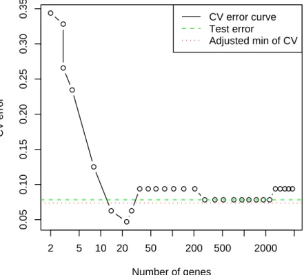
Figure 1 shows an example. The data come from the laboratory of Dr. Pat Brown of Stanford, consisting of gene expression measurements over 4718 genes on 128 patient samples, 88 from healthy tissues and 30 from CNS tumors. We randomly divided the data in half, into training and test samples, and applied the nearest shrunken centroids classifier (Tibshirani, Hastie, Narasimhan & Chu 2001) with 10-fold cross-validation, using the pamr package in the R language. The figure shows the CV curve, with its minimum at 23 genes, achieving a CV error rate of 4.7%. The test error at 23 genes is 8%. The estimate of the CV bias, using the method described in this in paper, is 2.7%, yielding an adjusted error of 4.7 + 2.7 = 7.4%. Over 100 repeats of this experiment, the average test error was 7.8%, and the average adjusted CV error was 7.3%.
In this paper we study the CV bias problem and examine the accuracy of our proposed adjustment on simulated data. These examples suggest that the bias is larger when the signal-to-noise ratio is lower, a fact also noted by Efron (2008). We also provide a short theoretical section examining the expectation of the bias when there is no signal at all.
2
Model Selection Using Cross-Validation
Suppose we observe n independent and identically distributed points (xi, yi), where xi = (xi1, . . . , xip) is a vector of predictors, and yi is a response (this can be real-valued or discrete). From this “training” data we estimate a prediction model ˆf(x) for y, and we have a loss function L(y, ˆf(x)) that
2 5 10 20 50 200 500 2000 0.05 0.10 0.15 0.20 0.25 0.30 0.35 Number of genes CV error CV error curve Test error Adjusted min of CV
Figure 1: Brown microarray cancer data: the CV error curve is minimized at 23 genes, achieving a CV error of 0.047. Meanwhile, the test error at 23 genes is 0.08, drawn as a dashed line. The proposed bias estimate is 0.027, giving an adjusted error of 0.047 + 0.027 = 0.074, drawn as a dotted line.
measures the error between y and ˆf(x). Typically this is L(y, ˆf(x)) = (y − ˆf(x))2
squared error for regression, and
L(y, ˆf(x)) = 1{y 6= ˆf(x)} 0-1 loss for classification.
An important quantity is the expected prediction error E[L(y0, ˆf(x0))] (also called expected test error). This is the expected value of the loss when predicting an independent data point (x0, y0), drawn from the same distribution as our training data. The expectation is over all that is random (namely, the model ˆf and the test point (x0, y0)).
Suppose that our prediction model depends on a parameter θ, that is ˆ
f(x) = ˆf(x, θ). We want to select θ based on the training set (xi, yi), i = 1, . . . , n, in order to minimize the expected prediction error.
One of the simplest and most popular methods for doing this is K-fold cross-validation. We first split our data (xi, yi) into K equal parts. Then for each k = 1, . . . , K, we remove the kth part from our data set and fit a model ˆf−k(x, θ). Let Ck be the indices of observations in the kth fold. The cross-validation estimate of expected test error is
CV(θ) = 1 n K X k=1 X i∈Ck L(yi, ˆf−k(xi, θ)). (1)
Recall that ˆf−k(xi, θ) is a function of θ, so we compute CV(θ) over a grid of parameter values θ1, . . . , θt, and choose the minimizer ˆθto be our parameter estimate. We call CV(θ) the “CV error curve”.
3
Bias Correction
We would like to estimate the expected test error using ˆf(x, ˆθ), namely Err = E[L(y0, ˆf(x0, ˆθ))].
The naive estimate is CV(ˆθ), having bias
Let nk be the number of observations in the kth fold, and define ek(θ) = 1 nk X i∈Ck L(yi, ˆf−k(xi, θ))
This is the error curve computed from the predictions in the kth fold. Our estimate uses the difference between the value of ek at ˆθ and its minimum to mimic the bias in cross-validation. Specifically, we propose the following estimate: d Bias = 1 K K X k=1 [ek(ˆθ) − ek(ˆθk)] (3)
where ˆθkis the minimizer of ek(θ). Note that this estimate uses only quanti-ties that have already been computed for the CV estimate (1), and requires no new model fitting. Since dBias is a mean over K folds, we can also use the standard error of the mean as an approximate estimate for its standard deviation.
The adjusted estimate of test error is CV(ˆθ) + dBias. Note that if the fold sizes are equal, then CV(ˆθ) = K1 PKk=1ek(ˆθ) and the adjusted estimate of test error is CV(ˆθ) + dBias = 2CV(ˆθ) − 1 K K X k=1 ek(ˆθk).
The intuitive motivation for the estimate dBias is as follows: first, ek(ˆθk) ≈ CV(ˆθ) since both are error curves evaluated at their minima; the latter uses all K folds while the former uses just fold k. Second, for fixed θ, cross-validation error estimates the expected test error, so that ek(θ) ≈ E[L(y, ˆf(x, θ))]. Thus ek(ˆθ) ≈ Err.
The second analogy is not perfect: Err = E[L(y, ˆf(x, ˆθ))], where (x, y) is stochastically independent of the training data, and hence of ˆθ. In con-trast, the terms in ek(ˆθ) are L(yi, ˆf−k(xi, ˆθ)), i ∈ Ck; here (xi, yi) has some dependence on ˆθsince ˆθis chosen to minimize the validation error across all folds, including the kth one. To remove this dependence, one would have to carry out a new cross-validation for each of the K original folds, which is much more computationally expensive.
There is a similarity between the bias estimate in (3) and bootstrap estimates of bias (Efron 1979, Efron & Tibshirani 1993). Suppose that we have data z = (z1, z2, . . . zn) and a statistic s(z). Let z∗1, z∗2, . . . z∗B be
bootstrap samples each of size n drawn with replacement from z. Then the bootstrap estimate of bias is
d Biasboot= 1 B B X b=1 [s(z∗b) − s(z)]. (4)
Suppose that s(z) is a functional statistic and hence can be written as t( ˆF), where ˆF is the empirical distribution function. ThenBiasdboot approximates EF[t( ˆF)] − t(F ), the expected bias in the original statistic as an estimate of the true parameter t(F ).
Now to estimate the quantity Bias in (2), we could apply the bootstrap estimate in (4). This would entail drawing bootstrap samples and computing a new cross-validation curve from each sample. Then we would compute the difference between the minimum of the curve and the value of curve at the training set minimizer. In detail, let CV(z∗, ˆθ(˜z)) be the value of the cross-validation curve computed on the dataset z∗ and evaluated at ˆθ(˜z), the minimizer for the CV curve computed on dataset ˜z. Then the bootstrap estimate of bias can be expressed as
1 B B X b=1 [CV(z∗b, ˆθ(z)) − CV(z∗b, ˆθ(z∗b))]. (5) The computation of this estimate is expensive, requiring B K-fold cross-validations, where B is typically 100 or more. The estimate in dBias in (3) finesses this by using the original cross-validation folds to approximate the bias in place of the bootstrap samples.
In the next section, we examine the performance of our estimate in var-ious contexts.
4
Application to Simulated Data
We carried out a simulation study to examine the size of the CV bias, and the accuracy of our proposed adjustment (3). The data were generated as standard Gaussian in two settings: p < n (n = 400, p = 100) and p ≫ n (n = 40, p = 1000). There were two classes of equal size. For each of these we created two settings: “no signal”, in which the class labels were independent of the features, and “signal”, where the mean of the first 10% of the features were shifted to be 0.5 units higher in class 2.
(lin-p < n
Method Min CV error Test error Adjusted CV error No signal LDA 0.503 (0.003) 0.5 0.503 (0.003) SVM 0.485 (0.003) 0.5 0.511 (0.004) CART 0.474 (0.003) 0.5 0.510 (0.004) KNN 0.473 (0.002) 0.5 0.524 (0.003) GBM 0.475 (0.003) 0.5 0.520 (0.003) Signal LDA 0.290 (0.003) 0.284 (0.001) 0.290 (0.003) SVM 0.257 (0.003) 0.260 (0.001) 0.279 (0.003) CART 0.356 (0.003) 0.378 (0.002) 0.384 (0.003) KNN 0.291 (0.003) 0.284 (0.002) 0.305 (0.004) GBM 0.269 (0.002) 0.272 (0.002) 0.288 (0.003) p≫ n
Method Min CV error Test error Adjusted CV error No signal NSC 0.384 (0.009) 0.5 0.511 (0.012) SVM 0.475 (0.009) 0.5 0.498 (0.010) CART 0.498 (0.011) 0.5 0.500 (0.011) KNN 0.430 (0.007) 0.5 0.577 (0.009) GBM 0.432 (0.010) 0.5 0.552 (0.012) Signal NSC 0.106 (0.006) 0.136 (0.004) 0.152 (0.008) SVM 0.142 (0.007) 0.138 (0.003) 0.157 (0.008) CART 0.432 (0.012) 0.432 (0.004) 0.437 (0.012) KNN 0.200 (0.007) 0.251 (0.005) 0.297 (0.010) GBM 0.233 (0.008) 0.276 (0.006) 0.307 (0.010)
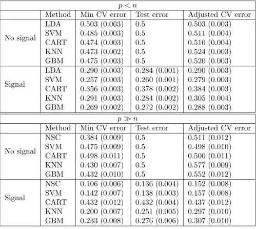
Table 1: Results for proposed bias correction for the minimum CV error, using 10-fold cross-validation. Shown are mean and standard error over 100 simulations, for five different classifiers.
(classification and regression trees), KNN (K-nearest neighbors), and GBM (gradient boosting machines). In the p ≫ n setting, the LDA solution is not of full rank, so we used diagonal linear discriminant analysis with soft-thresholding of the centroids, known as nearest shrunken centroids (NSC). Table 1 shows the mean of the test error, minimum CV error (using 10-fold CV), true bias, and estimated bias, over 100 simulations. The standard errors are given in brackets.
We see that the bias tends to larger in the “no signal” case, and varies significantly depending on the classifier. And it seems to be sizable only when p ≫ n. The bias adjustment is quite accurate in most cases, except for the KNN and GBM classifiers when p ≫ N , when it is too large. With only 40 observations, 10-fold CV has just four observations in each fold, and this may cause erratic behavior for these highly non-linear classifiers. Table
Classifier Setting Min CV error Test error Adjusted CV error KNN No signal 0.430 (0.007) 0.5 0.524 (0.009) KNN Signal 0.213 (0.007) 0.253 (0.005) 0.281 (0.009) GBM No signal 0.425 (0.008) 0.5 0.511 (0.010) GBM Signal 0.265 (0.008) 0.289 (0.007) 0.325 (0.010)
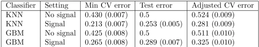
Table 2: Results for KNN and GBM when p ≫ N , with 5-fold cross-validation.
2 shows the results for KNN and GBM when p ≫ N , with 5-fold CV. Here the bias estimate is more accurate, but is still slightly too large.
5
Nonnegativity of the Bias
Recall section 3, where we introduced Bias = Err − CV(ˆθ), and our estimate d
Bias. It follows from the definition that dBias ≥ 0 always. We show that for classification problems, E[Bias] ≥ 0 when there is no signal.
Theorem 1. Suppose that there is no true signal, so that y0 is stochastically
independent of x0. Suppose also that we are in the classification setting,
and y0 = 1, . . . G with equal probability. Finally suppose that the loss is 0-1, L(y, ˆf(x)) = 1{y 6= ˆf(x)}. Then E[CV(ˆθ)] ≤ Err.
Proof. The proof is quite straightforward. Well Err = 1 − P(y0= ˆf(x0, ˆθ)), where ˆf( · , ˆθ) is fit on the training examples (x1, y1), . . . (xn, yn). Suppose that marginally P( ˆf(x0, ˆθ) = j) = pj, for j = 1, . . . G. Then by independence
P(y0 = ˆf(x0, ˆθ)) = X j P(y0 = ˆf(x0, ˆθ) = j) = X j 1 Gpj = 1 G,
so Err = G−1G . By the same argument, E[CV(θ)] = G−1G for any fixed θ. Therefore
E[CV(ˆθ)] = E[miniCV(θi)] ≤ E[CV(θ1)] = G− 1
G , which completes the proof.
Now suppose that there is no signal and we are in the regression setting with squared error loss, L(y, ˆf(x)) = (y − ˆf(x))2
. We conjecture that indeed E[CV(ˆθ)] ≤ Err for a fairly general class of models ˆf.
on the test set in order to determine a value for θ (just treating the test data like it were training data). That is, define
g CV(θ) = 1 n K X k=1 X i∈Ck (˜yi− ˜f−k(˜xi, θ)) 2 ,
where ˜f−k is fit on all test examples (˜xi,y˜i) except those in the kth fold. Let ˜θ be the minimizer of gCV(θ) over θ1, . . . θt. Then
E[CV(ˆθ)] = E[gCV(˜θ)] ≤ E[gCV(ˆθ)],
where the first step is true by symmetry, and the second is true by defi-nition of ˜θ. But (assuming for notational simplicity that 1 ∈ C1) we have E[gCV(ˆθ)] = E[(˜y1− ˜f−1(˜x1, ˆθ))2]. Further, we conjecture that
E[(˜y1− ˜f−1(˜x1, ˆθ)) 2
] = E[(˜y1− ˆf−1(˜x1, ˆθ)) 2
]. (6)
Intuitively: since there is no signal, ˜f( · , ˆθ) and ˆf( · , ˆθ) should predict equally well against a new example (˜x1,y˜1), because ˆθ should not have any real relation to predictive strength.
For example, if we are doing ridge regression with p = 1 and K = n (leave-one-out CV), and we assume that each xi= ˜xi is fixed (nonrandom), then we can write out the model ˆf−k( · , θ) explicitly. In this case, statement (6) can be reduced to:
E[y1|ˆθ] = E[y1], E[y 2
1|ˆθ] = E[y 2
1], and E[y1y2|ˆθ] = E[y1]E[y2]. In words: the mean and variance of y1 are unchanged by conditioning on ˆθ, and y1, y2 are conditionally independent given ˆθ. These certainly seem true when looking at simulations, but are hard to prove rigorously because of the complicated relationship between the yi and ˆθ.
Similarly, we conjecture that E[(˜y1− ˆf−1(˜x1, ˆθ))
2
] = E[(˜y1− ˆf(˜x1, ˆθ)) 2
], (7)
because there is no signal. If we could show (6) and (7), then we would have E[CV(ˆθ)] ≤ E[(˜y1− ˆf(˜x1, ˆθ))2] = Err.
6
Discussion
We have proposed a simple estimate of the bias of the minimum error rate in cross-validation. It is easy to compute, requiring essentially no additional
computation after the initial cross-validation. Our studies indicate that it is reasonably accurate in general. We also found that the bias itself is only an issue when p ≫ N and its magnitude varies considerably depending on the classifier. For this reason, it can be misleading to compare the CV error rates when choosing between models (e.g. choosing between NSC and SVM); in this situation the bias estimate is very important.
Acknowledgements: The authors would like to thank the Editor for helpful comments that led to improvements in the paper.
References
Breiman, L., Friedman, J., Olshen, R. & Stone, C. (1984), Classification
and Regression Trees, Wadsworth.
Efron, B. (1979), ‘Bootstrap methods: another look at the jackknife’, Annals
of Statistics 7, 1–26.
Efron, B. (2008), Empirical bayes estimates for large-scale prediction prob-lems.
URL: http: // www-stat. stanford. edu/ ~ ckirby/ brad/ papers/
2008EBestimates. pdf
Efron, B. & Tibshirani, R. (1993), An Introduction to the Bootstrap, Chap-man and Hall, London.
Stone, M. (1977), ‘Asymptotics for and against cross-validation’, Biometrika 64(1), 29–35.
Tibshirani, R., Hastie, T., Narasimhan, B. & Chu, G. (2001), ‘Diagnosis of multiple cancer types by shrunken centroids of gene expression’, Proc.
Natl. Acad. Sci. 99, 6567–6572.
Varma, S. & Simon, R. (2006), ‘Bias in error estimation when using cross-validation for model selection’, BMC Bioinformatics 91(7).