Yang, Zhijing and Cao, Faxian and Ren, Jinchang and Ling, Wing-Kuen
(2018) Convolutional neural network extreme learning machine
(CNN-ELM) for effective classification of hyperspectral images. Journal of
Applied Remote Sensing. ISSN 1931-3195 (In Press) ,
This version is available at https://strathprints.strath.ac.uk/64512/
Strathprints is designed to allow users to access the research output of the University of Strathclyde. Unless otherwise explicitly stated on the manuscript, Copyright © and Moral Rights for the papers on this site are retained by the individual authors and/or other copyright owners. Please check the manuscript for details of any other licences that may have been applied. You may not engage in further distribution of the material for any profitmaking activities or any commercial gain. You may freely distribute both the url (https://strathprints.strath.ac.uk/) and the content of this paper for research or private study, educational, or not-for-profit purposes without prior permission or charge.
Any correspondence concerning this service should be sent to the Strathprints administrator: [email protected]
The Strathprints institutional repository (https://strathprints.strath.ac.uk) is a digital archive of University of Strathclyde research outputs. It has been developed to disseminate open access research outputs, expose data about those outputs, and enable the
Hyperspectral Image Classification with A Convolutional Neural
Network-Extreme Learning Machine (CNN-ELM) Approach
Zhijing Yang1, Faxian Cao1, Jinchang Ren2*, Wing-Kuen Ling1
1
School of Information Engineering, Guangdong University of Technology, Guangzhou, 510006, China
2
Department of Electronic and Electrical Engineering, University of Strathclyde, Glasgow, G1 1XW, UK
*
Email: [email protected]
Abstract—Due to its excellent performance in terms of fast implementation, strong generalization capability and straightforward solution, extreme learning machine (ELM) has attracted increasingly attentions in pattern recognition such as face recognition and hyperspectral image (HSI) classification. However, the performance of ELM for HSI classification remains a challenging problem especially in effective extraction of the featured information from the massive volume of data. To this end, we propose in this paper a new method to combine Convolutional neural network (CNN) with ELM (CNN-ELM) for HSI classification. As CNN has been successfully applied for feature extraction in different applications, the combined CNN-ELM approach aims to take advantages of these two techniques for improved classification of HSI. By preserving the spatial features whilst reconstructing the spectral features of HSI, the proposed CNN-ELM method can significantly improve the accuracy of HSI classification without increasing the computational complexity. Comprehensive experiments using three publicly available HSI data sets, Pavia University, Pavia center, and Salinas have fully validated the improved performance of the proposed method when benchmarking with several state-of-the-art approaches.
Keywords—Hyperspectral image (HSI) classification, Convolutional neural network (CNN), Extreme Learning Machine (ELM).
I. Introduction
With spectral information in hundreds of continuous narrow bands and spatial information acquired simultaneously, hyperspectral imaging has facilitated a number of applications especially in remote sensing
earth observation. As the spectral profiles can reflect certain physical (i.e. moisture/temperature) or chemical differences of the objects, this has been widely used in land mapping for classification of the images. Although HSI data classification is conceptually similar to image labeling in computer vision [1], one fundamental challenge here is the curse of dimensionality caused by limited labeled data samples (in spatial domain) but too many spectral bands (feature dimensions) [2, 3].
To tackle this problem, a number of techniques have been proposed for feature extraction and dimensionality reduction [9, 13], such as principal component analysis (PCA) [10], singular spectrum analysis (SSA) [5-7], Low-Rank Representation [8], and segmented auto-encoder [12]. For data classification, typical approaches include support vector machine (SVM) [4], multi-kernel classification [11], k-nearest-neighbors (k-NN) [14] and multinomial logistic regression [15, 16] (MLR) et al. Among these approaches, spatial-spectral analysis becomes a trend as it takes information in both spatial domain and spectral domain into consideration. Whilst spectral information measures the physical/chemical characteristics, it is the spatial structuring information that groups pixels into objects. Therefore, fusion of these two modalities of information is essential for classification of HSI data.
For effective spatial-spectral analysis of HSI, convolutional neural network (CNN) based deep learning is employed for its success in feature extraction and extraction of the hidden structures of the data [21]. As one of the most popularly used model in deep learning, CNN can exploit spatially local correlation by enforcing a local connectivity pattern between neurons of adjacent layers [22-26]. Although CNN has already been successfully applied for HSI classification [27-29], the training process is over complicated due to the lengthy iterations over the high data volume. For practical applications especially with airborne or satellite based systems, the computational cost needs be cut down to the meet the requirement for real-time data analysis.
for hyperspectral image classification. Rather using a lengthy process for iterative feature extraction, we only apply CNN in one iteration for training, followed by ELM for data classification under significantly reduced time for feature extraction. As a single-hidden layer feedforward neural network, ELM has been successfully applied in a number of application areas for merits in terms of fast implementation, straightforward solution and strong generalization capability [17-19]. As a result, the combination of these two methods is expected to produce much improved data classification results in our proposed CNN-ELM approach.
The main contributions of the proposed CNN-ELM approach can be highlighted as follows. First, the combination itself is rare, especially for HSI classification with CNN used for feature extraction and ELM for data classification. Second, the proposed method can not only reconstructs the spectral features but also preserve the spatial information. Third, the concept to have CNN only applied for one iteration has significantly reduced the computational cost whilst still improved the classification accuracy. The experiment results on three well-known publicly available HSI data sets, Pavia University, Pavia center, and Salinas, have validated the efficacy of the proposed approach when benchmarking with several the-state-of-art techniques.
The remainder of this paper is organized as follows. Section �� introduces briefly the background knowledge of ELM and CNN. Section ��� discusses in detail the proposed CNN-ELM approach in three steps, i.e. normalization, CNN based spectral feature reconstruction and ELM based classification. Experimental results and analysis are presented in Section IV, followed by some concluding remarks drawn in Section ‡.
II. Introduction of ELM and CNN for Data Classification in HSI
In this section, the background knowledge of CNN and ELM is presented. Discussions are followed to show how they can be applied in HSIs for data classification.
A. Background introduction of ELM
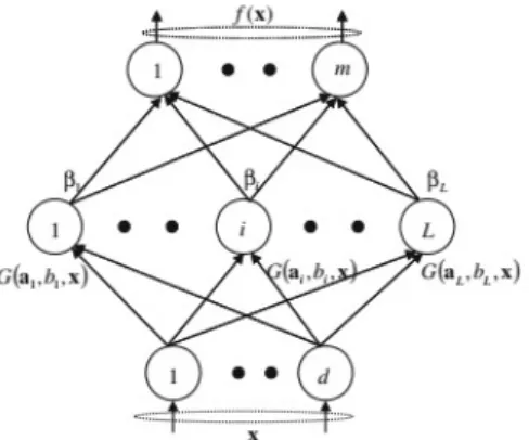
pixels and each sample is a d-dimension vector, we also define y y y R as the desired output of M different labels for the N samples. As shown in Fig. 1, ELM is a single-hidden layer feedforward neural network, and an ELM with L hidden nodes can be modeled as [30]:
g w x b (1)
where T is the transpose operation, w w w and are respectively the weight vector and the bias connecting the input layer and hidden layer of the i-th sample of his. In addition, is the ouput weight vector of i-th sample of his, and g is the activation function.
Fig. 1. The architecture of an ELM.
For data classification, there are three key steps in ELM as detailed below.
Step1: Assign random inputs for the weight vector w and the bias b, where i N; Step2: Using (1) to calculate the output matrix of the hidden layer G
where � w w w x x x b b b
g w x b g w x b
g w x b g w x b (2) Step 3: Calculate the output weight matrix by
(3) where denotes Moore-Penrose generalized inverse of matrix G, y represent the desired output in (1).
bias of ELM are randomly generated and The output weight matrix can be computed as � , so the time-consuming can be greatly reduce.
B. Background introduction of CNN
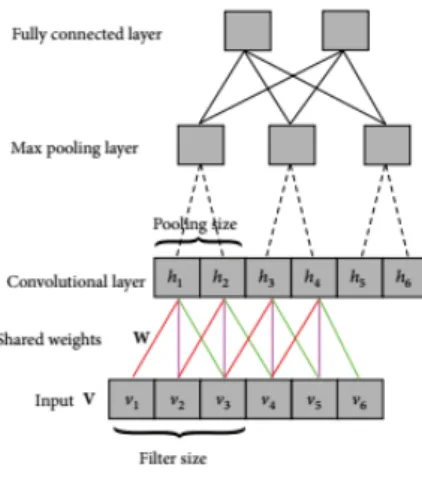
CNN is considered to be one of the relatively successful machine learning methods because of its good performance. As shown in Fig. 1, a typical CNN consists of several layers [22, 31]. The first layer is the input layer, while the second and third layers are the convolution layer and the max pooling layer, respectively. The convolution layer convolutes the input data Vto form the feature map to reduce the training parameters. That is to say, each hidden activation function of CNN is computed by multiplying a small local input with the weights
W. The neurons belonging to same layer share the same weights, which can be describe as follows: (5)
where is the bias of the convolutional layer. The max pooling layer partitions the feature map from convolutional layer into a set of non-overlapping windows and outputs the maximum value. The final layer is a fully connected layer which outputs the classification results.
Fig. 2. A typical architecture of CNN consists of input layer, convolutional layer, max pooling layer and fully connected layer.
C. Adapting CNN and ELM in HSI
promising method with the following advantages [20]. Firstly, it has a simpler structure and higher generalization performance than SVM and most others. Secondly, it has a very high computational efficiency for greatly shortened training time. Thirdly, it needs no tuning of additional parameters when the network structure is set. Fourthly, there are many available piecewise continual functions which can be used as the activation function, such as sine function, radial basis function and sigmoid function, etc. As a result, ELM has been successfully applied in many applications [20]. However, the classification results are not high when applying ELM directly to HSI. The reason of low recognition rate mainly is that the ELM cannot catch the depth features of HSI. For example, as reported in [32], the overall classification accuracy of ELM for Pavia University data sets is only 79.58%. Therefore it is a critical problem how to maintain fast speed of ELM and improve the accuracy for HSI classification.
As mentioned above, CNN can extract the spectral features of depth of HSI data very well. So we use CNN to extract the depth feature of HSI, then the reconstructed pixels of HSI are used as the input of ELM. The combination of these two methods is expected to obtain good classification results and maintain the fast speed for HIS classification.
III The Proposed CNN-ELM Approach
The proposed method can be divided into three parts: normalization, spectral feature reconstruction using CNN, and classification using ELM.
A. Normalization
Let x be a HSI data that has N samples and L feature. Normalization is a preprocessing process that it makes the HSI data remain in the range of [0,1] by the following formula:
where is one pixel of the HSI data, max() gets the largest one of all the data.
B. Spectral feature reconstruction using CNN
In order to maintain the high speed of the algorithm, we let CNN iterate only one time to reduce the time-consuming. The hierarchical structure of CNN has been shown to be the most successful and efficient method to learn visual features. HSI data have hundreds of spectral bands so that we can think of the spectral feature of pixels as a two-dimensional curve. We use CNN to extract the spectral feature of the depth of the pixel to reconstruct the spectral feature, and then improve classification accuracy of ELM with little time-consuming.
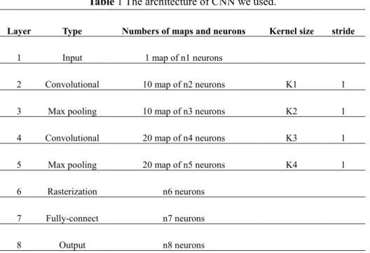
Table 1 The architecture of CNN we used.
Layer Type Numbers of maps and neurons Kernel size stride
1 Input 1 map of n1 neurons
2 Convolutional 10 map of n2 neurons K1 1
3 Max pooling 10 map of n3 neurons K2 1
4 Convolutional 20 map of n4 neurons K3 1
5 Max pooling 20 map of n5 neurons K4 1
6 Rasterization n6 neurons
7 Fully-connect n7 neurons
8 Output n8 neurons
As show in Table 1, CNN consists of eight layers. The first layer is the input layer which represents the spectral vector of one pixel of HSI data set. The second and third layers are the convolution layer and the max pooling layer, respectively. The fourth layer and the fifth layer are also convolution and max pooling layer. The data from convolutional layer after max pooling operation is a series of feature map, but the input received by the multi-layer perceptron is a vector. So the elements in these feature maps should be arranged in a vector. The
sixth layer is the rasterization layer which is a fully connected layer, followed by another fully connected layer, and then the final layer is the output layer. The output layer of CNN is just used for training. The purpose is to update the weights and bias for back propagation, which would allow deeper features to be extracted. We will not use the output layer when we test our labeled sample. is assumed to represent all training parameters, ={ } and i=2,3,4,5,6,7,8 where is the parameters set between the (i-1)-th and the i-th layers.
Assuming is the input of the i-th layer and the output of the th (i+1)-th layer, we can compute by the following formula:
(7) where
(8)
and is transpose operation, and is the weight matrix and bias of the ith layer acting on the input data, respectively.
For the output layer, we use softmax function as the activation function, which is defined as:
y (9)
The back propagation updates the weights according to the error until the error is acceptable. The error is the deviation between the actual response the training sample in the forward propagation phase and the target output corresponding to the sample. The training parameters are updated by minimizing the loss function which is achieved by gradient descent. The loss function in our work is defined as follow:
� log (10)
where p is the total number of training samples, � and are the desired output and the actual output of the
j-th sample, respectively. The probability value of the desired output of the j-th sample is 1, and the probability value of the others is 0. The expression if j is equal to the desired output of the ith
training sample, and otherwise its value is equal to 0. The training parameters are update with the following equation:
(11) where is the learning factor, is set to be 0.05 in our experiment, and
(12) and
(13)
C. Classification using ELM
As mentioned above, when applying to HSI data set, ELM can’t extract the spectral feature of depth. It causes low recognition rate. To improve the accuracy, we use CNN to reconstruct the spectral features. Then the spectral features of depth are used as the input of ELM. Let be the reconstructed spectral feature data sets, i.e., every pixel of HSI is reconstructed to be Q-dimensions,
be the corresponding target label, L be the hidden neuron numbers and be the activation function of hidden layer, then the process of classification by ELM can be described as follow:
Step1: Generate the input weight matrix and bias vector randomly using the uniform distribution function.
Step2: Compute the output matrix of the hidden layer,
(14)
Step3: Calculate the output weights
(15)
and is the Moore-Penrose generalized by the inverse of the hidden layer matrix . The result of the final classification can be expressed by the following equation:
y (17)
We use different numbers of hidden nodes of ELM for different HSI data sets. Better results are achieved by using different hidden nodes according to different HSI data. Fig. 3 shows the flow chart of our proposed method.
IV Experiments and Analysis
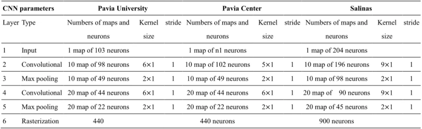
In this section, we apply the proposed method to three well known HSI data sets. We use different architectures of CNN for different HSI data sets. The CNN architectures of Pavia University, the CNN architectures of Pavia Center, and the architectures of Salinas are shown in Table 2. The architectures of CNN we used are very effective and our experiment results in three well known HSI data sets demonstrate the feasibility of the architecture.
Table 2 The architecture of CNN with Pavia University, Pavia Center, Salinas
A. Introduction to the Three Datasets
1) ROSIS Pavia University HSI:
The first HSI data set was collected in 2001 by the Reflective Optics System Imaging Spectrometer (ROSIS) optical sensor which provides 103 bands after removing 12 noisiest bands with a spectral range coverage
CNN parameters Pavia University Pavia Center Salinas
Layer Type Numbers of maps and neurons
Kernel size
stride Numbers of maps and neurons
Kernel size
stride Numbers of maps and neurons
Kernel size
stride
1 Input 1 map of 103 neurons 1 map of n1 neurons 1 map of 204 neurons
2 Convolutional 10 map of 98 neurons 6 1 1 10 map of 102 neurons 5 1 1 10 map of 196 neurons 9 1 1 3 Max pooling 10 map of 49 neurons 2 1 1 10 map of 49 neurons 2 1 1 10 map of 98 neurons 2 1 1 4 Convolutional 20 map of 44 neurons 6 1 1 20 map of 44 neurons 6 1 1 20 map of 90 neurons 9 1 1 5 Max pooling 20 map of 22 neurons 2 1 1 20 map of 22 neurons 2 1 1 20 map of 45 neurons 2 1 1
ranging from 0.43 to 0.86 um. The size of the image in pixels is 610 340 with very high spatial resolution of 1.3 m and 9 ground truth classes. The numbers of training samples is 3921 (about 9%) of all labeled data, and all the labeled data are used for testing. Table 3 shows the train samples and test samples in our experiments.
2) ROSIS Pavia Center HSI:
The second HSI data set was the other urban image collected in 2001 by the ROSIS sensors over the center of the Pavia city. The data set has 1096×715 pixels which each has 102 spectral bands after removing 13 noisy bands. There are also nine classes of images, and the numbers of training and test samples of each class of the HSI are shown in Table 3 in our experiments. There are about 7456 labeled samples used for training, which accounts for about 5 percent of the total sample. In order to compare the classification accuracy with other state-of-the-art methods, we use the rest labeled samples for testing.
3) AVIRIS Salinas HSI:
The third HSI data set was collected by the AVIRIS sensor over Salinas Valley, California. The image has 214 pixels and every pixels has 224 bands. After removing 20 water absorption bands of spectral, only 204 bands in each pixel. There are 16 classes in the ground truth image and the number of training and test are shown in Table 3. In order to facilitate classification accuracy comparison with other state-of-the-art method, we also use rest labeled samples for testing.
It is worth noting that in our experiments, the final output layer of the CNN architectures is only used during training. It facilitates the update of the weights and bias in the back propagation process, so that it can extract spectral feature of depth. We do not need to use the final output layer in the test process. We directly use the reconstructed spectral feature of the seventh layer as input of ELM. In order to maintain the high speed of the algorithm, we let CNN iteration only one time to reduce the time-consuming in the experiment. It is found that it can obtain high classification accuracy with little time-consuming. For the three HSI data sets, all the training
samples are randomly selected from each class in the labeled samples, and all experiment results of proposed method were averaged by ten times in Monte Carlo runs.
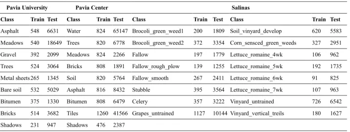
Table 3 The training sample and test sample of Pavia University, Pavia Center and Salinas.
Table 4 The hidden nodes of ELM after CNN reconstruct pixel of HSI.
B. The experiments results and analysis of Pavia University data set
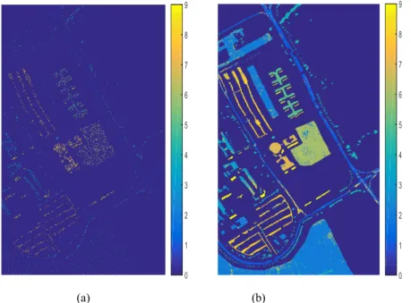
In this HSI data set of experiment, we evaluate the proposed method by comparing with other methods of state-of-the-art HIS using the University of Pavia data set. Fig. 4(a) and (b) show the training sample and the classification results with 3921 training samples and all the labeled samples, respectively. Table 5 shows the OA
(overall accuracy), AA (average accuracy), k (kappa coefficient) and individual class accuracies of the proposed method and other state-of-the-art methods. In contrast to other methods, our proposed method gets the best results with the same training samples (about 9% of available samples). Table 3 shows the training samples and test samples of Pavia University data set in this experiment.
Pavia University Pavia Center Salinas
Class Train Test Class Train Test Class Train Test Class Train Test
Asphalt 548 6631 Water 824 65147 Brocoli_green_weed1 200 1809 Soil_vinyard_develop 620 5583 Meadows 540 18649 Trees 820 6778 Brocoli_green_weed2 372 3354 Corn_sensced_green_weeds 327 2951 Gravel 392 2099 Meadows 824 2266 Fallow 197 1779 Lettuce_romaine_4wk 106 962 Trees 524 3064 Bricks 808 1891 Fallow_rough_plow 139 1255 Lettuce_romaine_5wk 192 1735 Metal sheets 265 1345 Soil 820 5764 Fallow_smooth 267 2411 Lettuce_romaine_6wk 91 825 Bare soil 532 5029 Asphalt 816 8432 Stubble 395 3564 Lettuce_romaine_7wk 107 963 Bitumen 375 1330 Bitumen 808 6479 Celery 357 3222 Vinyard_untrained 726 6542 Bricks 514 3682 Tiles 1260 41566 Grapes_untrained 1127 10144 Vinyard_vertical_treils 180 1627 Shadows 231 947 Shadows 476 2387
HSI data set The numbers of hidden nodes
Pavia University 900
Pavia Center 900
Salinas 1100
(a) (b)
Fig. 4. Pavia University data set: (a) Training samples; (b) Testing classification results.
Compared with ELM [32], our proposed method is superior to ELM for the classification accuracy of each class. In Table 5, we can see that for each class, we improve the classification accuracy all, and for the OA, AA, k, we improve 13.72%, 9.85%, 17.95%, respectively. It shows that our method improves the classification accuracy a lot.
Table 5 PAVIA University: Overall, Average, and individual class accuracy (in percent) and k statistic of different classification methods with 9% training samples. The best accuracy in each row is show bold.
Class [35] [32] CNN-ELM Asphalt 79.85 95.36 77.17 93.64 88.48 95.70 94.57 77.27 89.54 Meadows 84.68 63.72 81.61 97.35 76.22 73.27 82.56 77.53 94.14 Gravel 81.87 98.87 82.42 96.23 73.56 74.18 81.13 80.14 86.51 Trees 96.36 95.41 95.46 97.92 98.76 97.85 95.01 95.69 97.17 Metal sheets 99.37 87.61 99.03 66.12 99.70 99.85 100.0 99.69 98.94 Bare soil 93.55 80.33 96.94 75.09 97.47 98.55 100.0 80.47 94.02 Bitumen 90.21 99.48 93.83 99.91 94.74 97.97 99.17 82.97 95.17 Bricks 92.81 97.68 94.65 96.98 96.66 98.89 98.45 70.27 91.16 shadows 95.35 98.37 97.47 98.56 99.37 93.56 95.45 93.49 99.49 OA 87.18 85.22 86.16 85.42 85.69 85.78 90.01 79.58 93.30 AA 90.47 90.76 90.95 91.31 91.66 92.20 94.04 84.17 94.02 k 83.3 80.86 82.40 81.30 81.90 82.05 87.2 73.26 91.21 2 Meadows 3 Gravel 4 Trees 5 Metal sheets 6 Bare soil 7 Bitumen 8 Bricks 9 Shadows
Notes: The results of S‡M CK 襦For SVM, which use CK(composite kernel) that combines the spectral information and spatial information via a weighted kernel summation襤, LORS�L CK (For logistic regression via splitting and augmented Lagrangian, combine LORSAL with CK) LORS�L MLL (combine LORSAL with multilevel logistic spatial prior) and SMLR Sp�T‡ (combine sparse multinomial logistic regression with Markov random field) are directly taken from [33]. The results of EMP S‡M are directly taken from [34], which used EMPs for spectral-spatial characterization prior to SVM-based classification. The results of �atershed are directly taken from [35], which used a spectral-spatial classifier based on a pixel-wise SVM classifier with majority voting within the watershed regions to produce to final segmentation. The results of MPM L�P are directly taken from [36], a spectral-spatial method. The results of ELM are directly taken from [32]. CNN-ELM is the proposed method.
C. The experiments results and analysis of Pavia Center data set
In this experiment of HSI data sets, we evaluate the classification accuracy of the proposed method by comparing with other methods of state-of-the-art HSI classification. Fig.5 (a) and (b) show the training sample and the classification results of the proposed method with 7456 training samples and remaining samples, respectively. Table 6 shows the OA (overall accuracy), AA (average accuracy), k (kappa coefficient), and each
class’ accuracy. In contrast to other methods, the experiment results demonstrate our proposed method yields
the best results with the same training samples (about 5% of available samples) and test samples. The training samples and test samples of this experiment are shown in Table 3. The experiment results demonstrate our proposed method achieves higher accuracies than other method.
Compared with ELM [38] in Table 6, we can see that our proposed method not only improve classification accuracies of each class, but also improve the OA, AA, and k. For the OA, AA, and k, we improve 4.33%, 12.98%
(a) (b)
Fig. 5. Pavia Center data set: (a) Training samples; (b) Testing classification results.
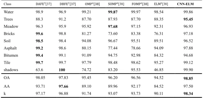
Table 6 PAVIA Center: Overall, Average, and individual class accuracy (in percent) and k statistic of different classification methods with 5% training samples. The best accuracy in each row is shown in bold.
Class D��E[37] D��E OMP SOMP[38] �OMP ELM[38] CNN-ELM
Water 98.9 96.9 99.21 99.87 99.97 98.54 99.86 Trees 88.3 91.2 87.70 87.93 87.70 88.35 95.45 Meadow 96.3 95.9 95.92 97.68 97.15 92.31 96.93 Bricks 99.6 98.8 81.27 73.60 83.38 76.31 97.18 Soil 98.5 98.4 94.08 96.67 95.51 89.51 96.52 Asphalt 99.2 98.6 80.15 77.44 78.66 94.09 97.88 Bitumen 99.4 99.1 91.09 94.75 92.98 84.32 94.68 Tile 99.7 99.7 97.79 98.48 98.62 95.27 99.12 shadows 63.6 100 74.72 83.20 95.53 46.85 99.90 OA 98.05 97.83 95.45 96.20 96.56 94.52 98.85 AA 93.71 97.66 89.10 89.96 92.17 84.52 97.50 k 97.17 96.88 91.74 93.07 93.73 90.11 98.34
Notes: The results of D��E (using the mean vector and the covariance matrix of each class for classification) and D��E (both discriminated informative features and redundant features can be extracted from the decision boundary between two classes) are directly taken from [37]. The result of OMP (Orthogonal Matching Pursuit), SOMP (Simultaneous Orthogonal Matching Pursuit), �OMP (First-order neighborhood system weighted constraint OMP), ELM are directly taken from [38]. CNN-ELM is the proposed method.
1Water 2Trees 3Meadow 4Bricks 5Soil 6Asphalt 7Bitumen 8Tile 9Shadows
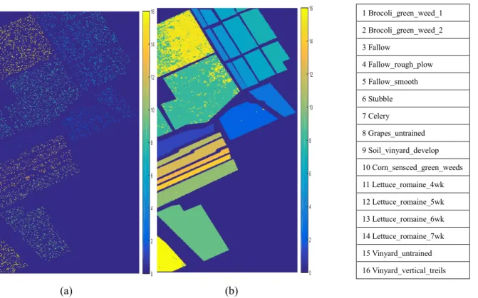
D. The experiments results and analysis of AVIRIS Salinas data set
(a) (b)
Fig. 6 Salinas data set: (a) Training samples; (b) Testing classification results.
In this HSI set of experiment, we evaluate our proposed method using the Salinas data sets. Table 7 shows the OA, AA and k statistic of our methods and the other methods using 10% training samples. Fig.6 (a) and (b) show the training sample and the classification results of the proposed method with 5403 training samples and remaining samples, respectively. Table 3 shows the numbers of training samples and the test samples of each class. It can be seen that our proposed method achieved better performance than other state-of-the-art HSI classification method.
From Table 7, we can see that the proposed method achieves better performance than ELM [38]. For the OA,
AA, k, the proposed method is higher than ELM with 6.22%, 4.98%, 6.94%, respectively.
Table 7. SALINAS:overall, average, and individual class accuracy (in percent) and k statistic of different classification methods with 10% training samples. The best accuracy in each row is shown in bold.
1 Brocoli_green_weed_1 2 Brocoli_green_weed_2 3 Fallow 4 Fallow_rough_plow 5 Fallow_smooth 6 Stubble 7 Celery 8 Grapes_untrained 9 Soil_vinyard_develop 10 Corn_sensced_green_weeds 11 Lettuce_romaine_4wk 12 Lettuce_romaine_5wk 13 Lettuce_romaine_6wk 14 Lettuce_romaine_7wk 15 Vinyard_untrained 16 Vinyard_vertical_treils
Class SR[39] KSR[39] S‡M[38] OMP[38] SOMP[38] ELM[38] CNN-ELM
Notes: The results of SR (Sparse Representation) and KSR (Kernel Sparse Representation) are directly taken from [39]. The results of S‡M , OMP , SOMP and ELM are directly taken from[38]. The CNN-ELM is the proposed method.
E. Impact of hidden neurons of ELM
In this experiment, we conduct an evaluation of the impact of the numbers of hidden neurons of ELM using Pavia University, Pavia Center and Salinas. The number of hidden neurons of ELM is an important parameter for HSI classification, so it is worthy to discuss.
Fig.7 (a), (b) and (c) plot the OA, AA, and kappa statistic results as a function of variable l (the numbers of hidden neurons of ELM) with 3921, 7456 and 5403 training samples, respectively. From Fig. 7(a), (b) and (c), we can see that l is an important parameter for HSI classification. It can be seen that, for Pavia University and Pavia Center data sets, we should choose 900 hidden neurons. But for the Salinas data sets, we should choose 1100 hidden neurons. By choosing appropriate hidden layer nodes, we obtain the best classification accuracy for ELM. For the training samples, we choose them randomly of each class in the all labeled samples.
Brocoli_green_weed_2 99.34 99.28 100 99.43 99.52 97.17 99.70 Fallow 97.58 97.47 98.99 96.68 97.81 91.57 99.78 Fallow_rough_plow 99.52 99.52 99.44 99.60 99.36 90.52 99.68 Fallow_smooth 98.26 98.18 99.17 97.06 96.43 93.28 98.80 Stubble 99.75 99.69 99.94 99.89 99.86 99.55 99.52 Celery 99.84 99.78 99.72 99.60 99.41 98.98 99.44 Grapes_untrained 87.67 89.73 89.79 78.77 82.29 81.66 89.51 Soil_vinyard_develop 99.73 99.70 99.80 99.12 99.44 96.96 99.87 Corn_sensced_green_weeds 96.81 96.75 95.29 95.39 94.71 86.00 97.19 Lettuce_romaine_4wk 98.23 98.02 97.51 97.71 96.88 93.14 99.69 Lettuce_romaine_5wk 100 99.88 99.60 99.65 100 99.37 100 Lettuce_romaine_6wk 99.15 98.91 97.45 97.58 96.00 96.73 97.70 Lettuce_romaine_7wk 96.37 96.16 93.67 94.91 96.57 92.00 97.20 Vinyard_untrained 67.85 67.82 67.84 65.81 71.29 60.29 78.43 Vinyard_vertical_treils 99.45 99.32 98.46 98.46 98.40 94.65 94.78 OA 92.48 92.42 92.83 89.99 91.46 87.91 94.13 AA 96.21 96.10 96.01 94.95 95.49 91.97 96.95 k 93.45 93.27 92.00 88.85 90.49 86.51 93.45
From Fig.7 (a) and Fig.8, we can see that the classification results are different with different l. The classification results of OA, AA, kappa statistic of Pavia University is 93.30%, 94.02%, 91.21%, respectively when the hidden neurons of ELM is set to 900, and the classification results with 900 hidden neurons of ELM outperforms other classification results with 300, 600, 1200 and 1500 hidden neurons.
From Fig.7 (b) and Fig (9), although the AA of 1200 and 1500 hidden neurons are higher than 900 hidden neurons, the 900 hidden neurons achieve the best OA and kappa statistic. The OA, AA, kappa statistic with 900 hidden neurons is 98.85%, 97.50% and 98.34%, respectively. So we can say that 900 hidden neurons are the best choice for Pavia data sets.
The same as Pavia Center, from Fig 7 (c) and Fig 10, we can know that the AA is higher with 1400 hidden neurons than AA with 1100 hidden neurons, but the 1100 hidden neurons achieve the best classification results. So 1100 hidden neurons are the best choice for Salinas data sets.
(a) (b) (c) Fig. 7. The impact of hidden neurons of ELM: (a) Pavia University; (b) Pavia Center; (c) Salinas.
(a) (b) (c) (d) (e)
Fig.8. The different classification results of Pavia University: (a) 300 hidden neurons of ELM with 91.27% (OA); (b) 600 hidden neurons of ELM with 93.16% (OA); (c) 900 hidden neurons of ELM with 93.3% (OA); (d) 1200 hidden neurons of ELM with 93.18% (OA); (e) 1500 hidden neurons of ELM with 92.49% (OA).
(a) (b) (c)
(d) (e)
Fig.9. The different classification results of Pavia Center: (a) 300 hidden neurons of ELM with 98.57% (OA); (b) 600 hidden neurons of ELM with 98.75% (OA); (c) 900 hidden neurons of ELM with 98.85% (OA); (d) 1200 hidden neurons of ELM with 98.77% (OA); (e) 1500 hidden neurons of ELM with 98.68% (OA).
(a) (b) (c)
(d) €
(d) (e)
Fig.10. The different classification results of Salinas: (a) 500 hidden neurons of ELM with 93.84% (OA); (b) 800 hidden neurons of ELM with 94.08% (OA); (c) 1100 hidden neurons of ELM with 94.15% (OA); (d) 1400 hidden neurons of ELM with 94.14% (OA); (e) 1700 hidden neurons of ELM with 94.00% (OA).
V Conclusions
In this paper, we have proposed a new method for HSI classification by combining CNN with ELM, where spectral features reconstructed by using CNN was used as input to ELM for classification. Experiment results on three HSI data sets have demonstrated that the reconstructed spectral greatly improves the classification accuracy of HSI data sets, where it is shown that the hidden neurons of ELM is essential for improved HSI classification. In general, the proposed approach has achieved the best results among several state-of-the-art approaches.
is also important for HSI classification, so the future work will focus on using the spatial information for improve the accuracy.
Acknowledgements
The work is partially supported by the University of Strathclyde and the following grants: National Natural
Science Foundation of China (61272381, 61471132, 61401163), Science and Technology Major Project of Education
Department of Guangdong Province (2014KZDXM060), the Fundamental Research Funds for the Central
Universities (No.2015ZZ032), and Science and Technology Project of Guangzhou City (2014J4100078).
References
[1] A. Wang, J. Lu, J. Cai , et al, “Unsupervised joint feature learning and encoding for rgb-d scene labeling,” IEEE Transactions on Image Processing, vol.24, no.11, pp.4459-4473, 2015.
[2] S. Yu, S. Jia, C. Xu, “Convolutional neural networks for hyperspectral image classification,” Neurocomputing, vol. 219, pp. 88-98, 2017. [3] M. Sun, D. Zhang, Z. Wang, J. Ren, and J. S. Jin, “Monte Carlo convex hull model for classification of traditional Chinese paintings,”
Neurocomputing, vol. 171, pp. 788-797, 2016.
[4] F. Melgani, L. Bruzzone, “Classification of hyperspectral remote sensing images with support vector machines,” IEEE Transactions on
geoscience and remote sensing, vol. 42, no. 8, pp. 1778-1790, 2004.
[5] T. Qiao, J. Ren et al, “Effective denoising and classification of hyperspectral images using curvelet transform and singular spectrum analysis,” IEEE Trans. Geoscience and Remote Sensing, vol. 55, no. 1, pp. 119-133, 2017.
[6] J. Zabalza, J. Ren, J. Zheng, J. Han, H. Zhao, S. Li, and S. Marshall, “Novel two dimensional singular spectrum analysis for effective feature extraction and data classification in hyperspectral imaging,” IEEE Trans. Geoscience and Remote Sensing, vol. 53, no. 8, pp. 4418-4433, 2015. [7] T. Qiao, J. Ren, C. Craigie, Z. Zabalza, C. Maltin, S. Marshall, “Singular spectrum analysis for improving hyperspectral imaging based beef
eating quality evaluation,” Computers and Electronics in Agriculture, 2015.
[8] X. Lu, Y. Wang, Y. Yuan, “Graph-Regularized Low-Rank Representation for Destriping of Hyperspectral Images,” IEEE Trans. Geoscience and Remote Sensing, vol. 51, pp. 4009-4018, 2013.
[9] Y. Yuan, X. Zheng, X. Lu, “Discovering Diverse Subset for Unsupervised Hyperspectral Band Selection,” IEEE Trans. Image Processing, vol. 26, no. 1, pp. 813-822, 2017.
[10] J. Zabalza, J. Ren, M. Yang, Y. Zhang, J. Wang, S. Marshall, J. Han, "Novel Folded-PCA for Improved Feature Extraction and Data Reduction with Hyperspectral Imaging and SAR in Remote Sensing," ISPRS Journal of Photogrammetry and Remote Sensing, vol. 93, no. 7, pp. 112-122, 2014.
[11] L. Fang, S. Li, W. Duan, J. Ren, J. Atli Benediktsson, "Classification of hyperspectral images by exploiting spectral-spatial information of superpixel via multiple kernels," IEEE Trans. Geoscience and Remote Sensing, vol. 53, no. 12, pp. 6663-6674, 2015.
[12] J. Zabalza, J. Ren, J. Zheng, H. Zhao, C. Qing, Z. Yang, P. Du and S. Marshall, “Novel segmented stacked autoencoder for effective
dimensionality reduction and feature extraction in hyperspectral imaging,” Neurocomputing, vol. 185, pp. 1-10, 2016
[13] Z. Du, X. Li, X. Lu, “Local structure learning in high resolution remote sensing image retrieval,” Neurocomputing, vol. 207, pp. 813-822, 2016.
on Geoscience and Remote Sensing, vol. 48, no. 11, pp. 4099-4109, 2010.
[15] J. Li, J. M. Bioucas-Dias, A. Plaza, “Spectral–spatial hyperspectral image segmentation using subspace multinomial logistic regression and Markov random fields,” IEEE Transactions on Geoscience and Remote Sensing, vol. 50, no. 3, pp.809-823, 2012.
[16] J. Li, J. M. Bioucas-Dias, A. Plaza, “Semisupervised hyperspectral image segmentation using multinomial logistic regression with active
learning,” IEEE Transactions on Geoscience and Remote Sensing, vol. 48, no. 11, pp. 4085-4098, 2010
[17] G. B. Huang, Q. Y. Zhu, C. K. Siew, “Extreme learning machine: a new learning scheme of feedforward neural networks,” Neural Networks, Proceedings. 2004 IEEE International Joint Conference on. IEEE, pp. 2: 985-990, 2004.
[18] Z. Bai, G. B. Huang, D. Wang, et al, “Sparse extreme learning machine for classification. IEEE transactions on cybernetics,” vol. 44, no. 10,
pp. 1858-1870, 2014.
[19] G. B. Huang, H. Zhou , X. Ding , et al, “Extreme learning machine for regression and multiclass classification,” IEEE Transactions on Systems, Man, and Cybernetics, Part B (Cybernetics), vol. 42, no. 2, pp. 513-529, 2012
[20] A. Samat , P. Du , S. Liu, et al, “Ensemble Extreme Learning Machines for Hyperspectral Image Classification,” IEEE Journal of Selected
Topics in Applied Earth Observations and Remote Sensing, vol. 7, no. 4, pp. 1060-1069, 2014
[21] G. E. Hinton, R. R. Salakhutdinov, “Reducing the dimensionality of data with neural networks,” Science, vol. 313, no. 5786, pp. 504-507, 2006
[22] W. Hu, Y. Huang, L. Wei, et al, “Deep convolutional neural networks for hyperspectral image classification,” Journal of Sensors, 2015.
[23] K. Fukushima, Neocognitron, “A hierarchical neural network capable of visual pattern recognition,” Neural networks, vol. 1, no. 2, pp.
119-130, 1988.
[24] Y. LeCun , L. Bottou, Y. Bengio, et al, “Gradient-based learning applied to document recognition,” Proceedings of the IEEE, vol. 86, no. 11, pp. 2278-2324,1998.
[25] D. C. Ciresan, U. Meier, J. Masci, et al, “Flexible, high performance convolutional neural networks for image classification,” IJCAI Proceedings-International Joint Conference on Artificial Intelligence, vol. 22, no. 1, pp. 1237,2011
[26] P. Y.Simard, D. Steinkraus, J. C. Platt, “Best practices for convolutional neural networks applied to visual document analysis,” ICDAR, vol. 3, pp. 958-962, 2003.
[27] V. Slavkovikj, S. Verstockt, W. De Neve, et al, “Hyperspectral image classification with convolutional neural networks,” Proceedings of the 23rd ACM international conference on Multimedia. ACM, pp. 1159-1162, 2015.
[28] J. Yue, W. Zhao, S. Mao, et al, “Spectral–spatial classification of hyperspectral images using deep convolutional neural networks,” Remote Sensing Letters, vol. 6, no. 6, pp. 468-477, 2015.
[29] K. Makantasis, K. Karantzalos, A. Doulamis, et al, “Deep supervised learning for hyperspectral data classification through convolutional neural networks,” 2015 IEEE International Geoscience and Remote Sensing Symposium (IGARSS). IEEE, pp. 4959-4962, 2015.
[30] G. B. Huang, D. H. Wang, Y. Lan, “Extreme learning machines: a survey,” International Journal of Machine Learning and Cybernetics, vol. 2, no. 2, pp. 107-122, 2011.
[31] T. N. Sainath, A. Mohamed, B. Kingsbury, et al, “Deep convolutional neural networks for LVCSR,” 2013 IEEE International Conference on Acoustics, Speech and Signal Processing. IEEE, pp.8614-8618, 2013.
[32] Q. Lv, X. Niu, Y. Dou, et al, “Classification of hyperspectral remote sensing image using hierarchical local-receptive-field-based extreme
learning machine,” IEEE Geoscience and Remote Sensing Letters, vol. 13, no. 3, pp. 434-438, 2016.
[33] L. Sun, Z. Wu, J. Liu, et al, “Supervised spectral–spatial hyperspectral image classification with weighted Markov random fields,” IEEE Transactions on Geoscience and Remote Sensing, vol. 53, no. 3, pp. 1490-1503, 2015.
[34] A. Plaza, J. A. Benediktsson, J. W. Boardman, et al, “Recent advances in techniques for hyperspectral image processing,” Remote sensing of
environment, vol. 113, pp. 110-122, 2009.
[35] Y. Tarabalka, J. Chanussot, J. A. Benediktsson, “Segmentation and classification of hyperspectral images using watershedtransformation,”
Pattern Recognition, vol. 43, no. 7, pp. 2367-2379, 2010.
[36] J. Li, J. M. Bioucas-Dias, A. Plaza, “Spectral–spatial classification of hyperspectral data using loopy belief propagation and active learning,” IEEE Transactions on Geoscience and Remote Sensing, vol. 51, no. 2, pp. 844-856, 2013.
[37] P. Ghamisi, J. A. Benediktsson, J. R. Sveinsson, “Automatic spectral–spatial classification framework based on attribute profiles and
supervised feature extraction,” IEEE Transactions on Geoscience and Remote Sensing, vol. 52, no. 9, pp. 5771-5782, 2014.
[38] Y. Li, W. Xie, H. Li, “Hyperspectral image reconstruction by deep convolutional neural network for classification,” Pattern Recognition, vol. 63,pp. 371-383, 2017.
[39] X. Zhang, Y. Liang, Y. Zheng, et al, “Hierarchical Discriminative Feature Learning for Hyperspectral Image Classification,” IEEE