Unequal Probability Sampling in Active Learning and Traffic Safety

T

D

L

P

Unequal Probability Sampling in

Active Learning and Traffic Safety

HENRIK

I

MBERG

Division of Applied Mathematics and Statistics Department of Mathematical Sciences

Chalmers University of Technology and University of Gothenburg Gothenburg, Sweden 2019

c

Henrik Imberg, 2019

Division of Applied Mathematics and Statistics Department of Mathematical Sciences

Chalmers University of Technology and University of Gothenburg SE-412 96 Gothenburg, Sweden

Telephone +46 (0)31 772 10 00

Author e-mail:[email protected]

Typeset with LA_TEX

Printed by Chalmers Digitaltryck Gothenburg, Sweden 2019

Unequal Probability Sampling in Active Learning

and Traffic Safety

Henrik Imberg

Division of Applied Mathematics and Statistics Department of Mathematical Sciences

Chalmers University of Technology and University of Gothenburg

Abstract

This thesis addresses a problem arising in large and expensive experiments where incomplete data come in abundance but statistical analyses require collection of additional information, which is costly. Out of practical and economical considerations, it is necessary to restrict the analysis to a subset of the original database, which inevitably will cause a loss of valuable information; thus, choosing this subset in a manner that captures as much of the available information as possible is essential.

Using finite population sampling methodology, we address the issue of appro-priate subset selection. We show how sample selection may be optimised to maximise precision in estimating various parameters and quantities of interest, and extend the existing finite population sampling methodology to an adap-tive, sequential sampling framework, where information required for sample scheme optimisation may be updated iteratively as more data is collected. The implications of model misspecification are discussed, and the robustness of the finite population sampling methodology against model misspecification is highlighted.

The proposed methods are illustrated and evaluated on two problems: on subset selection for optimal prediction in active learning (Paper I), and on optimal control sampling for analysis of safety critical events in naturalistic driving studies (Paper II). It is demonstrated that the use of optimised sample selection may reduce the number of records for which complete information needs to be collected by as much as 50%, compared to conventional methods and uniform random sampling.

Keywords: active learning; naturalistic driving; optimal design; probability sampling; sampling weighing; sequential sampling.

List of publications

This thesis is based on the work represented in the following manuscripts:

I. Imberg, H., Jonasson, J., Axelson-Fisk, M. (2019). Optimal sampling in unbiased active learning.Submitted.

II. Imberg, H., Lisovskaja, V., Selpi, Nerman, O. (2019). Optimisation of two-phase sampling designs with application to naturalistic driving studies.Submitted.

Author contributions

I. Derived and proved the theoretical results, developed and wrote the implementation of the method, performed data analysis, drafted and edited the manuscript.

II. Developed and wrote the implementation of the method, performed data analysis, drafted and edited the manuscript.

Acknowledgements

First and foremost I would like to thank my supervisor Marina Axelson-Fisk, for your continuous support and engagement, and Johan Jonasson, for always highlighting the importance of mathematical rigour. Thanks to Olle Nerman for your thoughtful comments and our many discussions, for the insights these have given me. Thanks to Selpi and Vera Lisovskaja for carefully reading my manuscripts. Thanks also to Per-Gösta Andersson for teaching me asymptotics, to Martin Raum for letting me run my computations on your high performance computing machine Gantenbein, and to Rune Imberg for punctilious proofreading.

I would also like to thank all my colleagues and fellow PhD students at the Department of Mathematical Sciences. Thanks especially to Helga Kristin Olafsdottir, Olle Elias, Ed-vin Wedin, Linnea Hietala, Anna Rehammar, Malin Palö Forsström, Johannes Borgqvist, Oskar Allerbo, and Felix Held; I always enjoy your company. Thanks also to anyone I may have forgotten to mention.

Finally, I would like to thank my wife, Ida, for all your love and support, and my children, Hilma and Aron, for all the joy you bring and for pinpointing what’s important in life.

Contents

2 Background: Sampling from a finite universe 5 3 Methodological considerations and contributions 11 3.1 Optimal sampling schemes . . . 11 3.2 Sequential subsampling . . . 16 3.3 Robustness against model misspecification . . . 19

4 Summary of papers 25 4.1 Paper I . . . 25 4.2 Paper II . . . 28 Bibliography 31 Papers I and II ix

1 Introduction

With the advances of modern technology, data are currently being generated at greater volume than ever before. The impact of this progression can hardly pass unnoticed in our private and social lives, and may be recognised in nearly all fields of scientific research. Indeed, these new data sources do, by application of appropriate scientific methods, offer opportunities to gain insights and knowledge in a way that previously could not be imagined. Yet, the complexity of many of these new data sources and the sheer amount of data being collected introduces new challenges of statistical data analysis, requiring development of new statistical methods and adaptation of existing methods to novel problem settings.

A common theme for the papers included in this thesis is the application of statistical methods from the field of survey sampling, much of which was developed many decades ago, to modern problems within the fields of ma-chine learning and traffic safety research. The survey sampling methodology was initially developed for the purpose of performing descriptive analyses of finite populations where complete enumeration was infeasible, e.g. for produc-ing national official statistics regardproduc-ing population, labour market, business etc. As will be demonstrated in this thesis, the finite population sampling methodology offers a promising approach for the analysis of large and complex databases also in modern problems where data reduction through subsampling is inevitable.

The specific problem we consider arises from large and expensive experiments with mixed data sources, where some measurements are cheap and easy to obtain for a very large number of subjects or instances, while others are ex-pensive to measure and thus are observable only for a small subset of a large population or database. This problem may be encountered in a wide range of applications, including medical studies, where medical screening may be affordable for a large number of subjects but intervention may be feasible only for a smaller number; bioinformatics, where modern sequencing techniques

enable collection of large scale genomic data at relatively low cost, but where in depth analysis may require expensive laboratory experiments; naturalistic driving studies, where vehicle data is recorded continuously for all driving sessions in a large fleet of vehicles, but the analysis requires manual annotation of video sequences; and machine learning problems such as image recognition and classification, where some variables stored in a database may be collected at large volumes and low cost, e.g. matrix representations of digital images, while others may require human annotation prior to analysis, e.g. what those images actually depict.

To put the stated problem into context, we consider in Paper II a naturalistic driving study, where data is collected automatically for all driving sessions in a large fleet of vehicles. These automatic recordings include, among oth-ers, vehicle data such as speed and direction; environmental conditions, lane position, location and surrounding traffic recorded by radar, video and other external instrumentation; and video recordings of driver’s face, pedal, and eye movements. From these data, we are interested in the impact of various driver and driving characteristics on the risk of a safety critical event such as a rear-end collision. Typically, some of the explanatory variables and/or the response variable require annotation of video sequences before statistical analysis can be conducted, which often is affordable only for a fraction of the driving sessions in the database. However, auxiliary information in terms of automatic recordings of vehicle manoeuvres etc. is readily available for all instances in the database. Using such information, it is possible to optimise the selection of which instances to annotate with regards to detection of potential associations between driving behaviour and a consecutive safety critical event. Another example, further considered in Paper I, is found in the field of ac-tive learning; an algorithmic framework where a semi-supervised learning algorithm iterates between data collection and model fitting by repeatedly querying the label of new instances from a large pool or stream of unlabelled observations, in order to derive a prediction model for an outcome of interest. In active learning problems, the variables used as predictors are known for all instances in a large database, but the outcomes require annotation or other means of manual investigation, which is costly, and are thus observable for a limited number of instances only. Again, this offers an opportunity to use available data in order to optimise sample selection, in this case to minimise prediction error.

Using finite population sampling methodology, we address the issue of ap-propriate subset selection from large databases where collection of complete information is unfeasible and subsampling is inevitable. We show how sam-ple selection may be optimised to maximise precision in estimating various

3

parameters and quantities of interest, by making use of information readily available for all records in the database, without compromising the validity of the statistical analysis and conclusions drawn from the collected sample.

2 Background: Sampling from

a finite universe

Consider a finite index setDconsisting ofNelementsi= 1, . . . , N. Associated with each element is a data vector(xi, yi,zi)that characterises each member

i ∈ D. We may think ofDas a database, where a collection of N records (xi, yi,zi)are stored or indirectly made accessible. In the terms of survey sampling, the index setDis commonly referred to as a finite population or a finite universe (Särndal et al., 2003).

The variablesX,Y andZstored in the databaseDare distinguished by their role in the statistical analyses, whereXare explanatory variables, covariates or predictors,Y is an outcome or response variable, andZare additional auxiliary variables that are co-stored in the database but not necessarily of interest in the statistical analyses. It is assumed that some variablesV, including the auxiliary variablesZand possibly also some components of(X, Y), are readily observed for all records in the database. However, some components of(X, Y), which we denote byU, require additional effort, associated with a high cost, to be fully observed. Thus, the variablesUmay be observed only for a subsetS ⊂ D. We are interested in estimating a parameterθ of a statistical modelfθ(y|x), describing the dependency of the outcomeY on the covariatesX, with the purpose of either describing the relationship between these variables or ob-taining a predictive modelf_θˆ(y|x)for the records in the current database or for future observations. In addition, we assume the existence of an auxiliary modelgη(u|v), describing the distribution of the unobserved variablesUgiven

the observed variablesV, which may be utilised for sample selection. The use of the auxiliary model for sample selection will be discussed in Chapter 3.1.2, and the modelgη(u|v)will not be considered further in this section.

For the purpose of estimating the parameterθof the modelfθ(y|x), we con-sider a twice-differentiable loss function`(y,x,θ), describing the loss

ated with the prediction derived from the pair(x,θ)when the true outcome is

y, and denote by`i(θ) =`(yi,xi,θ)the loss associated with an instancei∈ D for a specific parameter valueθ. Also, we let

`0(θ) = X

i∈D

`i(θ) (2.1)

denote the population loss as a function ofθ, and letθ0denote the correspond-ing optimal parameter in the sense that

θ0= arg min

θ

`0(θ) . (2.2)

As described above, we assume that some components of(X, Y)are expensive or difficult to measure and may be observed only for a subsetS ⊂ D. Con-sequently,`0(θ)andθ0can not be computed and subsampling is inevitable. We consider the situation where this subset is selected according to a random mechanism where each instancei ∈ D has a strictly positive probability of being sampled, denoted as probability sampling (Särndal et al., 2003). We introduce the random variableQias the number of times an instanceiis se-lected, assuming that sampling may be with replacement, and letνi:= E[Qi] denote the corresponding mean. Thus, the sampling mechanism is fully charac-terised by the multivariate distribution ofQ:= (Q1, . . . , QN). As an example, we may consider sampling according to independent Bernoulli(πi) trials, a process known as Poisson sampling (Särndal et al., 2003). In this case, the

Qi’s are binary random variables with meansνi =πi, and the subsampleS consists of all instances havingQi = 1; this is a random set with expected sizen:= E[|S|] = E[P

i∈DQi] =Pi∈Dπi. Sampling may alternatively be con-ducted according to a Multinomial(n, π1, . . . , πN) distribution, having sizen, meansνi=nπiand non-zero covariancesCov(Qi, Qj) =−nπiπj. Thus, Pois-son sampling and Multinomial sampling are both examples of unequal proba-bility sampling designs, the former being a random-size without-replacement design, and the latter a fixed-size with-replacement design. See e.g. Särndal et al. (2003) and Tillé (2006) for additional details on these and other probability sampling designs.

Consider now a specific probability sampleS ⊂ D, and suppose that complete records(xi, yi)have been observed for the elementsi ∈ S of the selected sample. Since different elements can have different sampling probabilities, ordinary maximum likelihood estimation or empirical risk minimisation, which assumes an i.i.d sample, is generally not applicable. Instead, we consider a

7

sampling-weighted estimatorθˆπ, defined as ˆ θπ:= arg min θ ˆ `π(θ) , (2.3) ˆ `π(θ) := X i∈S wi`i(θ) , (2.4)

where the sampling weightswimay be taken aswi=Qi/νi. With this choice of weights, the sum (2.4) is known as a Horvitz-Thompson estimator (Horvitz and Thompson, 1952) of the population loss`0(θ)if sampling is without re-placement, and as a Hansen-Hurwitz estimator (Hansen and Hurwitz, 1943) for sampling with replacement. In either case, it follows thatE[wi] = E[Qi]/νi = 1, and hence that`ˆπ(θ)is an unbiased estimator of the population loss`0(θ). Under general regularity conditions, including conditions on the statistical model and parameter space that enable Taylor expansions around the op-timal parameter, and additionally some conditions on the sampling design that govern the asymptotic properties of the Horvitz-Thompson or Hansen-Hurwitz estimator, it holds thatθˆπis asymptotically normal and consistent as an estimator ofθ0, with asymptotic covariance matrix

Varθˆπ−θ0 =H(θ0)−1Varπ ∇θ`ˆπ(θ0) H(θ0)−1+o(n−1) , (2.5) wherenis the size of the subsample S, H(θ)is the Hessian matrix of the population loss`0(θ), andVarπ(∇θ`ˆπ(θ0)denotes the covariance matrix, with respect to the sample selection mechanism, of the gradient of the weighted loss ˆ

`π(θ), evaluated atθ=θ0. Explicitly, we can write

Varπ ∇θ`ˆπ(θ0) =X i∈D Var(Qi) ν2 i sisTi + X i,j∈D i6=j Cov(Qi, Qj) νiνj sisTj , (2.6)

wheresi =si(yi,xi,θ0) :=∇θ`i(θ0)is the gradient of the loss pertaining to instanceievaluated atθ=θ0; see Binder (1983).

An important special case in the statistical literature arises when we take`(θ) as the logarithmic loss, i.e. take`(y,x,θ) =−logfθ(y|x). In this, case,`0(θ)is the negative of the log-likelihood based on the entire databaseD,θ0is the max-imum likelihood estimator ofθfrom the databaseD,−H(θ0)is the observed Fisher information matrix pertaining to the databaseD. The estimator ˆθπ, defined by (2.3) and (2.4), is in this setting also known as a weighted maximum likelihood estimator or pseudo maximum likelihood estimator (Skinner, 1989). The inferential framework outlined above is commonly referred to as design-based (Särndal et al., 2003), as opposed to the model-design-based inference proce-dures otherwise commonly employed. While in both cases we may consider

a statistical modelfθ(y|x), the two paradigms differ in their view on the ran-dom processes involved, and consequently on the assumptions needed for the corresponding inferences to be valid. From a model-based perspective, we think of the unknown responses as random variables{Yi}i∈D, following some unknown probability distribution. Consequently, the statistical prop-erties of estimators derived from model-based procedures are induced from the assumptions made by the modelfθ(y|x), and the validity of such infer-ence hinge on the correctness of these assumptions. From a design-based perspective, on the other hand, all randomness is ascribed to the sample selec-tion mechanism, and the outcomes{yi}i∈D are treated as fixed but possibly unknown constants; variation simply arises by random sampling from the databaseD. Consequently, the statistical properties of estimators derived from design-based procedures are induced by the sampling design, which is under direct control of the investigator, and is, with respect to inference regarding the finite population parameterθ0, free of modelling assumptions. Thus, the design-based approach possesses a desirable property in terms of robustness against model misspecification; see e.g. Pfeffermann (1993) and the discussion in Chapter 3.3.

While the model-based and design-based paradigms may seem incompatible given the discussion above, the two approaches to inference may in fact be combined; this is particularly useful in applications that require subsampling, but where interest is of analytic rather than descriptive nature, i.e. when one is interested in the underlying data generating mechanism rather than in the finite population parameterθ0. This is sometimes referred to as a ’super-population viewpoint’ for finite population sampling (Hartley and Sielken, 1975), where the super-population represents a hypothetical infinite population from which the databaseDis assumed to have been drawn. We can also recognise this as a two phase sampling procedure, where the databaseDis generated and some variables are observed in an initial phase, and a subset is selected for which complete data is collected in the second phase. Considering the joint model-and design-based inference regarding the true parameterθ∗, it holds under regular conditions that govern the convergence of model-based estimators in the law of the model and the convergence of design-based estimators in the law of the sampling design, that the estimatorˆθπis asymptotically normal and consistent as an estimator of the true parameterθ∗, with asymptotic covariance matrix

Var(ˆθπ−θ∗) = Var(θ0) + ED[Var(ˆθπ−θ0|D)] +o(n−1) ,

whereVar(θ0)is the variance ofθ0 =θ0(D)as an estimator ofθ∗using the complete dataD, andED[·]denotes the expectation with respect to the data generating mechanism, i.e. over all the potential datasetsD(Rubin-Bleuer and Schiopu Kratina, 2005; Fuller, 2009, Chapter 6.5). Thus, the first term accounts

9

for between-database variation, while the second term accounts for additional variation due to subsequent subsampling fromD. In the papers included in this thesis, the design-based perspective is dominant in Paper I, while in Paper II we consider a two-phase sampling scenario where our interest is to understand the underlying data generating mechanism.

3 Methodological considerations

and contributions

In this chapter, we present the contributions of our work and the solution we propose to the problem of subset selection from large databases for which complete data is affordable only for a limited subset. First, we derive optimal sampling schemes for a general class of optimality criteria, and show how these may be implemented by use of available auxiliary information. We then present an extension of the sampling methodology described in the previous chapter to a sequential subsampling framework, where the information re-quired for sample scheme optimisation may be updated iteratively as more data is collected. The chapter is concluded by a discussion on the implications of model misspecification, i.e. when there is a mismatch between the data generating mechanism and the analytic model on which inference is based, on statistical modelling in general and on the proposed inferential framework in particular.

3.1

Optimal sampling schemes

Considering the variance formulas (2.5) and (2.6) of the weighted estimatorˆθπ, we note that the variance depends on the sampling design in a rather simple manner, apart from potential complications from the covariancesCov(Qi, Qj). Thus, for certain sampling designs, it is possible to formulate optimality criteria in terms of the variances of linear combinations of the model parameterθas convex optimisation problems for which explicit solutions may be obtained. In the terminology of optimal design theory, this class of optimality criteria is referred to as L-optimality, and includes, as a special case, optimisation with respect to the average variance of an estimator of a parameter vector, known

as A-optimality (Atkinson and Donev, 1992). Using linearisation techniques, the results may be extended also to smooth non-linear functions ofθ, enabling optimisation with respect to a wide range of commonly used statistics. In what follows, we restrict the presentation to sampling according to inde-pendent Bernoulli(πi) trials, i.e. Poisson sampling, or according to a Multi-nomial(n,π) distribution, takingπ as the vector (π1, . . . , πN). We let ||v|| denote the Euclidean norm of a vectorv, i.e. ||v||=√vT_{v, and consider, to} begin with, a linear combinationaTθ =a1θ1+a2θ2+. . . apθpof the model parametersθ = (θ1, . . . , θp), wherea is a vector of linear coefficients. For instance, in the context of regression modelling, such a linear combination may describe the effect of a single covariate on the outcomeY, or the effect associated with a simultaneous change in multiple covariates.

Using Poisson sampling, the asymptotic variance of the sampling-weighted estimatoraT_θˆ

πof such a linear combination is given by

Var(aTθˆπ−aTθ0) =aTH(θ0)−1 X i∈D 1−πi πi sisTi ! H(θ0)−1a+o(n−1) ,

following from the fact thatVar(Qi) =πi(1−πi)andCov(Qi, Qj) = 0. Simi-larly, the variance ofaT_θˆ_{πunder multinomial sampling is given by}

Var(aT_kˆθπ−aTkθ0) = aTH(θ0)−1 1 n    X i∈D 1−πi πi sisTi − X i,j∈D i6=j πiπj πiπj sisTj   H(θ0) −1_a+o(n−1_{) ,}

following from the fact thatνi := E[Qi] = nπi,Var(Qi) = nπi(1−πi)and Cov(Qi, Qj) =−nπiπj. In either case, we note that the variance can be written as Var(aT_kθˆπ−aTkθ0) = X i∈D ci πi +k+o(n−1) , where ci=c(θ0) =||aTH(θ0)−1si||2 (3.1) andkis a constant not depending onπ. It follows that the optimal sampling scheme in terms of minimising this variance is obtained by choosing

πi∝ √

ci , (3.2)

which in the case of Poisson sampling should be normalised so thatP i∈Dπi equals the desired sample size, and for Multinomial sampling so thatP

3.1. Optimal sampling schemes 13

1. For Poisson sampling, however, this may result in sampling probabilities greater than one, a situation that is handled in Algorithm 1 in Appendix A of Paper II. For a proof of the optimality of these sampling schemes, we refer to Appendix B of Paper II.

More generally, consider a collection of parameter combinations captured by an (rxp) matrixL, where each rowaT_k ofLdefines a linear combination as described above. Thus, the matrixLmay be defined to capture several relevant evaluations and comparisons of interest. Using the sum of variances of the linear combinations specified by the matrixLas optimality criterion, the result in Equation (3.1) and (3.2) generalises to

ci=||LH(θ0)−1si||2 . (3.3)

In the survey sampling literature, it is a well known fact that optimal preci-sion of the Hansen-Hurwitz and Horvitz-Thompson estimators of a simple population characteristic, such as a total or mean, is achieved by assigning probabilities proportional to the size of the characteristic of interest, denoted as PPS sampling (Hansen and Hurwitz, 1943; Horvitz and Thompson, 1952; Särn-dal et al., 2003). Similarly, we may interpret the sampling design obtained from takingπiaccording to (3.2) as a PPS sampling design, where ’size’ is measured in terms of the influence on estimating the linear combinations{aT

kθ}rk=1, as measured by||LH(θ0)−1si||.

The proposed sampling strategy also has some interesting connections to leverage sampling (Ma et al., 2014; Ma and Sun, 2015; Ma et al., 2015) and robust inference (Huber and Ronchetti, 2009), the former being based on the the idea that influential data points should be oversampled, as these anyway would drive most of the fit, and the latter being based on the idea that influential data points should be down-weighted to reduce variance. By use of PPS sampling and inverse probability weighing, variance reduction is achieved by simultaneous oversampling and down-weighing of influential data points.

3.1.1

Non-linear optimality criteria

Using linearisation techniques, we can apply the same procedure as above to optimisation with respect to non-linear optimality criteria, provided that these can be expressed in terms of smooth functions of the parameterθ. Specifically, consider a differentiable functionh:_R→Rwith derivativeh0. Using the the

Delta method (DasGupta, 2008), the asymptotic variance ofh(aT_θˆ

expressed in terms of the variance ofθˆπas

Varh(aTˆθπ)−h(aTθ0)

=aTh0(aTθ0)Var(ˆθπ−θ0)h0(aTθ0)a+o(n−1) , provided that the first term of the right hand side is greater than zero. Hence, minimising the average variance ofh(aT

1θˆπ),. . .,h(aTrθˆπ)translates into a linear optimality criterion, takingLas the matrix with rowsh0(aT

kθ0)aTk. We note that many commonly used statistics may be described in terms of smooth non-linear functions of the parameterθand thus fit into the presented framework, including e.g. the coefficient of determination for linear regression models, and estimates of odds ratios, absolute risks and relative risks in binary logistic regression.

As another example, further considered in Paper I, the use of linearisation techniques enables sample scheme optimisation with respect to prediction vari-ance from a wide range of parametric statistical models. Specifically, suppose that the expectation ofY, under the modelfθ(y|x), can be expressed in terms of a twice differentiable functionµ : R → RasEθ[Y|x] = µ(xTθ). This is

commonly the case for e.g. generalised linear models (McCullagh and Nelder, 1989), which include, among others, linear regression, whereµ(x) =x; logistic regression, whereµ(x) = (1 +e−x)−1; and log-linear Poisson regression, where

µ(x) =ex. Given a number of input data pointsxi, one may optimise the sam-pling procedure to minimise the variance of the predictionsµ(xT_iθˆπ), which corresponds to minimising the mean squared error of the predictions. Thus, the sampling probabilities may be optimised to directly target the prediction error, which is a highly relevant target in predictive modelling.

3.1.2

Utilising auxiliary information

In practice, however, the optimal sampling scheme (3.2) can not be computed as it depends on unknown and unobserved quantities, namely onXandY, of which at least some components are unknown, and on the unknown optimal parameterθ0, both throughH(θ0)−1andsi =si(yi,xi,θ0). Here,H(θ0)−1 may or may not, depending on the modelfθ(y|x), be a function solely ofθ0 and{xi}i∈P, as is the case for e.g. generalised linear models (GLMs) with canonical link function, or additionally of{yi}i∈P, as is the case for e.g. GLMs with non-canonical link function (McCullagh and Nelder, 1989). Additionally, using non-linear optimality criteria, the optimality criterion itself depends on the optimal parameter through{h0(aT_kθ0)}rk=1. Nevertheless, the arguments above prove the existence of an optimal sampling scheme; the endeavour in practical applications should thus be to find good approximations to this

3.1. Optimal sampling schemes 15

unknown optimum. Indeed, the availability of auxiliary information stored in the databaseDprovides an opportunity to find such approximations.

Recall there are two types of variables stored in the databaseD: those that are readily observed for all instances in the database, denoted byV, and those that are affordable to observe only for a subsetS ⊂ D, which we denote by

U. Thus, the former class of measurements are known for all instances inD prior to subsampling. Additionally, we assume the existence of an auxiliary modelgη(u|v), which may be utilised for sample selection as follows. In order

to approximate the optimal sampling scheme (3.2), we replace the unknown quantityciin (3.2) by its expectationE[ci] = Eη∗[c(Y_i,X_i,θ∗)|η∗]under the

auxiliary modelgη∗(u|v)(Algorithm 1), whereθ∗andη∗are two guesses of the

parameter values for the corresponding models (Algorithm 1). Such guesses may be obtained using e.g. prior knowledge, existing data and simulations, or, as described in the next section, by sequential subsampling that enables iterative updating of the modelsfθ(y|x)andgη(u|v)as more data is collected. In general, the expectationE[ci]may not be possible to evaluate analytically, and numerical methodologies, such as Monte Carlo integration (Fishman, 1996), may have to be employed. In this case, complete data{(x∗_i, y∗_i)}i∈D can be simulated according to the auxiliary model gη∗(y,x|v), and the average of c∗

i =c∗i(yi∗, x∗i,θ ∗₎

used as an estimate ofE[ci].

As an example, we consider in Paper II a naturalistic driving study in which data is collected for all driving sessions in a large fleet of vehicles during a specific period of time. Vehicle data such as speed, direction and acceleration etc. is automatically measured and stored. Additionally, the database contains video recordings of the driver’s face, pedal and eyes movements, and of exter-nal conditions and surrounding traffic. Here, the variables that require video annotation are time consuming to obtain and may thus be observed only for a subset of the instances in the database; these variables are contained in the col-lectionU, and may include e.g. driver glancing behaviour and secondary tasks such as texting on the phone. Variables that do not require video annotation, on the other hand, are readily available for all instances in the database, including e.g. continuous measurements of vehicle speed and distance to surrounding vehicles. Such automatically measured variables are included in the collection

V, and may be utilised to optimise the selection of which driving instances to annotate.

Another example, further considered in Paper I, arises in pool-based active learning, where the predictorsX are known for all instances in a database, but the responsesY require annotation or other means of manual investigation and hence are observable only for a subset. Here, we have thatV =XandU =Y,

and the auxiliary modelgη(u|v)coincides with the prediction modelfθ(y|x). Returning to the discussion on model-based and design-based inference that concluded the preceding chapter, we point out that the sampling procedure and inferential framework we consider here is model-assisted but not necessarily model-based. By this, we mean that decisions made in the design-stage are assisted by an auxiliary modelgη(u|v), used to determine an appropriate sampling scheme, but inferences may be solely design-based and do not rely on the correctness of the auxiliary model or the parameter guesses θ∗ and η∗. Indeed, all the decisions made in the design stage are fully captured by the chosen sampling design, which within the finite population sampling framework outlined in the previous section is allowed to be chosen by any means. Thus, the use of auxiliary information assisted sampling designs, and the correctness of the assumptions made in the design stage, is solely a matter of statistical efficiency but not of statistical and scientific validity.

Algorithm 1Auxiliary variable assisted sampling schemes

Letθ∗andη∗be guessed values of the parameters of the modelsfθ(y|x)andgη(u|v).

1: Compute c∗i =Eη∗_[c(Yi,Xi,θ∗₎|_η∗_] for all_i∈ D_. 2: Compute π(i)∝p c∗ i for alli∈ D . normalised so that X i∈D

πi= 1 using Multinomial sampling, and X

i∈D

πi=n using of Poisson sampling.†

†_{A procedure that handles the case when this produces sampling probabilitiesπi>1} is provided in Algorithm 1 in the appendix of Paper II.

3.2

Sequential subsampling

So far, we have considered non-adaptive designs, where a sampling design is fixeda prioriand sampling is terminated after a sampleShas been selected. However, from an optimal design perspective, this induces rather strong re-quirements on the availability of prior information for implementation of the optimal sampling schemes described in the previous section. If such informa-tion is limited or unavailable, it may be desirable to perform sampling in two

3.2. Sequential subsampling 17

or several steps, iteratively gathering more information that can be used for optimisation of consecutive sampling steps. Thus, it is of practical interest to develop a sequential and adaptive sampling procedure, where the sampling schemes are allowed to depend on the data observed so far, and on the current estimates of the modelsfθ(y|x)andgη(u|v)in particular.

Sequential sampling has already achieved some attention in the machine learn-ing community with the emergence of active learnlearn-ing, an algorithmic frame-work where a semi-supervised learning algorithm iterates between data col-lection and model fitting by repeatedly querying the value of the response variableY of new instances sampled from a large pool or stream of unlabelled instances (Settles, 2012). However, this framework is not only restrictive in the amount of information available, requiring all components ofXto be known prior to instance selection, but imposes rather strong modelling assumptions and relies heavily on the correctness of the assumed model; see e.g. Shimodaira (2000); Sugiyama (2006); Bach (2007); Sugiyama and Nakajima (2009) and the discussion in Chapter 3.3. Instead, incorporating active instance selection with finite population sampling methodology, estimators and algorithms with good statistical properties under less restrictive assumptions may be derived. As it turns out, extending the inferential framework previously described to sequential subsampling fromDfollows immediately upon the introduction of some additional notation. First, we letQt(i)denote the number of times in-stancei∈ Dis queried in iterationt, letνt(i) = E[Qt(i)]denote the expectation ofQt(i), letnt=Piνt(i)denote the expected size of the queried sample, and letStbe the collection of sampled elements up to and including iterationt. As before, estimation may be conducted by minimising a weighted loss, defining a sampling-weighted estimatorθˆtofθas ˆ θt:= arg min θ ˆ `(t)(θ) , ˆ `(t)(θ) := X i∈St wt(i)`i(θ) ,

where the sampling weights may be taken as

wt(i) = t X s=1 Qs(i) νs(i) bs,t , i∈ D ,

and whereb1,t, . . . , bt,tis a collection of non-negative batch-weights summing up to one. An algorithmic description of such a procedure is provided in Algorithm 2.

Algorithm 2Sequential subsampling from a finite universe

Start with an empty sampleS0.

1: foriteration t = 1, . . . , Tdo

2: Select a batch of instances at random fromD.

3: Query the values of(xi, yi)of the selected instances and add the corresponding

indices toSt. 4: Compute batch-weights bs,t= ms Pt r=1mr , s= 1, . . . , t ,

wheremtis the number of instances that are not trivially selected, i.e. excluding

instances selected with probability1.

5: Compute sampling weights

wt(i) = t X s=1 Qs(i) νs(i) bs,t for alli∈ St .

6: Update the modelfθ(y|x)by choosing ˆ θt= arg min θ X i∈St wt(i)`i(θ) .

7: Update the auxiliary modelgη(u|v)by choosing

ˆ ηt= arg max η X i∈St wt(i) loggη(ui|vi) . 8: end for

An important feature of this sequential subsampling framework is the al-lowance of the sampling design employed in the current iteration to depend on data observed in the previous iterations, and on the current parameter estimatesθˆt−1andηˆt−1in particular. As such, it reduces the need for prior information otherwise required for sample scheme optimisation, since such information may be obtained sequentially as new data is collected.

Similarly to our previous suggestions, sampling scheme optimisation for se-quential sampling may be conducted according to Algorithm 1 in Chapter 3.1, takingθ∗= ˆθt−1andη∗= ˆηt−1. We may motivate this result in two slightly different ways, both following by arguments analogous to those presented in the previous section. Namely that choosingπt(i)∝ciminimises the average variance of the linear combinations ofθˆtspecified by the coefficient matrixL conditioned on the previous sampling steps, or, that choosingπt(i)∝ci

min-3.3. Robustness against model misspecification 19

imises the total variance across all sampling steps if we takeπ1, . . . ,πtas fixed a priori. In either case, the covariances between sampling steps are ignored. Consequently, it might be possible to achieve further variance reduction by exploiting between-subsample covariances; this is, however, a topic for further research.

Another topic for further research is the conditions for asymptotic normality and consistency of θˆt, and further to derive expressions of and estimators for the asymptotic variance ofθˆtunder adaptively chosen sampling designs. Although not formally proven, we expect similar results to those obtained for ˆ

θπto hold also forˆθt; a presumption justified by e.g. Binder (1983) and Yuan and Jennrich (1998), following from the fact that`ˆ(t)(θ)is an unbiased estimator of the population loss`0(θ). Thus, an estimator derived from the estimated loss

ˆ

`(t)(θ)would, under regular conditions, enjoy standard asymptotic properties such as asymptotic normality and consistency; what remains is to account for the between-subsample covariances that arise when the sampling schemes are adaptively chosen based on observed data.

3.3

Robustness against model misspecification

In any modelling task, it is crucial to evaluate the plausibility of the assumed model and consider the implications of potential modelling errors and erro-neous assumptions, and, as it turns out, and even more so when the investigator or prediction algorithm directly influences data collection based on observed data, as in the applications considered in this thesis. Using traditional experi-mental design theory and model-based inference, it is, in such circumstances, fully possible to obtain a model that agrees well with observed data but that anyway provides an inaccurate description of the relationships between the variables of interest, and that consequently suffers from poor generalisability and lacks practical use. We provide such an example below.

3.3.1

The optimal design dilemma

Consider a scenario where we are given datapoints {(xi, yi)}Ni=1 indirectly stored in a databaseD, whereXandY are two continuous variables. However, measuring the values ofY is affordable only for a a subsetSof sizenN. Knowing only the values ofX, we wonder if we can choose this subset in some optimal way. At this stage, a number of assumptions must be made. It is known already that the response variable is continuous. With no prior knowledge, one

might further assume that the two variables are linearly related with constant error varianceσ2_{. Thus, linear regression would be a natural candidate for} modelling the relationship betweenX andY. Under these assumptions, we know that the variance of the least squares estimatorβˆ1of the slopeβ1is given by Var( ˆβ1) = σ2 P i∈S(xi−x¯S)2 ,

wherex¯Sis the sample mean ofxi’s in the subsetS. Hence, the optimal design in terms of minimising the variance ofβˆ1is obtained by choosingS so that P

i∈S(xi−x¯S)2is maximised, i.e. choosing the most extreme data points in terms of the values ofxi.

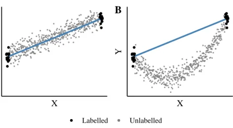
We now consider an application of the above mentioned strategy for subset selection in two hypothetical scenarios depicted in Figure 3.1. The first scenario is an example where the true relationship betweenXandY indeed is linear, and the second where the true model is quadratic. In both cases, the model seems to fit the data in the labelled subset very well, with no apparent devi-ations from the specified assumptions of linearity and homoscedasticity. In the second case, however, the fitted model produces disastrous predictions for the responsesyiin the underlying datasetD. Moreover, even though adding a quadratic term in theory would remove the bias, resorting to a quadratic model after subset selection is not only discouraged by the observed data but does not improve predictive performance either (Figure 3.2). Thus, using optimal design theory to deterministically select a subset from a large pool of instances, we may not be able to verify nor falsify the assumptions based on which the ’optimal’ subset was chosen. Furthermore, the problems induced by deterministic subset selection for misspecified models are present not only in simple linear regression models but for inference and prediction problems in general, and do not necessarily vanish with increasing sample sizes; see e.g. Shimodaira (2000); Sugiyama (2006); Bach (2007) and Sugiyama and Nakajima (2009).

3.3. Robustness against model misspecification 21

X

Y

A

X

Y

B

Figure 3.1:Deterministic subset selection ofn= 30instances from a pool ofN = 500

instances, optimised to minimise the variance of the estimator of the slope of a linear model. The y-values are observed only for the labelled sample (black), and remain unknown for the unlabelled data points (gray). A: the true model is linear. B: the true model is quadratic. The model seems to fit the data in the labelled subset very well in both cases, but has poor predictive performance when the model is misspecified.

X

Y

Figure 3.2: Deterministic subset selection ofn = 30instances (black) from a pool of

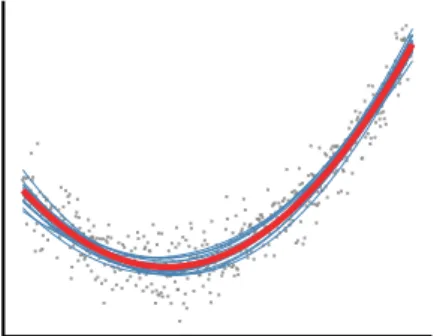
N = 500instances (gray), optimised to minimise the variance of the estimator of the slope of a linear model. Resorting to a quadratic model (red dotted line) after subset selection does not improve predictive performance.

3.3.2

The design-based approach

In this thesis, we have presented an alternative to subset selection that uses a random mechanism for sample selection that overcomes the deficiencies with model-based inference for misspecified models under dataset shift demon-strated above. Using random sampling and inverse probability weighing, we may actually control the selection mechanism and properly account for the induced selection bias, producing valid inference for the underlying database even under the realistic assumption of model misspecification. Indeed, robust-ness against model misspecification has been highlighted as one of the main strengths of sampling-weighted inference (Pfeffermann, 1993).

Returning to the example above, by the theory presented in Section 3.1 we obtain that the optimal sampling scheme for estimating the slopeβ1of a linear model, using random sampling with inverse probability weighting, is to choose

πi ∝ |xi−x¯|, wherex¯is the sample mean of thexi’s in the entire database D. Applying this sampling scheme to the datasets depicted in Figure 3.1, we obtain, on repeated subsampling, the results presented in Figure 3.3. In the first scenario, where the model is correctly specified, random sampling and deterministic selection produce similar results, although random sampling nat-urally introduces additional variation in estimating the regression line (Figure 3.1 A and 3.3 A). In the second case where the model is misspecified (Figure 3.1 B and 3.3 B), the results differ dramatically. In particular, random sampling produces substantially more accurate predictions than the ones obtained by deterministic instance selection, the reason being that the sampling-weighted estimator still estimates a well defined quantity, namely the ’best’ linear ap-proximation of the true relationship betweenX andY, where ’best’ is defined as the model we would obtain if all the data inDwere used. Furthermore, by use of random sampling it is possible to detect and adjust for modelling errors, so that accurate models may be developed (Figure 3.4).

3.3. Robustness against model misspecification 23

X

Y

A

X

Y

B

Linear fit on subsample Optimal linear fit

Figure 3.3: Estimated regression lines for 15 randomly selected samples ofn = 30

instances from a pool ofN = 500instances, optimised to minimise the variance of the sampling-weighted least squares estimator of the slope of a linear model. A: the true model is linear. B: the true model is quadratic. In both cases, the sampling-weighted estimator consistently estimates the regression line that would have been obtained if the entire database had been used.

X

Y

Quadratic fit on subsample True model

Figure 3.4: Estimated regression lines for 15 randomly selected samples ofn = 30

instances from a pool ofN = 500instances, optimised to minimise the variance of the sampling-weighted least squares estimator of the slope of a linear model. Correcting for modelling errors of the linear fit by adding a quadratic term produces consistent estimates of the true model from which the data was generated.

3.3.3

Design-based inference and robustness against model

misspecification

With the above example in mind, we repeat once again some of the key proper-ties of the proposed inferential procedure. First, we recall thatθˆπis a consistent estimator of the finite population parameterθ0under general regularity condi-tions (Binder, 1983). Although not formally proven, we expect the same to hold also forˆθt; see e.g. Yuan and Jennrich (1998) and the discussion concluding Chapter 3.2. Here, we may think ofθ0as the best approximation within the familyfθ(y|x)of the true relationship betweenXandY, in the sense that it

minimises the population loss`0(θ); clearly, we do not expect to do better than this based on a subsetS ⊂ D.

In contrast to model-based inference, where the validity of inferences drawn from a collected sample hinge on the correctness of the modelling assumptions, inference from ˆθπ andˆθtregarding the finite population parameterθ0 are solely design-based. Thus, the statistical properties of these estimators are determined completely by the sampling design, which is under direct control of the investigator, and is, with respect to inference regardingθ0, free of modelling assumptions. In particular,θˆπandˆθtremain consistent forθ0even under the realistic assumption of model misspecification, i.e when there are discrepancies between the analytic modelfθ(y|x)and the true data generating mechanism.

As another interesting feature, we note that the optimal sampling schemes given by Equation (3.1) – (3.3) in Section 3.1 also are design-based and don’t depend on the correctness of the assumed model. That is, irrespective whether the modelfθ(y|x)is correct or not, there exists an optimal sampling scheme in the sense that the asymptotic average variance of a collection of linear combinations ofˆθπandθˆtis minimised. However, the true optimal sampling scheme depends on unmeasured variables and additionally on the unknown optimal parameterθ0, and will, in any realistic application, remain unknown. Thus, in practical problems and applications, effort should be spent on finding good approximations to this unknown optimum.

4 Summary of papers

4.1

Paper I

Introduction

We consider a statistical learning problem of estimating a parameterθ of a statistical modelfθ(y|x)from a subset of a random sample(xi, yi), i= 1, . . . , N, with the aim of obtaining a predictive modelfθˆ(y|x). The predictorsxiare known for all members of the initial sample, but the outcomesyiare observable only for a smaller subset. We consider the task of optimal sampling for selection of the subset for which the responsesY will be observed.

Active learning

We present an active learning algorithm that sequentially samples new in-stances at random from a large pool of available inin-stances, updating the current estimateˆθtof the parameterθby minimisation of a sampling-weighted loss function. Our active learning algorithm extends the finite population sampling methodology to a sequential sampling framework that iteratively samples new instances, and extends existing unbiased active learning algorithms from selecting one instance at a time to randomised batch-sampling.

Optimal sampling schemes

We consider a twice differentiable loss function and a general class of regular statistical models, for which the expectation ofYigivenxican be expressed in terms of a differentiable functionµ : _R → RasEθ[Yi|xi] = µ(xTiθ). We

show that both the mean squared error of the predictions{µ(xT

i ˆθt)}Ni=1and the variance of the total loss`0(ˆθt)admits asymptotic expansions of the form

k1 t X s=1 N X i=1 ci(θ0) πs(i) +k2+o(n−1) ,

where k1 and k2 are constants not depending on the vectorsπ1, . . . ,πt of sampling probabilities, andci(θ0)are quadratic expressions depending on {(xi, yi)}Ni=1andθ0. Moreover, the first term of the above expression is min-imised by choosing sampling probabilities according to

πs(i)∝ p

ci(θ0) , normalised so thatPNi=1πs(i) = 1.

We further propose approximation of the optimal sampling schemes by re-placing the unknown optimal coefficientsci(θ0) with their corresponding expectations, evaluated at the current parameter estimateθˆt, and show that the resulting sampling schemes have a close connection to to statistical leverage, a commonly used influence measure in generalised linear regression mod-elling (Pregibon, 1981). Practically speaking, this means that optimal predictive performance is achieved by oversampling highly influential instances, and by oversampling data points with a large influence on the predictions per-taining to uncertain instances in particular. For classification problems, this corresponds to oversampling instances that are influential for detection of the decision boundary.

Results

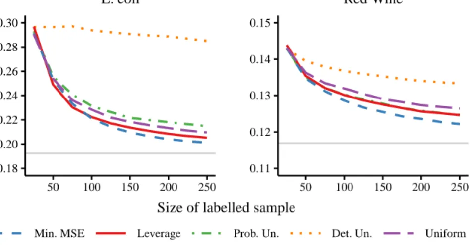
An empirical evaluation of the proposed active sampling schemes demon-strated improved predictive performance, both compared to simple random sampling and to various instance selection procedures previously suggested in the literature (Figure 4.1).

4.1. Paper I 27 0.18 0.20 0.22 0.24 0.26 0.28 0.30 50 100 150 200 250 Misclassif ication rate E. coli 0.11 0.12 0.13 0.14 0.15 50 100 150 200 250 Red Wine

Size of labelled sample

Min. MSE Leverage Prob. Un. Det. Un. Uniform

Figure 4.1: Performance of five different sampling schemes for on two benchmark datasets, using schemes sampling optimised to minimise the mean squared error (MSE) of the predictions, sampling proportional to the square root of the statistical leverage score, probabilistic uncertainty sampling (Chu et al., 2011; Ganti and Gray, 2012), deter-ministic uncertainty sampling (Lewis and Gale, 1994), and uniform random sampling. The gray solid line represents the misclassification rate using the entire dataset for training.

Conclusions

We have derived optimal sampling schemes for unbiased active learning, in the sense that the variance of the total loss and the mean squared error of the predictions are minimised. Our empirical results demonstrate better predictive performance than competing methods on a number of benchmark datasets. In contrast, deterministic uncertainty sampling (Lewis and Gale, 1994) always performed worse than simple random sampling, as did uncertainty-based random sampling in one of the examples. To conclude, our study shows that sample selection in unbiased active learning should not target the most uncertain instances, as previously have been suggested (Chu et al., 2011; Ganti and Gray, 2012), but the most influential ones.

4.2

Paper II

Introduction

A huge challenge in the analysis of naturalistic driving data is making efficient use of the overwhelming amounts of information stored in naturalistic driving study (NDS) databases. The great cost associated with video annotation often required for statistical analyses implies that data analysis must be restricted to a limited subset of the original database. Thus, choosing this subset in a manner that captures as much of the available information as possible is essential. In this paper, we show how sample selection may be optimised using information readily available in the database through automatic recordings of vehicle manoeuvre data. The methodology is consequently illustrated using data collected in Sweden as part of the European large scale field operational test (euroFOT) study (Kessler et al., 2012).

Methods

We consider a traffic situation involving two vehicles, the vehicle taking part in the NDS study (the index car) and a front car. The two are driving at similar speeds, when the front car brakes. This scenario describes a situation where a potential safety critical event (SCE) can occur, namely a rear-end collision. Of interest is the question of whether the glancing behaviour of the driver of the index car, namely whether he/she looks at the car in front when braking is initiated, and the speed of the vehicles and time gap between the two cars at this initiation, have an impact on the likelihood that a safety critical event will occur.

To answer this question, we consider a logistic regression model

logitP(Y = 1|X) =θ0+θ1Time gap+θ2Speed+θ3Glance

+θ4Glance∗Time gap ,

(4.1)

whereY is a binary variable indicating whether a safety critical event occurred in a specific driving instance or not, Time gap is the distance between the vehicles measured in seconds, andGlanceis a binary indicator whether the driver is having eyes-off-road at brake light.

4.2. Paper II 29

Optimal sampling schemes

Considering a cohort of 49 SCEs and 500 non-SCEs and the logistic regres-sion model (4.1), we used auxiliary information readily available in the NDS database to compute optimal sampling schemes with respect to various linear optimality criteria. Generally, controls at high anticipated risk of SCE were oversampled, i.e controls driving at high speed, small time gap, and with a high predicted tendency of glancing off road. Relatively large sampling probabilities were also assigned to controls at moderate to mild risk, constituting a subset to which the characteristics of the cases and high risk controls may be contrasted. Controls at low risk tended to be selected with low probability, as these are anticipated to contribute with little information with regards to safety.

Results

Poisson sampling optimised for a specific linear combination of parameters generally resulted in an increased precision of the corresponding parameter estimates, as compared to simple random sampling, and the gain in precision increased with the size of the control sample. With n = 50controls, the standard deviation (SD) of the estimator for the effect of time gap was reduced by 12% using instance selection optimised for this particular parameter. The corresponding information loss, measured as increase in SD compared to analysing the entire database, was 74%. Atn= 200, the results were improved further to an SD reduction of 31% compared to SRS. In this case, using 40% of the database resulted in only 24% loss of information. Similar results were observed also for optimisation with respect to the effect of vehicle speed. On the contrary, only limited auxiliary information for glancing was available, and linear combinations involving glancing were consequently poorly estimated, particularly at small sample sizes.

Conclusions

We have presented an inferential framework for the analysis of large NDS databases in which complete data collection is costly, and shown how instance selection in naturalistic driving data may be optimised by the use of auxil-iary information readily available for all instances in an NDS database. We have illustrated through a case study how such sampling designs may be implemented in practice, and demonstrated that a substantial gain in statistical efficiency may be achieved when good auxiliary information and proxies for the variables on interest are available.

Bibliography

Atkinson, A. C. and Donev, A. N. (1992). Optimum Experimental Designs. Clarendon Press, Oxford, England.

Bach, F. R. (2007). Active learning for misspecified generalized linear models. In

Advances in Neural Information Processing Systems 19.

Binder, D. A. (1983). On the variances of asymptotically normal estimators from complex surveys.International Statistical Review, 51(3):279–292.

Chu, W., Zinkevich, M., Li, L., Thomas, A., and Tseng, B. (2011). Unbiased online active learning in data streams. InProceedings of the 17th ACM SIGKDD Conference on Knowledge Discovery and Data Mining.

DasGupta, A. (2008).Asymptotic Theory of Statistics and Probability. Springer, New York, NY.

Fishman, G. S. (1996).Monte Carlo. Springer, New York, NY. Fuller, W. A. (2009).Sampling Statistics. Wiley, Hoboken, NJ.

Ganti, R. and Gray, A. (2012). UPAL: Unbiased pool based active learning. InProceedings of the 15th International Conference on Artificial Intelligence and Statistics.

Hansen, M. H. and Hurwitz, W. N. (1943). On the theory of sampling from finite populations.The Annals of Mathematical Statistics, 14(4):333–362.

Hartley, H. O. and Sielken, R. L. (1975). A "super-population viewpoint" for finite population sampling.Biometrics, 31(2):411–422.

Horvitz, D. G. and Thompson, D. J. (1952). A generalization of sampling without replacement from a finite universe. Journal of the American Statistical Association, 47(260):663–685.

Huber, P. J. and Ronchetti, E. M. (2009).Robust Statistics. Wiley, Hoboken, NJ.

Kessler, C., Etemad, A., Alessandretti, G., Heinig, K., Selpi, Brouwer, R., Cserpinszky, A., Hagleitner, W., and Benmimoun, M. (2012). EuroFOT Deliverable D11.3 Final Report. Project deliverable, euroFOT consortium, Aachen, Germany.

Lewis, D. D. and Gale, W. A. (1994). A sequential algorithm for training text classifiers. InProceedings of the 17th Annual International ACM SIGIR Conference on Research and Development in Information Retrieval.

Ma, P., Mahoney, M. W., and Yu, B. (2014). A statistical perspective on algorithmic leveraging. InProceedings of the 31 st International Conference on Machine Learning. Ma, P., Mahoney, M. W., and Yu, B. (2015). A statistical perspective on algorithmic

leveraging.Journal of Machine Learning Research, 16:861–911.

Ma, P. and Sun, X. (2015). Leveraging for big data regression. Wiley Interdisciplinary Reviews: Computational Statistics, 7(1):70–76.

McCullagh, P. and Nelder, J. A. (1989). Generalized Linear Models. Chapman & Hall, London, England.

Pfeffermann, D. (1993). The role of sampling weights when modeling survey data.

International Statistical Review, 61(2):317–337.

Pregibon, D. (1981). Logistic regression diagnostics.The Annals of Statistics, 9(4):705–724. Rubin-Bleuer, S. and Schiopu Kratina, I. (2005). On the two-phase framework for joint

model and design-based inference.The Annals of Statistics, 33(6):2789–2810.

Särndal, C. E., Swensson, B., and Wretman, J. (2003). Model Assisted Survey Sampling. Springer, New York, NY.

Settles, B. (2012). Active learning.Synthesis Lectures on Artificial Intelligence and Machine Learning, 6(1):1–114.

Shimodaira, H. (2000). Improving predictive inference under covariate shift by weight-ing the log-likelihood function.Journal of Statistical Planning and Inference, 90:227–244. Skinner, C. J. (1989). Domain Means, Regression and Multivariate Analysis. In Skinner, C. J., Holt, D., and Smith, T. M. F. (Eds.),Analysis of Complex Surveys, pp. 80–87. Wiley, New York, NY.

Sugiyama, M. (2006). Active learning in approximately linear regression based on conditional expectation of generalization error.Journal of Machine Learning Research, 7:141–166.

Sugiyama, M. and Nakajima, S. (2009). Pool-based active learning in approximate linear regression.Machine Learning, 75:249–274.

Tillé, Y. (2006).Sampling Algorithms. Springer, New York, NY.

Yuan, K. H. and Jennrich, R. I. (1998). Asymptotics of estimating equations under natural conditions.Journal of Multivariate Analysis, 65:245–260.