Generating large scale images using GANs

(1)

American University in Cairo American University in Cairo

AUC Knowledge Fountain

Theses and Dissertations

2-1-2019

Generating large scale images using GANs

Mohamed Mohsen Mahmoud Mohamed

Follow this and additional works at: https://fount.aucegypt.edu/etds

Recommended Citation Recommended Citation

APA Citation

Mohamed, M. (2019).Generating large scale images using GANs [Master’s thesis, the American University in Cairo]. AUC Knowledge Fountain.

https://fount.aucegypt.edu/etds/724

MLA Citation

Mohamed, Mohamed Mohsen Mahmoud. Generating large scale images using GANs. 2019. American University in Cairo, Master's thesis. AUC Knowledge Fountain.

(2)

Generating Large Scale Images Using GANs

Mohamed Mohsen American University in Cairo, [email protected]

Advisor: Prof. Mohamed Moustafa

This thesis is submitted as a part of the requirements of the Masters of Science in Computer Science Program

(3)

Acknowledgements

I would first like to thank my thesis advisor Professor Mohamed Moustafa

for his continuous support throughout this thesis. Whenever I needed

guid-ance, he steered me in the right direction and bared with me the couple of

times we changed the thesis topic.

I would also like to thank my thesis committee for generously devoting

the time to provide the required support and guidance throughout the review

of this document.

I would also like to thank my managers and colleagues in Microsoft for

their flexibility and continuous support. They were always pushing me to

finish my thesis and gave me the time required to finalize my work when I

needed it the most.

I am especially thankful to my wife Sohair Osama, my parents Mohsen

Mahmoud and Basma Abdelrahman, my sister Heba Mohsen, my brother

Ahmed Mohsen, my aunt Iman Abdelrahman, my parents-in-law Osama

Alatroush and Mona Gamal and my friends for their continuous support

throughout my work on this degree. They gave me the push to finish this

work when I most needed it. This work would not have been possible without

them. Thank you.

Author

(4)

List of Figures

1 Deep Convolutional GAN . . . 7

2 Laplacian Pyramid Architecture . . . 8

3 Deep Recurrent Attention Writer in Action . . . 9

4 Super-resolution GAN Architecture . . . 10

5 Sample results for image hole filling . . . 11

6 Sample results for image denoising . . . 12

7 Block diagram for the separate training approach . . . 15

8 Block diagram for the joint training approach . . . 16

9 Block diagram for the combined network approach . . . 17

10 Baseline Generator architecture used . . . 20

11 Baseline Discriminator architecture used . . . 20

12 Generator architecture used . . . 21

13 Discriminator architecture used . . . 21

14 Samples from generator network . . . 22

(7)

16 64x64 pixel samples from the super resolution network

(scal-ing factor 2x) . . . 24

17 128x128 pixel samples from the super resolution network (scal-ing factor 4x) . . . 25

18 64x64 pixel samples from the combined networks . . . 27

19 128x128 pixel samples from the combined networks . . . 28

20 Sample results for the joint training approach . . . 29

(8)

List of Tables

1 Evaluation of super resolution network . . . 26

(9)

I

Abstract

Generative Adversarial Networks [1] have been used for the task of

im-age generation and has achieved impressive results [2][3]. There is always

a challenge to train networks that generate large scale images since they

tend to be huge and training needs a lot of data. In this work, we tackle

this problem by dividing it into two smaller parts. We first generate small

scale images using GANs then use a super resolution network to enlarge the

generated images resulting in large scale images. Using a super resolution

network helps in adding more details to the image which results in a better

quality image. This technique has been tested with a small amount of data

(10)

II

Introduction

In modern days, the amount of data available to train machine learning

algorithms is getting larger, however, the cost of labeling is expensive. Many

of the machine learning approaches require annotated data for training and

testing, therefore, the need for labeled data is growing. One of the solutions

for this problem is to use generated data for training instead of real data.

One of the prominent approaches for image generation is using the

Gen-erative Adversarial Networks [1]. Since GANs make use of two deep networks

that should be trained simultaneously, they are difficult to train. Work has

been done to try and regularize the GANs training [2][3]. However, the

images generated are still small in size (less than 128x128 pixels).

A different stream of work that is tackled using GANs is the image

super-resolution problem [4][5]. This is where the input is a low super-resolution image

and the output is the higher resolution version. This makes use of unlabeled

data. Where a large scale image is downsized and used for the input while

the large scale image is used as a reference for the output.

For this work, we will focus on the task of large scale image generation by

exploring the joint training of GANs along with a super-resolution network.

We explore the different ways of combining super-resolution networks with

generative networks. Our proposed system achieves better results over a

(11)

Section III provides a more detailed description of the problem tackled.

A review of current work is presented in section IV. The approach is

demon-strated in section V. Section VI describes the experiments performed and

their results. The conclusion is found in section VII and possible future

(12)

III

Problem Definition

Image generation is not an easy problem. Trying to generate large scale

images add complexity to the generation. Complex networks with high

dimensionality inputs and outputs are not easy to train. In this work, we

tackle this problem by providing a way to generate larger images. This is

done by exploring the different ways to integrate a super-resolution network

(13)

IV

Literature Survey

IV.1 Generative Adversarial Networks (GANs)

GANs offer a technique for data generation that is based on adversarial

learning [1]. This technique trains two networks simultaneously, a generator

and discriminator network are trained in parallel. The goal of the generator

is to fool the discriminator into thinking that a generated image is real.

While the goal of the discriminator is to identify real vs fake images. As

training progresses, the generator generates more real looking images and

the discriminator gets better at detecting fake images [1].

Training GANs is a very challenging problem because instead of only

training a single network, one has to train the generator and the

discrimina-tor networks simultaneously. Also, for the training to be successful, one has

to make sure that the generator and discriminator are trained at the same

speed i.e. the learning capacity of the networks is similar. If the

discrimi-nator learns faster than the generator, the whole process is affected and the

generator stops learning.

The inherited difficulty and complexity of GANs make them difficult to

(14)

IV.2 Deep Convolutional GANs (DCGANs)

Convolutional Neural Networks (CNNs) have shown remarkable results

in the different image classification problems. Work has been done to scale

up the learning capacity of GANs by making use of Deep Convolutional

Networks [2]. The authors came up with a set of architecture guidelines for

stable training of DCGANs [2]. They also suggest using the Adam optimizer

[6] for the training. This approach results in plausible image generation when

trained on the LSUN dataset [7].

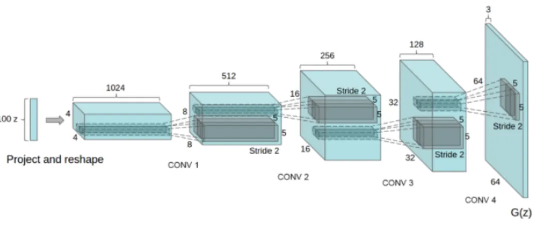
The network uses strided convolutions as shown in figure 1. There are

a total of 4 convolutional layers with a 100 dimensional input vector and

a 64x64 rgb output image. This work shows the power of using deep

con-volutional networks in GANs however, the images generated are not high

resolution images.

This approach increases the learning power of GANs and thus improves

the quality of output images generated by them. However, the deeper and

the more complex the network gets, the more tricky it is to train.

IV.3 Laplacian Pyramid Approach (LAPGAN)

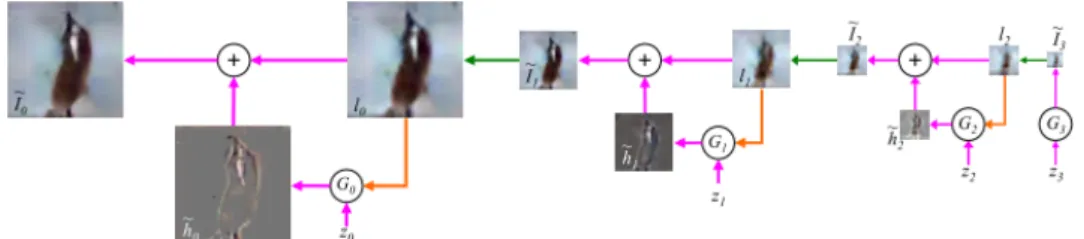
One of the approaches to train GANs is to use a Laplacian pyramid

of Adversarial Networks [3]. This means divides the training problem into

smaller subproblems. As shown in figure 2, a series of Conditional

(15)

Figure 1: Deep Convolutional GAN

The architecture of the DCGAN generator network. The input is a 100 dimensional vector and the generated images are 64x64 color images. Image adopted from [2]

layer learns the differential to add to the input image for refinement. The

refined image is then upscaled and moves on to the next CGAN block. The

first block is a normal GAN [1] that generates a small scale image with an

input of a noise vector.

This work makes use of the fact that each CGAN layer is only learning

the differential to add to the input image instead of learning to generate

the image from scratch. LAPGANs were tested on the CIFAR10 [9], STL10

[10] and LSUN [7] datasets and their results show an improvement over the

traditional GAN approach. Human evaluation was done to come with this

conclusion [3]. Images generated using this approach have a dimension of

64x64 pixels.

The success of this approach is due to the fact that it trains for the

differential to improve the image quality. This decreases the amount of data

(16)

Figure 2: Laplacian Pyramid Architecture

The architecture of the LAPGAN generator network. Green arrows represent the up-sampling of the images generated at a specific stage to form the input to the next stage. Image adopted from [3]

each layer easier. All of this leads to better quality output images.

IV.4 Deep Recurrent Attention Writer (DRAW)

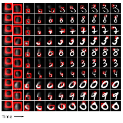
When drawing, we humans tend to focus on a small part of the picture

at a time and then move on to the next part of the picture. This is modeled

using the attention mechanism [11]. The network chooses a small part of the

image to attend to at a time. A Gaussian kernel composed of a variational

auto encoder is used to generate part under focus. Figure 3 demonstrates

the power of this algorithm in following lines and recursively refining images

generated from the MNIST data [12].

This whole operation is done in a recurrent fashion. Where the area

at-tended to keeps getting smaller as more details are added to the image. This

technique [11] is shown to work on generating MNIST [12] and SVHN [13]

data. However, when generation was tested with the CIFAR10 [9] dataset,

the images produced capture much of the shape structure but are blurred

(17)

The success of this approach in generating numerical images and it’s

failure to generate scenery is because of the fact that it focuses on a small

part of the picture at a time, this is good when it comes to tracing lines and

thus generating numbers. However, scenery images do not have the same

structure and thus this approach fails to generate acceptable images in this

scenery images.

Figure 3: Deep Recurrent Attention Writer in Action

The DRAW generator in action. The red squares represent the area of attention of the algorithm. As seen, the algorithm is good at following lines and recursively refining the image. This image is adopted from [11]

(18)

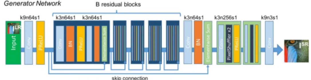
Figure 4: Super-resolution GAN Architecture

The architecture of the SRGAN generator network. As seen, the input images have a dimension of 64x64 pixels and are upscaled with a 4x factor to generate images of 256x256 pixels. Image adopted from [4]

IV.5 Super-resolution GAN (SRGAN)

The use of GANs for super-resolution is demonstrated by SRGAN [4].

This approach trains the discriminator on separating between the original

and fake high-resolution images. On the other hand, the generator takes in

a low-resolution image and generates the high-resolution version. Figure 4

shows the architecture of the SRGAN generator network.

In addition the output of the discriminator, the generator optimizes for

the VGG [14] features loss for the generated and original high-resolution

images. Using this loss function, the authors could successfully upscale

images with a 4x scaling factor.

This technique produces larger scale images (256x256 pixels) than the

previously described algorithms. However, it needs a low resolution image

(64x64 pixels) as input.

Since this approach uses a very deep and complex super resolution

(19)

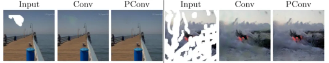
Figure 5: Sample results for image hole filling

This picture shows a comparison between the use of typical convolution layer based networks vs partial convolution layers in solving the problem of hole filling. Image adopted from [15]

IV.6 Image Denoising Networks

Denoising is the problem of removing noise from images or filling in

holes in the image. This problem has been tackled by various learning and

non-learning techniques. In our scenario, we are more interested about the

learning techniques.

The use of partial convolution layers [15] has been explored and it has

shown great results in filling gaps in images. It has been testing by applying

arbitrary shaped hole masks to images and then try to fill in the gaps.

The partial convolution yielded far superior results when compared to the

convolutional networks an example is shown in figure 5.

Another approach that focuses on noise removal is presented in [16].

They have developed a convolutional network with skip connections to

elim-inate the noise and improve the image quality. A sample of the output is

shown in figure 6.

(20)

Figure 6: Sample results for image denoising

This picture shows sample outputs of the denoising network. The image on the left is the input image with noise and the image on the right is the corresponding enhanced version. Image adopted from [16]

(21)

in [16]. The main problem is that denoising systems expect the input and

output to be of the same resolution. As a workaround, the low resolution

image is upscaled and then fed in the denoising network. By doing this, the

overall system would be taking in a low resolution image and outputting a

(22)

V

Proposed Solution: Combining Super

Resolu-tion with GAN

Motivated by the ability of super-resolution networks to produce 8x

higher resolution images, we have explored the different ways to combine

a super-resolution network along with a GAN network. Super-resolution

networks need a pair or low-resolution and high-resolution images to train

where the GAN only needs a random vector. Below are the different

ap-proaches to combine the two systems.

V.1 Approach 1: Separate Training

The first way to combine the systems, is by separately training the

super-resolution network and the GAN on the same dataset. Where the GAN

would be trained to generate low-resolution images and the super-resolution

network would separately learn to enlarge low-resolution images from the

same dataset. Taking the output of the GAN and feeding it in the

super-resolution network should produce high-super-resolution images. Figure 7 shows

a block diagram of this approach.

V.2 Approach 2: Joint Training

The second approach is to train the super-resolution network on the

(23)

Figure 7: Block diagram for the separate training approach

The GAN and Super resolution networks are trained separately and when generat-ing, the output of the generator network is fed in the super resolution network to obtain the large scale image.

approach. This approach aims at adapting the super-resolution network to

the images generated from the GAN. The training steps are outlined below:

1. Train the GAN to generate low-resolution images. This steps

makes use of the power of GANs in generating low-resolution images.

2. Find the closest image from the training dataset. Super-resolution

networks need pairs of low-resolution images along with their

high-resolution counterparts. The GAN already generated the low-high-resolution

version but we still need to find the corresponding high-resolution

im-age. Therefore, we search the training dataset to find the closest image

and use its high-resolution version.

3. Train the super-resolution network. Making use of the

(24)

counter-Figure 8: Block diagram for the joint training approach

After the GAN network is trained, training data for the super resolution network is created by generating random images and matching them with the nearest large scale corresponding image from the dataset.

part from the dataset, train the super-resolution network.

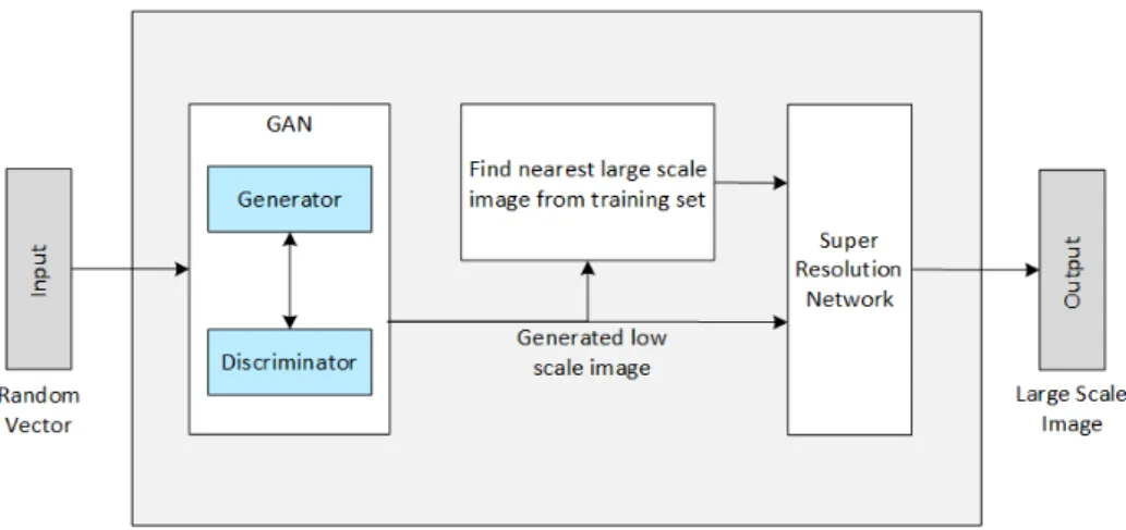
V.3 Approach 3: Combined Network

One further step in integrating the super-resolution network with the

GAN would be to train them together. The high level block diagram is

shown in figure 9. This approach makes use of the error from the

super-resolution network to train the generator of the GAN. The training steps

for each epoch are described below:

1. Generate a low-resolution image. Use the generator network from

the GAN to generate an image.

2. Find the closest image from the training dataset. Search the

(25)

Figure 9: Block diagram for the combined network approach

The error from the super resolution network is used by the generator network to adapt.

3. Enlarge image using super-resolution network. Use the super

resolution network to increase the image resolution.

4. Consume the error from the super-resolution network to train

the generator. This is the key step, error from the super-resolution

network should be fed back to train the generator as well as the

(26)

VI

Experiments

VI.1 Dataset Used

All training was done on the LSUN dataset[7] using the ‘church outdoor’

category. This is the smallest category in the dataset and contains:

• 126,227 training image

• 300 validation image

The images in the dataset do not have a uniform size. All samples

have their smaller dimension equal to 256 pixels or larger. The following

preprocessing steps were done in order to prepare the images:

1. Crop the largest center square of each image

2. Shrink the cropped portion to the required size

VI.2 Evaluation Metrics

Inception Score

Evaluating generative models is a very difficult task since there is no

ground truth to compare to. For that reason, researchers mostly rely on the

human perception of the generated image quality. Recent work proposed a

(27)

image quality. It has shown to correlate well with the human perception of

the image quality.

To evaluate the output of generative models, the inception score aims at

measuring two things:

1. The clarity of the objects in the generated images

2. The diversity of the generated images

A classifier model is pre-trained on the imagenet dataset [19] and is used

in the standard inception score calculation. This model is the core of the

calculation, the clarity and diversity of the objects in the generated images

are measured by measuring the output of the classifier for the different

classes of the classifier.

Structural Similarity

Structural similarity [20] computes the similarity between images by

us-ing groups of pixels instead of individual pixels. It takes into consideration

the luminance, contrast and image structure in the similarity computation.

This is one of the metrics that we have used to find the nearest image in the

training set given a generated image.

VI.3 Baseline Approach

(28)

Figure 10: Baseline Generator architecture used

The architecture of the generator network for the baseline approach. As seen, the input is a random vector of size 100. Multiple convolutional layers turn that input to an image of size 64x64.

Figure 11: Baseline Discriminator architecture used

The architecture of the discriminator network for the baseline approach. As shown, the input is a 64x64 pixel image and the output is a single value that indicates if the image is authentic or fake.

work, we will use an adapted version of the deep convolutional GAN [2] to

generate large scale images and compare them with the ones generated using

our proposed approaches. The generator network architecture is shown in

figure 10 and the discriminator network architecture is shown in figure 11.

This model is trained with a batch size of 512 images and using the

Adam Optimizer[6] with learning rate of 0.0005 for 50,000 epochs. Results

(29)

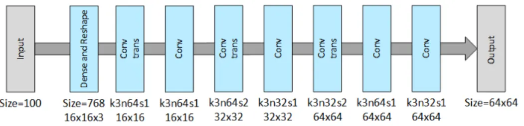
Figure 12: Generator architecture used

The architecture of the generator network used. As seen, the input is a random vector of size 100. Multiple convolutional layers turn that input to an image of size 32x32.

Figure 13: Discriminator architecture used

The architecture of the discriminator network used. As shown, the input is a 32x32 pixel image and the output is a single value that indicates if the image is authentic or fake.

VI.4 Approach 1: Separate Training

Generative Adversarial Network

A deep convolutional GAN is trained to generate 32x32 pixels images.

The architecture of the generator network is outlined in figure 12 and the

architecture of the discriminator network is outlined in figure 13.

After training various GAN models, it was noticed that the most

impor-tant thing to take care of while training is that the generator and

discrimi-nator networks need to be learning with the same speed. It is quiet easy to

(30)

Figure 14: Samples from generator network

Those are 32x32 image samples from the generator network. As noticed, the images do indeed look like churches and some of the samples can be mistaken as real images even by a human eye.

between fake and authentic images. However, such a discriminator results in

the generator not being able to keep up and thus it doesn’t learn anything.

Therefore, the size of the discriminator network is tweaked to maintain an

accuracy of 80% to 90% for the discriminator. This is the sign of a healthy

training.

The model is trained with a batch size of 512 images using the Adam

Optimizer[6] with a learning rate of 0.0005 for 50,000 epochs. A sample

output is shown in figure 14.

Super Resolution network

Different super resolution network architectures are tried out on the

training data and the one that produced the best SNR is the Denoising

(31)

Figure 15: Super resolution architecture used

The architecture of the denoising super resolution network used. As seen, the input is a 128x128 image and the output is also a 128x128 image.

The denoising network is initially meant to remove noise from images

without changing their size. To use a denoising network to enlarge images,

a preprocessing step is added to stretch the image using the bilinear

inter-polation before feeding it to the denoising network. Therefore, the whole

system would take in a 32x32 image and output the large scale image. The

same idea is presented in [16].

Training is done using a batch size of 1 and the Adam optimizer[6] with

a learning rate of 0.00001. The optimization function used is the mean

square error. The training evaluation is shown in table 1. Examples from

(32)

Figure 16: 64x64 pixel samples from the super resolution network (scaling factor 2x)

The top row is the 32x32 input image, the second row is a stretched version using bilinear interpolation for comparison. The third row is the 64x64 output of the network while the last row is the original large scale image. This network obtained a PSNR of -18.8 on the validation set.

(33)

Figure 17: 128x128 pixel samples from the super resolution network (scaling factor 4x)

The top row is the 32x32 input image, the second row is a stretched version using bilinear interpolation for comparison. The third row is the 128x128 output of the network while the last row is the original large scale image. This network obtained

(34)

Scaling factor Output Dimensions PSNR

2x 64x64 -18.8

4x 128x128 -22.24

Table 1: Evaluation of super resolution network

PSNR values are calculated on the validation set.

Combined Result

Feeding the output of the generator into the super resolution networks,

gives us 64x64 or 128x128 generated images depending on the super

resolu-tion network used. Figures 18 & 19 show samples of images that are

gener-ated using the combination of the GAN and the super resolution networks.

The super resolution network succeeds in clearly improving the quality of

the enlarged version over the bilinear interpolation by adding some missing

details to the images.

VI.5 Approaches 2&3: Joint Training & Combined Network

These approaches depends on generating images and then finding similar

images from the training set to train the super resolution network. We have

tried out different similarity and error metrics in order to find the nearest

image from the training set.

From the sample results shown in figure 20, we can notice that after

(35)

Figure 18: 64x64 pixel samples from the combined networks

The top row is the 32x32 image generated by the generator network. The second row is the stretched version using bilinear interpolation for comparison. The third row is the result of feeding the generator image to the super resolution network to generate a 64x64 version. As noticed, even tough a human eye can tell that those images are not real, they are of very good quality for machine generated images.

After some debugging, we found out that the problem is that the input and

output images used to train the super resolution network are not correlated.

Since we are using a very diverse training dataset, for each similarity metric

a certain type of images dominate the results. Therefore, the nearest image

from the training set is mostly not similar to the generated image. Example

output for the different similarity metrics is shown in figure 21. Without the

ability to really find the most similar image in the training set, approaches

(36)

Figure 19: 128x128 pixel samples from the combined networks

The top row is the 32x32 image generated by the generator network. The second row is the stretched version using bilinear interpolation for comparison. The third row is the result of feeding the generator image to the super resolution network to generate a 128x128 version. As noticed, even tough a human eye can tell that those images are not real, they are of very good quality for machine generated images.

(37)

Figure 20: Sample results for the joint training approach

The top row is the 32x32 image generated by the generator network. The second row is the stretched version using bilinear interpolation for comparison. The third row is the result of feeding the generator image to the super resolution network to generate a 128x128 version. As noticed, after the super resolution network is applied, the images loose all of their details and are extremely blurred. Those samples are computed using the normalized mean square error.

(38)

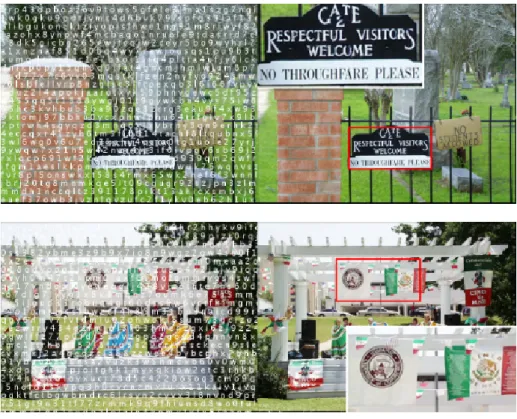
(a) (b) (c)

Figure 21: Similarity between generated images and training set

In each of the sub figures shown, the image on the left is a random generated image and the image on the right is the corresponding nearest image from the training set. Each of the sub figures, represents a different similarity/error measure sub figure 21a is computed using structural similarity [20] as the similarity measure. Sub figure 21b is computed using the normalized mean squared error as the error function. While sub figure 21c is computed using PSNR as the error measure.

VI.6 Comparison to Baseline

The baseline for this work is the quality of images generated using a

GAN network that is trained on the same dataset. To evaluate the baseline,

a GAN network of the same architecture outlined in figures 12 & 13 is trained

(39)

Training a network to generate 128x128 images using a single GAN is a

very compute intensive process that does not fit on the GPU memory. The

network will have to be stripped down for it to fit on a GPU which would

lead to a weaker network and thus misleading results. Therefore, we are

instead doing the comparison for 64x64 images.

For the sake of the comparison, the denoising super resolution network

shown in figure 15 is retrained to generate 64x64 images. In other words,

we needed to change the super resolution network scaling factor from 4x to

2x.

From the training difficulty point of view, the baseline requires a GAN

to generate higher dimensionality images and is thus much more difficult to

train. Using our approach, the network size is much smaller and thus the

training is much easier. Moreover, bigger networks require more data to

train. Therefore, our approach should work better with smaller datasets.

As noticed from table 2, our approach gives better inception score values

on average than the baseline. Which shows it is indeed better than the

(40)

Inception Score

Mean Standard Deviation

Baseline Convolutional GAN 3.041 0.110

Our Approach 3.564 0.220

Table 2: Comparison with the baseline

Calculated for a sample of 1024 generated image from each approach, the mean and standard deviation of the inception score are shown in the table.

(41)

VII

Conclusion

Based on the results obtained on this small dataset, combining a GAN

with a super resolution system proves more powerful in generating

bet-ter quality images in comparison to only using GAN. This is because the

proposed technique divides the problem into two smaller problems which

makes it more manageable. Also, since the problem is divided into smaller

problems, it is possible to use a very small training set of 126,227 images

(42)

VIII

Future Work

Although the current approach already achieved better results over the

baseline, there is room for improvement. An extension to the super

resolu-tion network is to train on more data e.g. the image net dataset[19] and then

adapt it to the domain. Also, noise should be added to the lower resolution

images used in training the super resolution network. This would resemble

the noisy images generated from the GAN which would lead to generating

(43)

Bibliography

[1] Ian J. Goodfellow, Jean Pouget-Abadie, Mehdi Mirza, Bing Xu, David

Warde-Farley, Sherjil Ozair, Aaron Courville, and Yoshua Bengio.

Gen-erative adversarial nets. In Proceedings of the 27th International

Con-ference on Neural Information Processing Systems - Volume 2, NIPS’14,

pages 2672–2680, Cambridge, MA, USA, 2014. MIT Press.

[2] Alec Radford, Luke Metz, and Soumith Chintala. Unsupervised

repre-sentation learning with deep convolutional generative adversarial

net-works. arXiv preprint arXiv:1511.06434v2, 2015.

[3] Emily L Denton, Soumith Chintala, arthur szlam, and Rob Fergus.

Deep generative image models using a laplacian pyramid of adversarial

networks. In C. Cortes, N. D. Lawrence, D. D. Lee, M. Sugiyama,

and R. Garnett, editors, Advances in Neural Information Processing

Systems 28, pages 1486–1494. Curran Associates, Inc., 2015.

(44)

Photo-realistic single image super-resolution using a generative

adver-sarial network. arXiv preprint arXiv:1609.04802v5, 2016.

[5] Wei-Sheng Lai, Jia-Bin Huang, Narendra Ahuja, and Ming-Hsuan

Yang. Deep laplacian pyramid networks for fast and accurate

super-resolution. arXiv preprint arXiv:1704.03915v2, 2017.

[6] Diederik P. Kingma and Jimmy Ba. Adam: A method for stochastic

optimization. InInternational Conference for Learning Representations

(ICLR), 2015.

[7] Fisher Yu, Yinda Zhang, Shuran Song, Ari Seff, and Jianxiong Xiao.

Lsun: Construction of a large-scale image dataset using deep learning

with humans in the loop. arXiv preprint arXiv:1506.03365, 2015.

[8] Mehdi Mirza and Simon Osindero. Conditional generative adversarial

nets. 11 2014.

[9] Alex Krizhevsky. Learning multiple layers of features from tiny images.

2009.

[10] Adam Coates, Andrew Ng, and Honglak Lee. An analysis of

single-layer networks in unsupervised feature learning. In Geoffrey Gordon,

David Dunson, and Miroslav Dudk, editors, Proceedings of the

(45)

volume 15 ofProceedings of Machine Learning Research, pages 215–223,

Fort Lauderdale, FL, USA, 11–13 Apr 2011. PMLR.

[11] Karol Gregor, Ivo Danihelka, Alex Graves, Danilo Rezende, and Daan

Wierstra. Draw: A recurrent neural network for image generation. In

Francis Bach and David Blei, editors, Proceedings of the 32nd

Inter-national Conference on Machine Learning, volume 37 ofProceedings of

Machine Learning Research, pages 1462–1471, Lille, France, 07–09 Jul

2015. PMLR.

[12] Y. Lecun, L. Bottou, Y. Bengio, and P. Haffner. Gradient-based

learning applied to document recognition. Proceedings of the IEEE,

86(11):2278–2324, Nov 1998.

[13] Yuval Netzer, Tao Wang, Adam Coates, Alessandro Bissacco, Bo Wu,

and Andrew Y. Ng. Reading digits in natural images with unsupervised

feature learning. In NIPS Workshop on Deep Learning and

Unsuper-vised Feature Learning 2011, 2011.

[14] Karen Simonyan and Andrew Zisserman. Very deep convolutional

net-works for large-scale image recognition. InInternational Conference on

Learning Representations (ICLR), 2015.

[15] Guilin Liu, Fitsum A. Reda, Kevin J. Shih, Ting-Chun Wang, Andrew

(46)

[16] Xiao-Jiao Mao, Chunhua Shen, and Yu-Bin Yang. Image restoration

us-ing very deep convolutional encoder-decoder networks with symmetric

skip connections. In Proceedings of the 30th International Conference

on Neural Information Processing Systems, NIPS’16, pages 2810–2818,

USA, 2016. Curran Associates Inc.

[17] Tim Salimans, Ian Goodfellow, Wojciech Zaremba, Vicki Cheung, Alec

Radford, and Xi Chen. Improved techniques for training gans. In

Pro-ceedings of the 30th International Conference on Neural Information Processing Systems, NIPS’16, pages 2234–2242, USA, 2016. Curran

As-sociates Inc.

[18] S. Barratt and R. Sharma. A note on the inception score. ArXiv

e-prints, June 2018.

[19] J. Deng, W. Dong, R. Socher, L.-J. Li, K. Li, and L. Fei-Fei. ImageNet:

A Large-Scale Hierarchical Image Database. In CVPR09, 2009.

[20] Zhou Wang, A. C. Bovik, H. R. Sheikh, and E. P. Simoncelli. Image

quality assessment: From error visibility to structural similarity. Trans.

Generating large scale images using GANs

AUC Knowledge Fountain

AUC Knowledge Fountain

Generating large scale images using GANs

Generating large scale images using GANs

APA Citation

MLA Citation

Generating Large Scale Images Using GANs

Acknowledgements

Contents

List of Figures

List of Tables

I

Abstract

II

Introduction

III

Problem Definition

IV

Literature Survey

V

Proposed Solution: Combining Super

Resolu-tion with GAN

VI

Experiments

VII

Conclusion

VIII

Future Work

Bibliography