Evolving Clustering Algorithms And Their Application For Condition Monitoring, Diagnostics, & Prognostics

Wayne State University Dissertations

1-1-2017

Evolving Clustering Algorithms And Their

Application For Condition Monitoring,

Diagnostics, & Prognostics

Fling Finn Tseng

Wayne State University,

Follow this and additional works at:

https://digitalcommons.wayne.edu/oa_dissertations

Part of the

Industrial Engineering Commons

This Open Access Dissertation is brought to you for free and open access by DigitalCommons@WayneState. It has been accepted for inclusion in Wayne State University Dissertations by an authorized administrator of DigitalCommons@WayneState.

Recommended Citation

Tseng, Fling Finn, "Evolving Clustering Algorithms And Their Application For Condition Monitoring, Diagnostics, & Prognostics" (2017).Wayne State University Dissertations. 1750.

EVOLVING CLUSTERING ALGORITHMS AND THEIR APPLICATION

FOR CONDITION MONITORING, DIAGNOSTICS, & PROGNOSTICS

by

FLING FINN TSENG

DISSERTATION

Submitted to the Graduate School

of Wayne State University

Detroit, Michigan

in partial fulfillment of the requirements

for degree of

DOCTOR OF PHILOSOPHY

2017

MAJOR:

INDUSTRIAL ENGINEERING

Approved By:

______________________________

Advisor Date

______________________________

______________________________

______________________________

______________________________

______________________________

DEDICATION

To my parents for their hard work and supports of my post-graduate education abroad, To my advisor, Dr. Ratna Babu Chinnam, for his inputs through the whole process,

To my advisor Dr. Dimitar Filev for his inspirational pioneering work, To my wife, Hsinyi Lee for her kindness and patience,

and

TABLE OF CONTENTS

DEDICATION... ii

LIST OF FIGURES ... vi

CHAPTER I INTRODUCTION ... 8

1.1

CONDITION-BASED

MAINTENANCE ... 8

1.2

PROGNOSTICS ... 10

1.3

EVOLVABLE

MODELS ... 12

1.4

PROBLEM

STATEMENT ... 13

1.5

ORGANIZATION

OF

THE

DISSERTATION ... 14

CHAPTER 2: LITERATURE REVIEW ... 16

2.1

EVOLVABLE

MODELS ... 16

2.1.1. Evolving Clustering ... 18

2.1.1. Gustafson-Kessel Clustering Algorithm and Bregman Divergence ... 22

2.2

EQUIPMENT

PROGNOSTICS ... 23

2.1.1. Data-Driven Methods for Prognostics ... 24

2.1.2. Usage of Prognostics based Information ... 25

CHAPTER 3: MUTUAL INFORMATION BASED RECURSIVE

GUSTAFSON-KESSEL-LIKE CLUSTERING ALGORITHM (MIRGKL) ... 26

3.1

EXTENDED

VERSION

OF

THE

GUSTAFSON-KESSEL

(GK)

ALGORITHM ... 28

3.2

M

I

R

G

-K

C

A

... 30

3.2.1

Mutual Information based Mahalanobis Distance ... 31

3.2.2

Threshold Setting in Cluster Assignment, New Cluster Creation and Merging ... 33

3.3

SUMMARY

OF

MUTUAL

INFORMATION

BASED

RECURSIVE

GUSTAFSON-KESSEL-LIKE

CLUSTERING

ALGORITHM

(MIRGKL) ... 35

3.4

EXPERIMENT... 39

3.4.1

Data Description and Collection Process ... 39

3.4.2

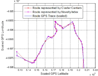
MIRGKL for Location Recognition Using GPS Stream Data ... 40

3.5.3

MIRGKL for Road Automatic Segmentation ... 46

3.5.4

Comparison between Original RGKL and MIRGKL with GPS Trip Data ... 48

3.5

C

N

S

... 49

CHAPTER 4: MACHINE AND SYSTEM PROGNOSTICS WITH EVOLVING

CLUSTERS EMBEDDED WITH LOCAL SURVIVAL FUNCTIONS ... 51

4.1

REMAININNG

USUFUL

LIFE

(RUL)

LEARNING

AND

ESITMIATION

USING

MIRGKL-

A

... 52

4.1.1

M

I

G

-K

-L

(MIRGKL)

C

A

MIRGKL-

... 52

4.1.2

W

S

F

A

L

A

F

... 53

4.2

EXPERIMENT:

DRILL-BIT

RUL

ESTIMATION ... 57

4.2.1

E

S

... 57

4.2.2

F

E

I

RUL

I

... 57

4.2.2.1 Dynamic Time Warping (DTW) Algorithm ... 57

4.2.2.2 Feature Extraction of Drill-bit Data with DTW ... 58

4.2.2.3 Determine Inferred RUL Information ... 60

4.2.3

RESULTS... 61

4.2.3.1 Initial Data Analysis ... 61

4.2.3.2 Setup #1 – Fully Online Mode (Perfect Information) ... 64

4.2.3.3 Setup #2 – Semi-Online Mode (Delayed Information) ... 67

4.3

BRAKE

WEAR

MONITORING

WITH

MIRGKL-PLUS

ALGORITHM ... 72

4.3.2 Feature Extraction ... 75

4.3.3 Normalized Remaining Useful Life ... 79

4.3.4 Results ... 83

4.5

CONCLUSION

AND

NEXT

STEPS ... 88

CHAPTER 5: DATA EVOLUTION BASED DIAGNOSTICS AND PROGNOSTICS

WITH EVOLVING CLUSTERS ... 90

5.1

DATA

EVOLUTION

BASED

DIAGNOSTICS

AND

PROGNOSTICS ... 91

5.1.1 Pattern of Cluster Creations and Cluster Health Quantification ... 91

5.1.2 Cluster Transitions and Change in Patterns of Transitions ... 93

5.1.3 Cluster Utilization, Homogeneity and Crispness of Boundaries ... 96

5.1.4 Novelty Detection at the Macro and Micro Level ... 99

5.2

CONCLUSION

AND

NEXT

STEPS ... 99

CHAPTER 6: PUBLICATIONS, CONCLUSIONS AND NEXT STEPS ... 101

6.1

PUBLICATIONS ... 101

6.2

CONCLUSION

AND

NEXT

STEPS ... 102

REFERENCES: ... 105

ABSTRACT ... 121

LIST OF FIGURES

Figure 1: Illustration of the concept of optimal maintenance with failure and maintenance costs

[F05] ... 9

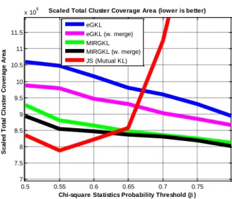
Figure 2: Total Coverage of Different Clustering Algorithms vs Proposed MIRGKL with

Merging Mechanism. ... 42

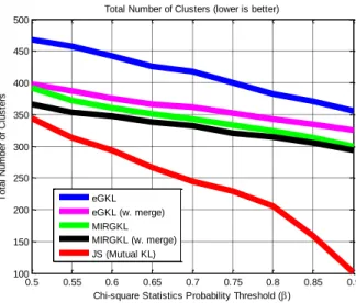
Figure 3: Total Number of Clusters Generated by Different Clustering Algorithms vs Proposed

MIRGKL with Merging Mechanism... 43

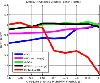
Figure 4: Entropy of the Centroids of Clusters Generated by Different Algorithms vs Proposed

MIRGKL with Merging Mechanism... 44

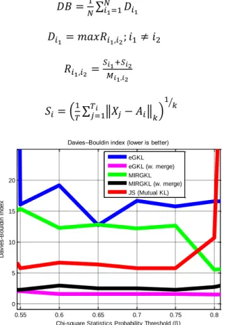
Figure 5: Davies-Bouldin Indices of the Centroids of Clusters Generated by Different

Algorithms vs Proposed MIRGKL with Merging Mechanism ... 45

Figure 6: Compress GPS Trace with Modified MIRGKL Online Clustering Algorithm ... 47

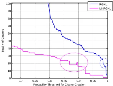
Figure 7: RGKL vs MIRGKL with different probability thresholds with GPS trip trace data .... 48

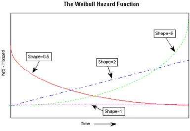
Figure 8: Weibull Hazard Function with different shape parameters ... 54

Figure 9: Feature calculation using Dynamic Time Warping (DTW) with Thrust Force (upper

figure) and Torque (lower figure) with multiple drill-bits. Blue lines represent drill-bits lasted

less than 30 drilling tasks and pink line represent those lasted more than 30 drilling tasks ... 59

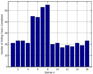
Figure 10: Number of drilling tasks completed for all 16 drill-bit in the experiment ... 62

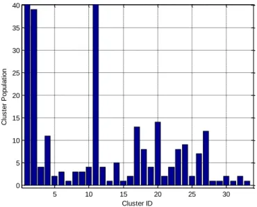
Figure 11: Population of each cluster identified by MIRGKL Algorithm ... 63

Figure 12: Normalized Inferred RUL vs Predicted RUL for Drill-bit #1~#4 ... 65

Figure 13: Normalized Inferred RUL vs Predicted RUL for Drill-bit #5~#8 ... 66

Figure 14: Normalized Inferred RUL vs Predicted RUL for Drill-bit #9~#16 ... 67

Figure 15: Normalized Inferred RUL vs Predicted RUL for Drill-bit #1~#4 in Delayed Online

Setup ... 68

Figure 16: Normalized Inferred RUL vs Predicted RUL for Drill-bit #5~#8 in Delayed Online

Setup ... 69

Figure 17: Normalized Inferred RUL vs Predicted RUL for Drill-bit #9~#16 in Delayed Online

Setup ... 70

Figure 18: Learned cluster specific degradation models of clusters with 3% (10 points) of all

data points ... 71

Figure 19: Learned cluster specific degradation models of clusters with 3% (10 points) of all

data points (Zoom-in View) ... 72

Figure 20: (upper) and Figure 4.15 (lower):

𝑋𝑑𝑒𝑐𝑒𝑙_𝑝𝑟𝑒𝑓

(upper) shows the deceleration

preferences and

𝑋𝑑𝑒𝑐𝑒𝑙_𝑒𝑓𝑓𝑖

(lower) shows a long-term performance of the braking system. .. 78

Figure 21 Example of timeline of events of data upload, clustering triggered by feature

calculated from cumulative statistics and interpolated inferred RUL. ... 80

Figure 22: Measured (Solid Dots) and inferred (Unfilled Circles) RUL of Front Driver’s Side

Brake Pad Thickness ... 81

Figure 23: Measured (Solid Dots) and inferred (Unfilled Circles) RUL of Front Driver’s Side

Brake Pad Thickness against Cumulative Braking Distance as the X-axis ... 82

Figure 24: Measured (Solid Dots) and inferred (Unfilled Circles) RUL of Front Driver’s Side

Brake Pad Thickness against Cumulative Braking Distance as the X-axis ... 83

Figure 25: Driver #1, Inferred Normalized Brake Wear (blue) vs Predicted Brake Wear. Top –

Bottom: Front Driver Side, Front Passenger Side, Rear Driver Side and Rear Passenger Side . 86

Figure 26: Driver #2, Inferred Normalized Brake Wear (blue) vs Predicted Brake Wear. Top –

Bottom: Front Driver Side, Front Passenger Side, Rear Driver Side and Rear Passenger Side . 87

Figure 27: Driver #3, Inferred Normalized Brake Wear (blue) vs Predicted Brake Wear. Top –

Bottom: Front Driver Side, Front Passenger Side, Rear Driver Side and Rear Passenger Side . 87

Figure 28: Driver #4, Inferred Normalized Brake Wear (blue) vs Predicted Brake Wear. Top –

Bottom: Front Driver Side, Front Passenger Side, Rear Driver Side and Rear Passenger Side . 88

Figure 29: Driver #5, Inferred Normalized Brake Wear (blue) vs Predicted Brake Wear. Top –

Bottom: Front Driver Side, Front Passenger Side, Rear Driver Side and Rear Passenger Side . 88

Figure 30: Differences between normal vs. cancer cells [VW15] ... 96

CHAPTER I INTRODUCTION

This chapter provides the motivation for the research and concludes with a statement of research. We start first with a brief introduction to common maintenance engineering practices before describing Condition-based Maintenance (CBM) and associated benefits. We also discuss the domain of evolving models and associated benefits. These sections form the foundation for discussing the specific research objectives at the end of the chapter.

1.1 CONDITION-BASED MAINTENANCE

Maintenance plays an important role to ensure the capacity of a system is being kept at a high level by keeping critical equipment and components’ overall availability, reliability and safety in check. Traditionally, maintenance activities can be classified into three categories, improvement maintenance (IM), preventive maintenance (PM) and corrective maintenance (CM) [Pat02]. IM aims at reducing the need of any maintenance activities in the design and operation phase of a system and as a result is highly cost prohibitive and impractical for most equipment or systems [Yan02]. CM deals with restoring a machine’s functionality after occurrence of failures. Often times, these failures cause line stoppage in production facilities and damage not only to the system itself but other systems as well. For certain equipment such as special purpose military vehicles or airplanes, any occurrence of a catastrophic failure is unacceptable due to potential loss of life and other losses.

Preventive maintenance focuses on activities that will prevent or minimize the occurrences of a failure. In turn, PM activities are considered effective when the levels of desired asset availability and reliability are high [Rao92]. Typical practices of PM are time or cumulative usage based where certain maintenance activities are prescribed as the asset reaches certain time or cumulative based milestone. Effectively, PM activities trade-off more frequent maintenance activities to unplanned (and at times catastrophic) failures that require CM. It improves total uptime by reducing downtime incurred by failures at the cost of some downtime associated with

PM activities. In PM, one of the most difficult decisions is related to the determination of the maintenance period. Since PM activities often involves change or recondition several components or subsystem, total time, labor and money invested in PM typically increases as maintenance period decreases. For example, if one were to employ the mean-time-between-failures (MTBF) as the maintenance period, one would expect half the assets to experience some type of a failure while the others will experience none. To reduce the number of expected failures, one can reduce the maintenance period albeit at a potentially higher overall cost of maintenance [LT97]. Figure 1 illustrates this trade-off of maintenance frequency vs. total cost.

Figure 1: Illustration of the concept of optimal maintenance with failure and maintenance costs [F05]

Alternative to PM or CM, one can also consider the concept of Condition-based Maintenance (CBM) or predictive maintenance [Yan02]. CBM focuses on monitoring the condition of the asset and warrants maintenance activities only if impending failures are predicted or some indicative signatures suggesting unacceptable level of performance deteriorations have been observed [BG01, OSL02].

Traditionally, diagnostics and prognostics functionalities are the foundation of such CBM practices. “CBM is a maintenance program that recommends maintenance decision based on the information collected through condition monitoring” [JL06]. While the extremely vast extant literature reports good success in developing highly effective diagnostic algorithms for certain

classes of components and equipment (such as bearings, pumps, and motors), leading to so called “point solutions,” most of these successes are based on decades of academic and industrial research involving characterization and modeling of equipment behavior through extensive, expensive and involved physics based modeling that requires in-depth knowledge of the system (e.g., physics driven models) [BMT99], [KR02a], [HZ09] and [LOS09]. It is understandable that such approaches are warranted in dealing with mission-critical systems (that might involve loss of life or incur large financial costs due to its malfunction or breakage). However, methods that are more cost-effective, produce accurate results and with ease of calibration yet mass-deployable are also desirable for various reasons. Mainly, they provide the means for cost effectively monitoring a wide-array of equipment and systems that are not considered to be non-mission-critical. When properly designed and implemented effectively, unnecessary maintenance activities and cost can be reduced through accurate diagnostics and prognostics information [JL06].

1.2 PROGNOSTICS

Equipment prognostics provide valuable insight into a meaningful future time or usage horizon regarding the status of the health and remaining useful life of a system. Most widely used definition of prognostics is to predict how much (usage) time is remaining before a failure occurs [JL06]. Alternatively, it can be also defined as to the probability that an asset will operate fault and failure free up to a meaningful future time [LM030], [SF03]. In turn, it provides opportunities for better planning and scheduling of both operation and maintenance activities with more informed decisions as to the contingency plan for affected sites, personnel and facilities and timely acquisition of maintenance parts and other necessary resources for maintenance activities.

Prognostics models often built upon diagnostics and it is the process of estimating the Remaining Useful Life (RUL) of a machine by predicting the progression of a diagnosed failure [F05]. Statistical methods such as autoregressive integrated moving average (ARIMA) models and Hidden Markov Models (HMM) [KT08], machine learning methods such as Artificial Neural

Networks (ANN), Support Vector Machines (SVM) and Relevance Vector Machines (RVM) and Monte Carlo methods such as Particle Filter (PF) have been studied as the engine for prognostics modeling purposes [ZL11]. Not to be confused with “mean time to failure” (MTTF) or life expectancy that has to do with “a population” of the same or at least similar machine or component’s “average operational life”, RUL is specifically defined as the time to the next failure for “one particular machine” or component being monitored [EGBH00].

Different from a diagnostics task that typically determines type and severity of a fault and whether the machine is “presently” in a known faulty state, carrying out a prognostics task is much more difficult in practice due to the need to forecast information into the future. Since the underlying degradation phenomenon is stochastic in nature, accuracy, precision and confidence of a model need to be considered. Accuracy is the measure of closeness between estimated and actual time of failure. Precision is the model’s ability to remain accurate as the time horizon increases. Confidence is the probability that the actual RUL falls within the estimated RUL interval. As a result, high accuracy, narrow precision and high confidence values are desirable [EGBH00], [F05].

In the aircraft industry, systems comprised of diagnostics and prognostics capabilities are commonly referred to as Integrated Vehicle Health Management (IVHM). Information generated from IVHM is highly desirable for not only OEMs but also for product maintenance and service providers [EJJ13]. There is a growing trend in the aviation industry of moving away from traditional “producer only” role to a more service oriented business model. Due to the effectiveness of IVHM based maintenance strategies, the demand has been substantial from the airplane operators to retrofit their legacy fleet (that do not come with necessary hardware) with OEM IVHM hardware to take advantage of the added benefits of IVHM based prognostics technologies.

1.3 EVOLVABLE MODELS

Real-world engineering and manufacturing problems come with high levels of complexity and complex underlying dynamics requiring sophisticated methods and tools for building intelligent systems (ISs) that can learn and adapt online [KS02]. These types of systems are capable of increasing structural complexity, perform model refinement and update its knowledge base through interaction with the environment with learning mechanism that may be supervisory or non-supervisory by design [AK98 and YM98]. Clustering analysis, a discipline related to data-mining (focus on knowledge discovery) and machine learning (focus on prediction & incremental learning), can form a building block for such systems. Recently, there has been a renewed focus on online clustering methods applied in various problem domains including image processing, classification and system identification. Classical clustering methods include Fuzzy C-Means (FCM) [BE84], K-Nearest Neighbor (KNN) [A92], Mountain Clustering [YF94] and its variant the Subtractive Clustering algorithm assume the availability of all data, operate in batch mode and create crisp or fuzzy spheroid shaped clusters. Online clustering methods have been proposed for performing clustering tasks dealing with streaming type of data [FG10, SR12, TK12, DS11, AM11] with single pass operations.

The Gustafson-Kessel (GK) algorithm characterizes each cluster with a centroid and a covariance matrix as an extension to the original Fuzzy C-mean clustering method [GK]. GK employs the inner product distance norm formally known as the Mahalanobis distance [MD], which is calculated from a positive definite symmetric matrix A:

𝑑_𝑖𝑘2 = ‖𝑥_𝑘− 𝑣_𝑖‖_𝑠2_{𝑖= (𝑥}

𝑘− 𝑣𝑖)𝑇𝐴𝑖(𝑥𝑘− 𝑣𝑖), the norm inducing matrix Ai is calculated from pi,

the cluster volume, and Fi, the fuzzy covariance matrix of the ith cluster and n is the dimensionality

of the space where clustering takes place:

𝐴_𝑖 = [𝑝_𝑖det (𝐹_𝑖)]1 𝑛⁄ _𝐹

By doing so, GK algorithm rids of the restrictions being imposed on other clustering methods by allowing the creation of ellipsoidal shaped clusters with varying orientations and sizes and is relatively insensitive to data measurement scales. Extended versions of GK capable to dealing with data streams with single pass operation have been proposed by [FG10, GF09, DS11, SR12]. In [AF04], online data clustering mechanism was applied to identify Takagi-Sugeno (TS) type models consist of If-Then rules as its knowledgebase. Evolving Takagi-Sugeno (ETS) model is capable of utilizing its evolvable multi-model structure and parameters to decompose a non-linear system into simpler ones. Effectively, for a complex problem the clustering procedure acts as a mean to partition the whole operational space into crisp (non-overlapping) or fuzzy (allowing some overlapping) into smaller sets while a local (cluster specific) model is responsible to capture the dynamics within the proximity of the corresponding cluster. Various applications including diagnostics and prognostics, motion tracking, non-linear system identification and controls have been discussed in literature [FCT10, LC13, IA12, MB15].

1.4 PROBLEM STATEMENT

The development of generic data-driven diagnostic and prognostic methods with evolvable structure and parameters will be the focus of this research. Specifically, system prognostics functionalities including degradation and RUL estimation will be the focal point and the main exemplary application. Built upon a mutual information based distance measure applied to the extended version of the Gustafson-Kessel-like (MIRGKL) algorithm, a new evolving clustering method with built-in pruning mechanism and embedded local models will be proposed and applied to problems of different natures.

Sensor selection, feature extraction, data fusion and physics based or historical data based analysis, while all important aspects of the development of a capable monitoring system, they are beyond the scope of this research. In addition, there is no strict assumption as to the underlying distribution of the data except for the assumption of Gaussian. In other words, the focus of the

research will be mainly on the evolving data driven model and less so on the derivation of physical model based information extraction and associated signal processing procedures.

The research will conclude with reports based on proposed MIRGKL applied to degradation monitoring (with local adaptive models) and data compression (without local adaptive models). Proposed models will be validated by real-world data collected under different experimental scenarios and goals. For process degradation and RUL estimation, we will specifically address issues when the degradation or RUL signal is available less frequently when compared to other information channels.

1.5 ORGANIZATION OF THE DISSERTATION

Existing literature on evolvable models and fault and degradation monitoring is reviewed in Chapter 2. In Chapter 3, proposed evolving clustering method, Mutual Information based Extended version of Gustafson-Kessel-like Clustering (MIRGKL) will be discussed with a validation on GPS data. Chapter 4 is dedicated to MIRGKL with evolvable local models and is validated with lab collected (drill bit) data and field collected (brake wear) data. Both of the datasets we studied are with limited observability in terms of system degradation requiring special treatment during model training (inference through normalization and interpolation). Chapter 5 is the final chapter where conclusions, comments and directions of future work will be given.

Evolving clustering methods have advantage to deal with stream type of data when compared to traditional clustering methods that requires all data to be available at the time of operation. Gustafson-Kessel algorithm uses Mahalanobis distance measure where orientation and size of a cluster becomes adaptable due to its clusters being defined as sets of centroids and covariance matrices. Jensen-Shannon (JS) divergence, a branch of the more generic Bregman divergence, is dependent on the choice of a convex function and can lead to different divergence and distance measures. Examples include the squared Euclidean distance (ED), Mahalanobis distance (MD) and the well-known Kullback–Leibler divergence (KL) just to name a few. The novelty in this part of the research presented in Chapter 3 is the use of the mutual information

formulation originated from JS to MD where the similarity or divergence between two distributions is measured as a weighted quantity obtained through the creation and use of a mixture of distributions obtained from known ones. In addition, a pruning mechanism is added as a way to regulate the growth of the overall structural complexity. Without any local model attached to each cluster, we demonstrate the proposed new clustering algorithm and benchmarked it against other variants of the GK algorithm utilizing real-world GPS data. This part of the work effectively utilized the proposed MIRGKL as an engine for data compression and favorable results are obtained.

In Chapter 4, MIRGKL is extended with cluster specific local models (MIRGKL-plus) and such a design is inspired by the pioneering work on online identification and incremental refinement of Takagi-Sugeno rule base [YF94, AF04 and L08]. General difficulties include not being able to handle non-stationary processes, requiring assumptions regarding underlying data disruptions, assumption of data independence and lack of online incremental changes to the modeling mechanism are common in equipment and system prognostics literature. In addition, costly and infrequent observations for RUL or degradation signal is often assumed to be a non-issue where in the real-world remains to be one of the most daunting obstacles during the development of a prognostics model. By design, proposed model’s supervisory and unsupervisory learning mechanisms are decoupled, and as a result, alleviates many of the difficulties mentioned above where degradation signal may come much less frequently when compared to other data channels. MIRGKL with local models will be validated with lab collected drill bit data with no degradation measurement available in this chapter. Novelty detection is a broader definition of the process monitoring problem, and hence, will be used frequently in this chapter. In Chapter 5, we will discuss novelty detection based on data evolution characterized by the evolving cluster process. We will summarize some notions discussed in our published papers and extend the framework with newly proposed concepts.

Conclusions, comments and directions of future work will be given in Chapter 6, which is the last chapter of the dissertation.

CHAPTER 2: LITERATURE REVIEW

This chapter discusses previous work on evolvable models including evolving clustering and equipment prognostics in sections 2.1 and 2.2, respectively.

2.1 EVOLVABLE MODELS

An evolvable model (EM) performs incremental construction of an increasingly more sophisticated model structure and adaptation of relevant parameters as part of a growing knowledge base. Different from most adaptive methodologies that only adapt model parameters without modification to the overall model structure, EM typically operates through an optional unsupervised data clustering algorithm where partitioning of the overall operational space is carried. A partition of the operational space may be represented in the form of centroid and influencing radius pairs that may take the form of cluster center (focal point) and radius (radius of influence of a local model) pairs, cluster centers with the same fixed radius or clusters and covariance pairs where each cluster’s size and orientation may differ. In the case where the partition is set to be fixed, it is equivalent of multiple local models being activated based on different inputs and only local models’ parameters will be evolving through interaction with data. This type of model is attractive in practice in following situations: 1) System is not yet or too costly and time consuming to be fully characterized. 2) System with multiple operating modes. 3) Systems dynamics will be non-stationary during its interaction with the environment and through its usage life. 4) Piece to piece variations of the same system will be significant due to natural variations in combination with the effects as described in 2 and 3. It should be noted that piece to piece variations may be caused not only by a production process but driven by the application’s intended use such as a software based personal digital assistant that need to adapt and learn from different users that will exhibit unique usage patterns and usage conditions.

The Takagi-Sugeno (TS) type fuzzy model is a powerful yet practical method for model and control of complex systems. It uses the notion of linearization in fuzzily defined regions in the state

space which effectively decomposes the original nonlinear model into multiple linear ones covered by fuzzy partitions [YF94]. The original fuzzy inference system makes embedding human or expert knowledge to the initial knowledge base possible; learning of TS model from data represents the idea of structure and parameter identification through: 1. Incremental adaptation of existing focal points and their parameters. 2. Addition of new focal points and associated rule bases and 3. The consolidation of focal points that are deemed too similar [AF04]. In [F01], the principle of evolving models is applied to a process control problem where a rule base of models (model bank) was proposed. The model bank learning algorithm initially started with randomly initialized clusters. When a normalized measure for the winning adaptive model meet the update criteria ‖𝜃𝑗(𝑡)−𝜃𝑘‖

‖𝜃𝑡‖ < 𝜀, t denotes time, k denotes an unique existing adaptive model and ε denotes

the threshold for the normalized similarity measure, the k’th model will be updated with current system observations; otherwise, a new adaptive model will be initialized because none of the existing adaptive models share enough similarity with the current system observables that warrants the assignment of current data to an existing and subsequent use it as evidence to adapt the model. While this method takes the “winner takes all” approach when it comes to model adaptation and utilization, control actions governed by a committee of (top) models utilize normalized similarities as weights is possible.

Another type of evolving system utilizes predetermined state space partitions or granulation where local models are subject to adaptation during its learning phase. In the estimation or prediction phase, various granulation approaches (crisp or fuzzy) may be applied to further generalize the performance of the model where multiple local models may have their outputs taken into account in the final prediction. Markov models can be applied for control purposes where forecasting mechanism include projection of future states and use of corresponding local adaptive models. In [FT11], the state space is spanned by time of day and day of the week with local adaptive Markov model for driver destination predictions. The granulation of the state space

was designed to capture prototypical decision models in terms of location transitions. It should be note that different encoding methods such as fuzzy encoding may be applicable to not only generalize, smooth out model outcome it is beneficial to adopt such information granulation mechanism to overcome lack of training of certain local models in the initial phase of deployment of the model. Since the underlying learning mechanism is equivalent of imposing a moving window with a set of recursive procedures, the outcome is a “LIVING” database that contextually matches the user’s recent decisions for location transitions. Another aspect of applying information encoding with multiple local models is the improved consistency, usability and predictability of the outcomes of the model which is a crucial aspect for the design of systems that will have certain level of interactions with human.

Except for the case when the space granulation or partitioning has been pre-determined, at the center of an evolving model is typically to some extent a clustering method [MG14, LL01, ZD14]. The reason being that the design of the mechanism the enables self-adaptation shall be effective in its predictive performance yet sufficiently compact in its overall structural complexity is essentially the same task a clustering method performs.

2.1.1. Evolving Clustering

Clustering, synonymous to cluster analysis, classification, numerical taxonomy and typological analysis represents the task of grouping object (with descriptive data) such that object in the same group share more similarity when compared to objects in other groups [XW05]. Any clustering method is either supervised or unsupervised depending on the availability of the truth labels that consist of finite number of discrete assignable classes given some inputs [B95]. Most well-known clustering methods include Fuzzy C-Means (FCM) [BE84], K-Nearest Neighbor (KNN) [A92], Mountain Clustering [YF94], Support Vector Machine (SVM) [CV95] and Relevance Vector Machine (RVM) [T01]. Most clustering algorithms assume the availability of all data, operate in batch mode and create crisp or fuzzy spheroid shaped clusters. They have been applied in extensively in exploratory data mining and visualization, object detection, novelty detection,

knowledge discovery and acquisition, statistical data analysis, machine learning, pattern recognition and data representation and compression.

Online clustering methods have been proposed in [FG10, SR12, TK12, TS11, and AM11] with single pass operations where proposed models are evolvable both structurally and parametrically. Compared with batch type methods, they are specifically suitable for problems with following characteristics:

A. Stream Type of Data and Very Large Data (VLD): Mining and extraction of knowledge from existing dataset that is extremely large and cumulative data streams that, over time, grows significantly in its sheer size poses great challenging to most data modeling methods [GZ09]. For example, the number searches Google performs increased from 60 million during 2000 to 5.7 billion during 2014 on a daily basis. In modern vehicles, there are thousands of signals in its CAN (controller area network) updated at a speed at milliseconds. Even with down sampling, the amount of data grows very rapidly not only for storage but also for the identification of applicable means to analyze them. Tackling the task of modeling and extracting useful information from stream type of data or extremely large data requires a fundamental shift in the frame of mind of data miners as well as development of methodologies to be more applicable in these situations [DH01].

B. Dynamic Operating Conditions: A common challenge for real-life applications of clustering algorithm has to be with non-stationary data. Facial and voice recognition, metabolic pathways in biological cells, object tracking in computation vision and monitoring of equipment operating under distinct modes under the influence of random noises are just few examples [LA14, FC04a and FC04b]. Clustering methods operate in batch mode, assuming all data to be observable during structure and parameter identification phase, often requires the model to be re-trained if certain limits on the range input space have been exceeded rendering existing model to be invalid or facing

the risk of significantly degraded performance. On the other hand, evolvable clustering method are designed to take into account such conditions by evaluate the degree of deviation at both the overall model level as well as individual cluster level. Dependent on the level of deviation, either incremental adjustment can be made to existing clusters or a new cluster will be created to specifically account for new and emerging patterns. C. Uncertainty in Acquired Information: The ability to make subtle adjustment to existing

clusters to deal with signals embedded with varying level of drifts imposed by either the physical attributes of the underlying sensing hardware (i.e. GPS signals) along with varying noises types and impacts they have on the fidelity of the signal when interacting with the environment [FT11]. In some applications, this involves piece to piece variations as well as similarly purposed equipment equipped with different classes of sensors due to hardware advancement and for the purpose of differentiation in their portfolio accommodating different target industries and customers.

D. Building of Intelligent Systems: An intelligent system improves system performance through learning while preserving useful previously gained experience. It is a highly interdisciplinary field involves control theory, artificial and computational intelligence, biologically and life science inspired systems and various engineering disciplines [A12 and A13]. These systems rely on statistical and data driven mechanisms to adapt their flexible yet evolvable model structure and parameters temporally to accommodate both abrupt and slow changing dynamics [L08 and L15]. At their cores, these algorithms represent the development of goal-oriented self-learning machines engaging in extraction of new knowledge and conduct evidence based refinement to existing ones when opportunities present themselves.

Participatory learning (PL), based on unsupervised learning, provides a mean to identify structures of a rule-based system. It enables the learning process through compatibility evaluations between currently known belief and observations made in the learning environment

[R90]. Naturally, several unsupervised dynamic clustering algorithms have been proposed as part of a wave of adaptive systems [LG06, AF05 and OL04]. The original Evolving Takagi-Sugeno (ETS) model and its modified version Simpl_eTS model combine the supervisory and unsupervisory learning to dynamically identify new rule bases and modify existing ones. The unsupervisory part of learning mainly addressed the core issue of dividing the state space into sub-partitions (through recursive clustering) and the supervisory learning procedure establishes a local linear model for each sub-partition (cluster specific) [AF04 and AF05] for approximations of an overall non-linear system’s behavior.

One critical element in any clustering method is the distance (similarity) measure employed to determine: 1) Similarity between a new data to existing clusters for data assignment and cluster update purposes and 2) Similarity between existing clusters to evaluate the necessity of structure pruning. In addition, the choice of the distance measure will have a direct relationship as to how each identified cluster will be characterized and subsequent procedures for adaptation according to new evidence [AG01, BB91, CG91, HB00, M67, FT11 and MJ94]. The Mahalanobis distance is an unit-less and scale invariant distance measure generalized for the multi-dimensional space and enables the creation of ellipsoidal shaped clusters with variable orientation and sizes [M36].

𝐷𝑀(𝑋) = √(𝑥 − 𝜇)𝑇𝑆−1(𝑥 − 𝜇) (2) x: data point to be evaluated

u: cluster specific mean vector S: cluster specific covariance matrix

The recursive procedures to identify clusters using the Mahalanobis distance is presented in [FT11] where cluster specific local models were trained in a least square fashion and the evolution of the clustering process is tracked as serve as indicators for incipient and abrupt failures of a machine.

2.1.1. Gustafson-Kessel Clustering Algorithm and Bregman Divergence

The Gustafson-Kessel (GK) algorithm characterizes each cluster with a centroid and a covariance matrix and employs the inner product distance norm formally known as the Mahalanobis distance [MD] which is calculated from a positive definite symmetric matrix A:

𝑑_𝑖𝑘2 = ‖𝑥𝑘− 𝑣𝑖‖𝑠2𝑖= (𝑥𝑘− 𝑣𝑖)𝑇𝐴𝑖(𝑥𝑘− 𝑣𝑖), the norm inducing matrix Ai is calculated from pi,

the cluster volume, and Fi, the fuzzy covariance matrix of the ith cluster and n is the dimensionality

of the space in which the clustering procedure takes place:

𝐴𝑖 = [𝑝𝑖det (𝐹𝑖)]1 𝑛⁄ 𝐹𝑖−1

Extended version of GK capable to dealing with data streams with single pass operation has been proposed by [FG10, GF09, DS11, SR12]. It is worth to note that the single pass operation proposed in these methods, in contrast of iterative batch procedures, represents significant improvement in computational resources and memory requirement when dealing with very large or stream type of data where the size of the whole dataset may be undefined initially.

Bregman divergence [B67] represents divergences generated from some convex function. Examples include well-known Euclidean distance, Itakura-Saito distance, Kullbak-Leibler (KL) divergence and the Mahalanobis distance [BM05b]. A few examples of convex function of choice Ф(X) and corresponding distance measure dФ(X,Y) derived from definition of Bregman divergence are shown in Table 1 as follows:

Table 1:Bregman divergences generated from convex functions [BM05b]

Ф(X) dФ(X,Y) Divergence

x2 _(x-y)2 _{Squared loss}

-logx x/y-log(x/y)-1 Itakura-Saito distance ||x||2 _||x-y||2 _{Squared Euclidean distance} xT_{Ax (x-y)}T_{A(x-y) Mahalanobis distance}

∑ 𝑥_𝑗𝑙𝑜𝑔₂ 𝑑 𝑗=1 𝑥_𝑗 ∑ 𝑥_𝑗𝑙𝑜𝑔₂(𝑥𝑗 𝑦_𝑗) 𝑑 𝑗=1 Kullbak-Leibler (KL) divergence

It was shown in [BM05a] that clustering problems can be solved using Kmeans type of iterative schemes [HW79 and WC01] only if the underlying distortion applied as a distance measure is from the family of Bregman divergence. Furthermore, it was also proven that the minimization between data points to identified cluster centroids is equivalent to the loss in Bregman information therefore the minimizing either produced the same optimal clustering result [BM05b]. Jenson-Shannon divergence (JSD), a variant of KL divergence provides an inspiring formulation that is applicable to other Bregman family of divergences that yields a smoothed, symmetrized and bounded form when compared to its original forms [L91].

2.2 EQUIPMENT PROGNOSTICS

Diagnostics tasks are defined as the ability to detect, localize and determine the severity of a fault in a system that is “currently” in a failure state; prognostics tasks are often much more difficult to be carried out in practice because the need to perform forecasting into the future. As a result, it is often referred to as the Achilles’ heel of CBM systems. Prognostics research historically has much less available literature when compared to diagnostics methods [VWK99] due to difficulties surrounding elements to be forecasted are relevant to a stochastic process and specifically the availability of usable features and enabling techniques to support such development of prognostics functionalities could be difficult to obtain [BM99]. So far, center of the attention of such efforts often focus on systems with slow and progressive degradations pattern leading to eventual failure including mechanical and structural systems [Mar01]. While prognostics often built upon diagnostics functionalities, it has a stronger emphasis on predicting the Remaining Useful Life (RUL) [WC01] and the progression of a diagnosable failure [F05] through prognosis assessment. In the literature, statistical methods (i.e. Autoregressive Moving Average or ARMA model), stochastic methods (i.e. Hidden Markov Model or HMM) [KT08] and

machine learning methods (i.e. Artificial Neural Network or ANN, Support Vector Machines (SVM) and Relevance Vector Machines (RVM)) [WC01, CW10 and HL07] all have been applied as means to perform prognostics tasks. One should not confuse the RUL estimation with the notion of “Mean Time to Failure” (MTTF), the prior (RUL) has to do with a specific machine or system’s predicted remaining life with respect to time or other cumulative usage unit while the latter is more relevant to a “population wise” attribute in an average sense [EGBH00].

Aside from data-driven methods mentioned in the previous paragraph, physics or model-based methods have been developed for various types of equipment with much success. However, these types of efforts are mostly reserved for mission critical systems and equipment due to extensive efforts and dedicated experiments required to establish the model [BM99, KRM02]. Application of the same model to similarly purposed, updated equipment with design differences or equipment under completely different usage patterns in most cases are not feasible. In those cases, development and calibration procedure typically need to be repeated to be able to achieve good performance in the field [RK00, TV01 and HH01]. In recent Condition Based Monitoring (CBM) literature, data-driven prognostics started to utilize methods developed for survival analysis and specifically the reliability function such as Weibull distribution [GH09].

2.1.1. Data-Driven Methods for Prognostics

Traditional reliability models such as Weibull, Poisson and Log-Normal distribution based estimation methods characterizes population performance degradation patterns to enable longer-term forecast of RUL [SR03 and G00]. However, this type of model often provides predicted RUL information not accurate enough for individual units [HZ09]. As a result, Machine Learning (ML) based method and hybrid models utilizing ML techniques have been proposed in [CC10, FT08, B14, J07, JR06, SG09, DT12 and NA14] that can deal with stochastic degradation signatures and operation environment, make few to no assumption as the underlying signal distributions yet integratable with physical understanding of a system and some of them with online adaptable model structures and parameters [FT06a and FT06b]. In [CC05 and KT08], Hidden Markov Model

applied through utilizing a hierarchical structure and as a mean for sequential clustering for the purpose of drill bit health diagnostics. Though RUL information was not explicitly expressed, they indirectly obtained equipment RUL information in the form of cumulative equipment usage as total number of tasks conducted so far through knowledge of each drill bit started to be brand new and End of Life (EOL) was reached until each of them can no longer carry out the prescribed drilling tasks. They represent a case where indirect inference of RUL information can be inferred for the purpose of diagnostic model but could also be applicable for the development of prognostics models.

2.1.2. Usage of Prognostics based Information

In contrary to the vehicle industry, the aircraft and military industry have been moving at a much faster pace to apply Integrate Vehicle Health Maintenance systems (IVHM) or Prognostics and Health Management (PHM) system to fully utilize diagnostics and prognostics information produced by such systems. To move away from the of being sole manufacturers, IVHM has become highly desirable as a way for OEM’s to enhance maintenance programs, improve logistics efficiency and being able to offer services at a more customized level to their customers[EJJ13]. Due to the effectiveness of IVHM based maintenance strategies, the demand has been substantial from the airplane operators to retrofit their legacy fleet (that do not come with necessary hardware) with OEM IVHM hardware to take advantage of the added benefits of advanced diagnostics and prognostics technologies. With various industries’ renewed focus on reducing downtime and critical failures [KT06], maintaining system’s operational safety and ongoing maintainability [SZ10] and to able to address reliability issues arise from more complex design and ever more demanding operation conditions during lifecycle of a produce, PHM and IVHM systems with integrated prognostics functions will play a crucial role in effective fulfillment of Produce-service system (PSS) contracts [DA11 and LT12]

CHAPTER 3: MUTUAL INFORMATION BASED RECURSIVE

GUSTAFSON-KESSEL-LIKE CLUSTERING ALGORITHM (MIRGKL)

The notion of a “cluster” cannot be precisely because its meaning and property varies depending on the applications or algorithms [E02]. Nevertheless, clustering is generally synonymous to cluster analysis, classification, numerical taxonomy and typological analysis and represents the task of grouping object (with descriptive data) in a manner such that object in the same group share more similarity when compared to objects in other groups [Jain 1999 and XW05]. Different from classification, which is typically a supervised task where some predefined labels consist of finite number of distinct classes is available; clustering is mostly an unsupervised task where there exists no true label for each piece of information. Over the years, methods include Fuzzy C-Means (FCM) [BE84], K-Nearest Neighbor (KNN) [A92], Mountain Clustering [YF94] and their early variants operate in batch mode and create crisp or fuzzy spheroid shaped clusters with some predefined parameters including cluster radius or number of clusters to be identified. Originally proposed and applied for anthropology [DK32] and psychology [T39] research, clustering algorithms been applied extensively in exploratory data mining and visualization, object detection, novelty detection, knowledge discovery and acquisition, statistical data analysis, machine learning, pattern recognition and data representation and compression.

Online clustering methods have been proposed for performing the same clustering tasks dealing with stream type of data or very large data (VLD) [FG10, SR12, TK12, TS11, AM11] with single pass operations. These online evolvable clustering algorithms allow incremental changes to be made both structurally and parametrically through respective data-driven mechanisms. More recently, online clustering methods have been heavily researched and applications in objective detection, diagnostics and prognostics and system identification due to their much improved capability through embedded adaptable model or function specific to each identified cluster [AF10]. In [L08], development has been made where prediction performance of such model is comparable to a physics based model for a rather complex system.

Gustafson-Kessel (GK) clustering characterizes a cluster with a centroid and a covariance matrix and represents a major improvement over traditional methods with its ability to better adapt to real-world data that comes in different shapes and forms [GK78]. The distance measure GK employs what is formally known as the Mahalanobis distance. Alternatively, it can be expressed as the following:

𝑑_𝑖𝑘2 = ‖𝑥𝑘− 𝑣𝑖‖𝑠2𝑖= (𝑥𝑘− 𝑣𝑖)𝑇𝐴𝑖(𝑥𝑘− 𝑣𝑖) (3)

The norm inducing matrix Ai is calculated from pi, the cluster volume, and Fi, the fuzzy

covariance matrix of the ith cluster and n is the dimensionality of the space in which the clustering procedure takes place:

𝐴𝑖 = [𝑝𝑖det (𝐹𝑖)]1 𝑛⁄ 𝐹𝑖−1

It has been shown in that clustering problems can be solved using K-means type of iterative schemes [HW79 and WC01] only if the underlying distances measure are from the family of Bregman divergence [BM05a]. Furthermore, it was also proven that the minimization between data points to identified cluster centroids is equivalent to the loss in Bregman information therefore the minimizing either produced the same optimal clustering result [BM05b]. Bregman divergence [B67] represents divergences generated from some convex functions and examples include well-known Euclidean distance, Itakura-Saito distance, Kullback-Leibler (KL) divergence and the Mahalanobis distance [BM05b]. Jenson-Shannon divergence (JSD), a variant of KL divergence provides an inspiring formulation that is applicable to other Bregman family of divergences that yields a smoothed, symmetrized and bounded properties when compared to its originating divergence the KL divergence [L91].

Extended version of GK operates recursively (single pass operation) has been proposed by [FG10, GF09, DS11, SR12]. Single pass operation proposed in these methods, in contrast of iterative batch procedures, represents significant improvement in the reduction of computational resources and memory requirement. Similar to other online clustering methods such as [QW08,

TK12, BL05, BZ06 and AF04] they are designed to deal with very large data (VLD) or stream type of data where the size of the whole dataset may be very large or initially undefined. Online clustering methods are critical in the development of intelligent systems that are goal-oriented self-learning machines engaging in extraction of new knowledge and conduct evidence based refinement to existing ones when opportunities present themselves [KS02, A12 and A13].

This article proposes a novel Mutual Information based Recursive Gustafson-Kessel Clustering Algorithm (MIRGK). We will briefly describe the original version of the extended Gustafson-Kessel algorithm in section 2, describe in detail the proposed mutual information based version in section 3, Experiment and validation using real-world GPS data will be given in section 4, and finally we will conclude the paper with summary and future work in section 5.

3.1 EXTENDED VERSION OF THE GUSTAFSON-KESSEL (GK) ALGORITHM

In real-life applications, we are often encountered with data exhibiting varying non-stationary behaviors, generated from noisy operating conditions and tend to grow in its amount as usage being accrued [SR12]. While it is not uncommon to restart the clustering algorithm by using only a fraction of data, it is not a very efficient way of carrying out such task and by doing so also defeat the purpose of the intention of extracting useful information from all the data. As a result, online clustering is of particular interest recently in fields such as pattern recognition, machine learning and non-linear system identification [DH12]. The extended version of Gustafson-Kessel algorithm [FG10 and DS11] operates recursively to update cluster specific parameters including the centroid, the inverse covariance matrix and the determinant of the original covariance matrix. In [FG10], a detailed and more generic version of the updating procedure based on Exponentially Weighted Moving Average (EWMA) was derived:

𝑉_𝑖,𝑡 = (1 − 𝛼) ∗ 𝑉_{𝑖,𝑡−1}+ 𝛼 ∗ 𝑋_𝑡 = 𝑉_𝑖,𝑡+ (1 − 𝛼) ∗ (𝑋_𝑡− 𝑉_{𝑖,𝑡−1}) (4)

𝐹_𝑖,𝑡−1= (𝐼 − 𝐺_𝑖∗ (𝑋_𝑡− 𝑉_{𝑖,𝑡−1})) ∗ 𝐹_{𝑖,𝑡−1}−1 ∗_1−𝛼1 (5) where

𝐺_𝑖 = 𝐹_{𝑖,𝑡−1}−1 _{∗ (𝑋}

𝑡− 𝑉𝑖,𝑡−1)𝑇∗_{1−𝛼+𝛼∗(𝑋} 𝛼

𝑡−𝑉𝑖,𝑡−1)∗𝐹𝑖,𝑡−1−1 ∗(𝑋𝑡−𝑉𝑖,𝑡−1)𝑇 (6)

𝑑𝑒𝑡𝐹𝑖,𝑡= (1 − 𝛼)𝑛−1∗ 𝐹𝑖,𝑡−1∗ (1 − 𝛼 + 𝛼 ∗ (𝑋𝑡− 𝑉𝑖,𝑡−1) ∗ 𝐹𝑖,𝑡−1−1 ∗ (𝑋𝑡− 𝑉𝑖,𝑡−1)𝑇) (7) It should be noted that i denotes the i’th cluster, t denotes time instant, V, F and detF are cluster specific centroid, covariance matrix and determinant of the covariance matrix. The procedure employs Sherman-Morrison-Woodbury or simply Woodbury formula [W50] to derive the recursion of the inverse covariance matrix. Additional cluster specific credibility value M increments whenever a data falls into the coverage of a cluster. This parameter functions as a relaxation mechanism in the cluster algorithm’s data assignment and cluster update procedure. Effectively, this allows additional incremental adjustment to clusters that have been receiving little evidence for subsequent refinement since creation and increase the coverage of all available space occupied by all clusters to be maximized. [FG10] also suggested the use of negative updates to non-receiving clusters to mitigate issues with overlapping clusters common in GK derived clustering algorithms.

The application of (4-7) supports at least 3 flavors of online versions of GK derived clustering algorithms including the recursive evolving version GK(eGK), evolving GK-Like (eGKL) algorithm [FG10]. While the main elements are quite similar in notion, eGK and eGKL algorithm are different in a few key steps. First of all, eGKL may start from scratch with either some clusters already been identified (either from a initialization step or from the previous execution) while eGK relies on the existence of some clusters. In addition, the credibility of an existing cluster in eGK is estimated at each step to determine enclosure of points while in eGKL this is done through increment a cluster specific value in the data assignment process as a result a more relaxed and computationally less taxing procedure. While sharing the same updating procedure of the winning cluster (4-7), eGKL performs an additional update to the centroids of non-winning clusters adopting a negative learning rate to move them slightly away from the current data. Lastly, the distance or similarity measure in eGK is the original Gutafson-Kessel formulation where the norm

induction includes a fuzzification term det(F)1/n_{; while in the eGKL the provision was made to have}

the flexibility of choosing between some unit-less measures including the Gustafson-Kessel norm inducing formulation or the Mahalanobis distance. The main steps of eGK and eGKL clustering algorithms are organized side by side and summarize the following table.

Table 2: Comparison of Key Steps in eGK v.s. eGKL Clustering Algorithm Clustering Steps Evolving GK Algorithm Evolving GK-Like Algorithm 1. Initialization Batch GK or other clustering algorithms Optional; may start from scratch 2. Distance / Similarity Measure 𝑑𝑖,𝑘= √(𝑋𝑘− 𝑉𝑖)[(det(𝐹𝑖))1/𝑛𝐹𝑖−1](𝑋𝑘− 𝑉𝑖)𝑇 𝐷𝑖,𝑘 2 _{= (𝑋} 𝑘− 𝑉𝑖)𝐹𝑖−1(𝑋𝑘− 𝑉𝑖)𝑇 or 𝑑𝑖,𝑘 3. Cluster Assignment Criteria dp,k ≤ rp 𝐷𝑝,𝑘2 < 𝒳𝑛,𝛽2 𝑜𝑟 𝑀𝑝< 𝑀𝑚𝑖𝑛 4. Winning Cluster Updates (4 - 7) (4 – 7) 5. Non-Winning Cluster Update

N/A Centroids moving away from sample with a

negative learning rate

Evidential evolving GK (E2GK) [SR12] was inspired by eGK and Evidential Fuzzy C-means Algorithm (ECM) [MD08]. In [SR12], E2GK creates credal partitions (similar in concept to fuzzy but more genera) using belief function theory and adopts the same cluster adaptations using (4 - 7).

3.2 Mutual Information based Recursive Gustafson-Kessel Clustering Algorithm

Post cluster assignment, eGK and eGKL maintain cluster credibility parameters that are calculated differently but both serve as a mean to control the total number of clusters being created. In eGK, such parameter for a new cluster is assessed to determine if a meaningful amount of number of existing data points are within its coverage. Failure to meet such criteria results in removal of the newly added cluster and the overall cluster reverted to the one prior to processing the current data point. On the other hand, in eGKL the credibility parameter provides opportunistic additional updates to clusters that are not yet considered to be well defined. It is

worth noting in eGKL the provision of having “infant” or “emerging” stage clusters’ absorption of new data fall into a proximity region reduces the propensity in eGK where non-consecutive yet similar patterns may not be properly captured.

The structure complexity regulation mechanisms described above focus on evaluation of new or relative new clusters’ coverage to known data points by calculations of cluster specific credibility scores. Another avenue to ensure conditions led to creation of a new cluster is truly warranted is study the more fundamental aspects of a clustering algorithm which is the similarity measure of choice.

3.2.1 Mutual Information based Mahalanobis Distance

In [D07], the well-known Kullback-Leibler (KL) divergence for two distributions ℵ₀ and ℵ₁with mean,µ0 and µ1, and covariance matrices, ∑0and ∑1, of the same dimension is expressed in the following matrix form:

𝐷𝐾𝐿(ℵ0||ℵ1) =1₂(𝑡𝑟(∑1−1∑0) + (µ1− µ0)𝑇∑1−1(µ1− µ0) − 𝑘 + ln (𝑑𝑒𝑡∑_{𝑑𝑒𝑡∑}1

0)) (8)

The terms calculating the trace of the ratio between ∑₀and ∑₁ and the natural log of the ratio between the determinant of ∑₀and ∑₁ are related to the comparison of the size and shape of the distributions as defined in their respective covariance matrices. The remaining terms include the dimensionality expressed in k and (µ₁− µ₀)𝑇∑₁−1(µ₁− µ₀) which is nothing but the original definition of the Mahalanobis Distance [M36]. As a result, one can consider the Mahalanobis distance as a special case for the more generic definition as defined by the KL-divergence.

Bregman divergence represents a more generic divergences generated from some convex functions [B67]. It was shown in [BM05a] that clustering problems can be solved using K-means type of iterative schemes [HW79 and WC01] only if the underlying distortion applied as a distance measure is from the family of Bregman divergence. Examples of divergences derived from the Bregman divergence, not surprisingly, include well-known Euclidean distance, Itakura-Saito

distance, Kullback-Leibler (KL) divergence and the Mahalanobis distance [BM05b]. A few examples of convex function of choice Ф(X) and corresponding distance measure dФ(X, Y) derived from definition of Bregman divergence are shown in Table 1 as follows:

Table 3: Bregman divergences generated from convex functions [BM05b]

Ф(X) dФ(X,Y) Divergence

x2 _(x-y)2 _{Squared loss}

-logx x/y-log(x/y)-1 Itakura-Saito distance ||x||2 _||x-y||2 _{Squared Euclidean distance} xT_{Ax (x-y)}T_{A(x-y) Mahalanobis distance}

∑ 𝑥𝑗𝑙𝑜𝑔2 𝑑 𝑗=1 𝑥𝑗 ∑ 𝑥𝑗𝑙𝑜𝑔2( 𝑥_𝑗 𝑦𝑗) 𝑑 𝑗=1 Kullbak-Leibler (KL) divergence

Furthermore, it was also proven that the minimization between data points to identified cluster centroids is equivalent to the loss in Bregman information therefore the minimizing either produced the same optimal clustering result [BM05b]. Jenson-Shannon divergence (JSD), a variant of KL-divergence provides an inspiring formulation that is applicable to other Bregman family of divergences that yields a smoothed, symmetrized and bounded form when compared to its original forms [L91] defined as the following:

𝐷_𝐽𝑆(ℵ₀||ℵ₁) =1₂𝐷_𝐾𝐿(ℵ₀||ℵ_𝑀) +1₂𝐷_𝐾𝐿(ℵ₁||ℵ_𝑀) (9)

Where ℵ_𝑀= 1 2ℵ0+

1 2ℵ1

The Jensen-Shannon divergence is the mutual information between a random variable to a mixture distribution NM between the two distributions of interest, namely N0 and N1. DKL as shown in (9) represents the KL-divergence value between two distributions and DKL(N0||N1) is different from DKL(N1||N0). A special case for (9) where the shape and size information contained in the

covariance matrix not to be taken into account separately other than as a normalizer would become the following:

𝐷𝑀𝑀(ℵ0||ℵ1) =1₂𝐷𝑀(ℵ0||ℵ𝑀) +1₂𝐷𝑀(ℵ1||ℵ𝑀) (10)

Where ℵ_𝑀= 1₂ℵ₀+1₂ℵ₁

And DM is the original Mahalanobis Distance:

𝐷_𝑀(ℵ₀||ℵ_𝑀) = √(µ0− µ𝑀)𝑇∑𝑀−1(µ0− µ𝑀) (11) In essence, the formulation presented by the Johan Jensen and Claude Shannon as shown in [L91] applied the original KL-divergence calculations from the perspective of a mixture distribution denoted by NM against the two distributions of interest, N0 and N1. As a result, the KL-divergence with the Jensen-Shannon formulation can be understood as the weighted average of Ni with respect to NM where Ni are the distributions that their difference need to be quantifiably measured and NM is a linear combination of Ni. The fact that the Jensen-Shannon formulation transformed the originally unbounded KL-divergence to be bounded and symmetrized the originally asymmetric similarity measure brings in significant improvement in numerical stability when utilizing such measures. Since (11) is simply partial formulation of the original (8), such property will be useful when applied in a clustering algorithm to subdue the likelihood of creation of new clusters and stabilize the cluster assignment process simultaneously.

3.2.2 Threshold Setting in Cluster Assignment, New Cluster Creation and Merging

In [FG10, FT06a and FT06b], the similarity measure of the most similar (or winning) cluster to the current data is subjected to a threshold to determine if the level of closeness warrants the assignment (of the current to the winning cluster) and subsequent updates made to its parameters:

𝐷2_{< 𝒳}

𝑛,𝛽2 (12) This is based on the interpretation of the Mahalanobis distance as the summation of the squares of random variable where n denotes the number of random variables involved (or

dimensionality) and β is the threshold associated with a probability value. Given a problem need to be tackled by a clustering algorithm, the value of n is typically fixed and the choice of β controls the propensity of new cluster creation and the total number of clusters to be obtained. The reason for this is quite straight forward because a higher value of β will result in a larger value of 𝒳_𝑛,𝛽2 as it represents that for this particular cluster the likelihood of seeing the similarity measure exceeding 𝒳_𝑛,𝛽2 will be (1-β). In other words, the higher β (therefore a higher value of 𝒳_𝑛,𝛽2 ) given that dimensionality and the definition of similarity are fixed, the radius of influence of the same cluster will be increased and eventually lead to the final resulting number of clusters to be lower to represents the same set data. While we modified the similarity measure in the original eGKL to (10, 11), the Kohonen rule [K12] to update the winning cluster. When any assignment is not possible, a new cluster will be created with a default covariance matrix.

The evaluation of the merging existing clusters focusses on (C-1) pairs of clusters consists of the current active cluster and one of the remainder of the clusters where C denotes the total number of clusters. The merging of a pair of clusters, each represents different set of data points and is a result of incremental refinement based on these points, involves the combination of their respective parameters and shall be treated with more caution. Due to this reason, we propose to use (Ch-2 1) but with a different β denoted as βM where M represents merging:

𝐷_𝑀2 _{< 𝒳} 𝑛,𝛽𝑀

2 ₍₁₃₎ The parameter βM, specifically for the purpose of cluster merging, shall be a number smaller than the original β which is specifically for cluster assignment. This treatment in the evaluation of merging a pair of clusters represents a more restrictive and conservative approach as to combining two existing clusters. Another way to understand that βM should be strictly smaller than β is as this parameter decreases; it is equivalent of imposing a tighter control limit during similarity evaluation. In other words, a random variable meeting the threshold established