Towards a multipurpose neural network approach to novelty detection

a thesis submitted to The University of Kent in the subject of computer science

for the degree of doctor of philosophy.

By Simon J. Haggett

Novelty detection, the identification of data that is unusual or different in some way, is relevant in a wide number of real-world scenarios, ranging from identifying unusual weather conditions to detecting evidence of damage in mechanical systems. However, utilising novelty detection approaches in a particular scenario presents significant challenges to the non-expert user. They must first select an appropriate approach from the novelty detection literature for their scenario. Then, suitable values must be determined for any parameters of the chosen approach. These challenges are at best time consuming and at worst prohibitively difficult for the user. Worse still, if no suitable approach can be found from the literature, then the user is left with the impossible task of designing a novelty detector themselves.

In order to make novelty detection more accessible, an approach is required which does not pose the above challenges. This thesis presents such an approach, which aims to automatically construct novelty detectors for specific applications. The approach combines a neural network model, recently proposed to explain a phenomenon observed in the neural pathways of the retina, with an evolutionary algorithm that is capable of simultaneously evolving the structure and weights of a neural network in order to optimise its performance in a particular task.

The proposed approach was evaluated over a number of very different novelty detection tasks. It was found that, in each task, the approach successfully evolved novelty detectors which outperformed a number of existing techniques from the literature. A number of drawbacks with the approach were also identified, and suggestions were given on ways in which these may potentially be overcome.

Firstly, I would like to extend my deepest thanks to my supervisor, Dr. Dominique Chu. His support, dedication, encouragement and guidance are what made this thesis possible. I am also grateful to my previous supervisor, Professor Ian Marshall, for his support and guidance during the first half of my doctoral study program.

I would also like to thank the members of my supervisory panel, Dr. John Crawford and Dr. Colin Johnson, for their encouragement over the past three years as well as for their comments on drafts of this thesis.

I am also extremely grateful to Professor Peter Welch and Dr. Fred Barnes for allowing me access to the pi-cluster, without which the experiments conducted in this thesis could not feasibly have been completed within the three years.

Thanks also to my parents Chris and Barbara, and my brother Rob, who have all encour-aged me throughout this doctoral degree. I would especially like to thank my partner, Sarah Waterhouse, for her love, support and tolerance over the past three years, especially during the final writing up phase.

This work was partly funded by an EPSRC studentship and partly by a departmental bursary.

For Sarah.

Abstract ii

Acknowledgements iii

Dedication iv

List of Tables x

List of Figures xii

1 Introduction 1

1.1 Data Mining . . . 2

1.1.1 Classification . . . 5

1.1.2 Cluster Analysis . . . 8

1.2 Novelty Detection . . . 10

1.2.1 Novelty Detection and Record Data . . . 12

1.2.2 Novelty Detection and Time Series Data . . . 12

1.3 Challenges of Applying Novelty Detection to a Particular Scenario . . . 15

1.4 Aims and Objectives . . . 16

1.5 Contribution of this Work . . . 17

1.6 Summary . . . 18

1.7 Overview of the Thesis . . . 18

2 Existing Approaches to Novelty Detection 20 2.1 Introduction . . . 20

2.2 Statistical Approaches to Novelty Detection . . . 22

2.2.1 k-Nearest Neighbour . . . 22

2.2.4 Kernel-based Online Anomaly Detection . . . 31

2.3 Neural Network Approaches to Novelty Detection . . . 32

2.3.1 Multilayer Perceptron . . . 33

2.3.2 Autoassociative Networks . . . 37

2.3.3 Radial Basis Function Networks . . . 42

2.3.4 Self-Organising Map . . . 45

2.3.5 Adaptive Resonance Theory . . . 49

2.3.6 Evolutionary Neural Networks . . . 51

2.4 Summary . . . 53

3 Techniques Used in this Research 55 3.1 Introduction . . . 55

3.2 Predictive Coding . . . 56

3.3 Dynamic Predictive Coding . . . 59

3.3.1 Neural Network Model . . . 60

3.3.2 Analysis of the Adapted Network . . . 62

3.4 Dynamic Predictive Coding and Novelty Detection . . . 65

3.4.1 Illustrative Neural Network . . . 65

3.4.2 Visual Environments . . . 66

3.4.3 Sensitivity Analysis . . . 68

3.4.4 Simulation over Visual Environments . . . 69

3.4.5 Analysis of the Receptive Field . . . 71

3.4.6 Defining the Recent Past . . . 73

3.4.7 Evaluating Dynamic Predictive Coding Against the Requirements in Chap-ter 1 . . . 75

3.5 Evolutionary Neural Networks . . . 77

3.5.1 Evolutionary Algorithms . . . 78

3.5.2 Evolving Neural Networks . . . 81

3.5.3 Competing Conventions . . . 83

3.5.4 Crossover of Networks with Very Different Topologies . . . 85

3.5.5 Protecting Structural Innovations . . . 86

3.6.2 Historical Markings . . . 89

3.6.3 Crossover . . . 89

3.6.4 Mutation . . . 93

3.6.5 Speciation and Reproduction . . . 95

3.6.6 Initial Population . . . 98

3.6.7 Discussion . . . 98

3.7 Summary . . . 99

4 The Proposed DPC+NEAT Approach 101 4.1 Introduction . . . 101

4.2 The DPC+NEAT Approach . . . 102

4.2.1 Encoding DPC Networks . . . 104

4.2.2 Hidden Neurons . . . 105

4.2.3 Work Required from the User . . . 107

4.2.4 DPC+NEAT Parameters . . . 108

4.3 Evaluating DPC+NEAT in a Test Scenario . . . 109

4.3.1 Diagonal Environments . . . 110

4.3.2 Performance of the Illustrative Neural Network . . . 113

4.3.3 Optimising Performance . . . 114

4.3.4 Method . . . 117

4.3.5 Results . . . 119

4.3.6 Discussion . . . 123

4.4 Response to Noise . . . 125

4.4.1 Impact of Noise on Original and Evolved Networks . . . 125

4.4.2 Evolving Networks with Noisy Environments . . . 128

4.4.3 Discussion . . . 131

4.5 Novelty Detection with DPC+NEAT . . . 131

4.5.1 Interpreting Network Response . . . 132

4.5.2 Correlation Measure . . . 133

4.5.3 Non-Adaptive Networks . . . 135

4.5.4 Hidden Neurons . . . 135

5 Evaluating DPC+NEAT 139

5.1 Introduction . . . 139

5.2 Novelty Detection Tasks . . . 141

5.2.1 Novelty Detection over Record Data . . . 142

5.2.2 Novelty Detection over Time Series Data . . . 145

5.3 Comparison Approaches . . . 150 5.4 Measuring Performance . . . 152 5.4.1 Class Skew . . . 153 5.4.2 ROC Analysis . . . 154 5.4.3 Performance Measure . . . 156 5.5 Overfitting . . . 157 5.6 Statistical Comparison . . . 158 5.7 Experimental Setup . . . 162 5.7.1 Normalisation . . . 162

5.7.2 Tasks based on Record Datasets . . . 162

5.7.3 Time Series Tasks . . . 163

5.7.4 Fitness Evaluation . . . 164

5.7.5 Parameters . . . 165

5.8 Results . . . 167

5.8.1 Record Datasets . . . 170

5.8.2 Time Series Tasks . . . 175

5.9 Evaluation . . . 182

5.10 Summary . . . 185

6 Summary and Conclusions 187 6.1 Summary of the Thesis . . . 187

6.2 Drawbacks of DPC+NEAT . . . 190

6.2.1 Fitness Function Requires Novel Data . . . 190

6.2.2 Customisation of Hidden Neurons . . . 192

6.2.3 Time Required For Evolution . . . 193

6.2.4 DPC+NEAT Parameters . . . 194

6.5 Conclusions . . . 199

A DPC+NEAT Parameters 202

Glossary of Key Terms 204

Bibliography 212

1.1 An extract of Fisher’s classical Iris dataset . . . 3 3.1 A summary of the evaluation of the DPC neural network model against the

re-quirements in chapter 1. . . 77 3.2 Pseudocode of the general evolutionary algorithm, given by Eiben and Smith . . 78 5.1 The damage cases used by Sohn et al. in the Hard Disk model . . . 149 5.2 A confusion matrix for two-class classification and novelty detection problems . . 153 5.3 The application-specific parameters for the four comparison approaches used in

this work . . . 165 5.4 The parameters for each comparison approach not found experimentally . . . 166 5.5 The parameters for the comparison approaches that were found experimentally . 167 5.6 The performance achieved by DPC+NEAT for the record datasets . . . 168 5.7 The performances achieved by the comparison approaches for the record datasets 168 5.8 The average mean true positive and true negative rates achieved by the 100

novelty detectors evolved by DPC+NEAT and the mean rates achieved by each comparison candidate for the record datasets . . . 168 5.9 Statistical comparison of the novelty detectors evolved by DPC+NEAT with the

comparison approaches for the record datasets . . . 169 5.10 The performance achieved by DPC+NEAT for the first two time series datasets . 176 5.11 The performances achieved by the comparison approaches for the first two time

series datasets . . . 176 5.12 The average mean true positive and true negative rates achieved by the 100

novelty detectors evolved by DPC+NEAT and the mean rates achieved by each comparison candidate for the first two time series datasets . . . 176 5.13 Statistical comparison of the novelty detectors evolved by DPC+NEAT with the

comparison approaches for the first two time series datasets . . . 177

5.15 The performances achieved by DPC+NEAT, with non-thresholding hidden neu-rons, and the comparison approaches for the ECG time series dataset . . . 181 A.1 The parameters used by DPC+NEAT throughout this thesis . . . 202

1.1 A two-dimensional visualisation of the Iris dataset . . . 4

1.2 An example of a time series dataset . . . 5

1.3 The class memberships of the data elements in the Iris dataset . . . 6

1.4 Class boundaries for the Iris dataset . . . 7

1.5 Hyperspherical class boundaries in the Iris dataset . . . 9

1.6 An example time series with the presence of a single novel event . . . 13

2.1 The McCulloch-Pitts model of a neuron . . . 33

2.2 An example multilayer perceptron network . . . 34

2.3 The autoassociative neural network architecture proposed by Rumelhartet al.. . 38

2.4 The autoassociative neural network proposed by Kramer . . . 39

3.1 The predictive coding mechanism proposed by Elias . . . 57

3.2 A small portion of a television raster . . . 58

3.3 The “circular” method of predictive coding over image points from a television raster . . . 59

3.4 A series of receptor neurons in a classic centre-surround orientation . . . 60

3.5 A schematic of the DPC neural network model . . . 61

3.6 The illustrative DPC neural network . . . 65

3.7 An example of a 4 ×4 greyscale image which serves as input to the illustrative neural network . . . 66

3.8 The structure of the four artificial visual environments with perfect correlational relationships . . . 67

3.9 The six artificial visual environments defined by Hosoyaet al. . . 68

3.10 The sensitivity graph produced by our implementation of the illustrative neural network model . . . 70 3.11 The state of the network’s receptive field when subjected to each visual environment 71

3.14 An example of a parse tree used in genetic programming . . . 80

3.15 The matrix-based encoding scheme used by Han and Cho . . . 81

3.16 Two functionally equivalent neural networks with different labels assigned to the nodes in the hidden layer . . . 83

3.17 The genotype representation of two neural networks with identical topologies . . 84

3.18 The offspring neural networks generated by the crossover operator defined by Han and Cho . . . 84

3.19 Two neural networks that illustrate the variable-length genome problem . . . 85

3.20 A neural network with the structure necessary to perform the XOR function, but with unoptimised weights . . . 86

3.21 An example genotype in the representation used by NEAT . . . 88

3.22 The crossover operator implemented by NEAT . . . 90

3.23 The genotype representation used by NEAT of the two neural networks shown in figure 3.16 . . . 91

3.24 The crossover operator implemented by NEAT applied to the two neural networks shown in figure 3.16 . . . 92

3.25 The add node mutation operator defined by NEAT . . . 94

3.26 The add connection mutation operator defined by NEAT . . . 95

4.1 A block diagram illustrating the DPC+NEAT approach . . . 103

4.2 A DPC neural network with its corresponding genotype . . . 106

4.3 The new diagonal environments to be used in the test scenario . . . 110

4.4 The structure of the diagonal environments . . . 110

4.5 The receptive field of the output neuron of the illustrative neural network model when adapted to the left diagonal environment . . . 112

4.6 The result of applying stimuli from the right diagonal environment to a network adapted to the left diagonal environment . . . 112

4.7 The sensitivity graph produced by the illustrative neural network in the test scenario114 4.8 The sensitivity graph produced by the best performing network found by DPC+NEAT in the first experiment . . . 119 4.9 The structure of the best performing network found by NEAT in the first experiment120

4.11 The structure of the best performing network found by NEAT in the second experiment . . . 123 4.12 The performance achieved by the original illustrative neural network and the

best performing networks from the two previous experiments as increasing levels of noise are applied . . . 126 4.13 The sensitivity graphs produced for k= 0.4 by the original illustrative network

and the two best performing networks . . . 127 4.14 The effect of varying k on the performances of the best networks evolved by

DPC+NEAT for particular values ofk . . . 130 4.15 The sensitivity graph produced by the original illustrative neural network when

Pearson’s correlation coefficient is used in the anti-Hebbian learning rule . . . 134 5.1 A visualisation of first two principal components of Fisher’s classical Iris dataset 144 5.2 A visualisation of Fisher’s classical Iris dataset along the first and third principal

components . . . 144 5.3 Different perspectives of a time series generated by the sliding window technique 147 5.4 A basic Receiver Operating Characteristics (ROC) graph . . . 155 5.5 The structure of the best evolved novelty detector for the Biomedical dataset . . 172 5.6 The structure of the best evolved novelty detector for the Breast Cancer dataset 172 5.7 The structure of the best evolved novelty detector for the Iris-Setosa dataset . . 173 5.8 The structure of the best evolved novelty detector for the Iris-Versicolor dataset . 173 5.9 The structure of the best evolved novelty detector for the Iris-Virginica dataset . 173 5.10 The positions of the data elements in the Iris-Versicolor dataset misclassified by

the best evolved novelty detector for that dataset . . . 174 5.11 The structure of the best evolved novelty detector for the Mackey-Glass dataset . 178 5.12 The structure of the best evolved novelty detector for the Hard Disk dataset . . . 179 5.13 The structure of the best evolved novelty detector for the ECG dataset . . . 180 5.14 The structure of the best evolved novelty detector for the ECG dataset with

non-thresholding hidden neurons . . . 181

Introduction

A large number of real-world applications involve the collection and analysis of significantly large amounts of data, of which only a subset is typically of interest. For example, a network of sensors deployed in an outdoor environment to monitor meteorological conditions generates significant quantities of data, describing the various weather conditions of that environment observed over time. This may include attributes such as temperature, wind speed and direction, rainfall, soil moisture levels, and levels of sunlight. The majority of this data will describe what may be considered to be the normal state of this environment, i.e. unremarkable weather patterns which are not unexpected for the current season, and so provide little or no new information. However, unusual events, such as intense storm activity, unusual temperature variations, or strange changes in sunlight levels,do provide new information that is likely to be of significant importance. An intense storm may require measures to be put in place to protect life or property. Unusual temperature variations or peculiar patterns in sunlight levels may indicate a strange event in the environment that requires further investigation, or possibly a problem with the sensor nodes themselves. A node may have become obstructed in some way, for example by animals or other objects in the environment, or have developed a fault which requires that it be repaired or replaced. All these events require some form of human intervention.

Alternatively, a series of sensors may be used to monitor the state of a mechanical device, such as a gearbox. These sensors may measure the different vibrations generated by the gearbox at various positions on its casing. Again, most of the data generated by these sensors will reflect the normal operating conditions of the gearbox during its day-to-day use. However, if the gearbox develops a fault, or sustains damage, then the vibrations it produces are likely to

change, and so the fault or damage may be identifiable through subtle changes in the vibration data. Detecting such faults or damage in a timely manner is critical to ensure that the resulting disruption is minimised and to avoid sustaining further damage.

Another real-world application would be monitoring the activity of a computer network. A large network typically generates massive amounts of data, even if only the headers of packets (assuming a packet-based network) are considered alone. Since most of the behaviour exhibited by the network may be considered to be normal, it is again the case that the majority of this data contains no new information. However, it may also be the case that, on occasion, the data may have embedded within it important new information, such as evidence of an intrusion attempt or other security threat. For example, a series of unusual connections to or from a particular machine may indicate attempts to compromise that machine, or that the machine is already under unauthorised control. Alternatively, activity on a single computer system, such as unusual patterns of commands being issued or changes being made to normally static files, may suggest evidence of a security breach. Only by identifying the presence of new information in the data can such important events be detected.

In each of the applications described above, the sheer quantity of the data generated pre-vents a human from identifying new information by simply examining the data. The problem of extracting useful information, or knowledge, from data has motivated a significant field of computer science research known asdata mining. This thesis is concerned with one particular problem within this field, novelty detection, which we introduce in this chapter. In the next section, we present a brief high-level overview of the data mining field, including two well known areas that are related to novelty detection. We then define novelty detection itself in section 1.2 and in section 1.3 examine the challenges faced by the non-expert user when trying to employ novelty detection in a particular real-world scenario. In section 1.4 we identify the aims of this research, to develop an approach that allows novelty detection to be easily, efficiently and effec-tively employed in a wide range of applications, and we define a number of objectives that such an approach should fulfil. Finally, we briefly summarise the contribution made by this thesis and give an overview of the remaining chapters.

1.1

Data Mining

Data mining is concerned with extracting, ormining, information, or knowledge, that is em-bedded in large amounts of data [54]. More precisely, data mining identifies hidden patterns in

Petal Length (cm) Petal Width (cm) ... ... 1.4 0.2 1.5 0.2 1.7 0.4 1.6 1.6 4.4 1.4 4.9 1.5 3.7 1.0 5.8 1.6 4.8 1.8 5.9 2.3 ... ...

Table 1.1: An extract of Fishers classical Iris dataset [41]. Only two of the four attributes of this dataset are considered here.

the data which can be presented in some way to convey knowledge to the user [54]. Tanet al. identify four core tasks within data mining: predictive modelling, cluster analysis, association analysis and novelty detection [113]. Predictive modelling tasks includeclassification, in which the group, or class, to which a given data element belongs is predicted, given the properties of the data element and prior knowledge of the classes, and regression, which is concerned with predicting the value of a particular continuous (real-valued) attribute of the data, given the values of other attributes. Cluster analysis attempts to establish groups, or clusters, of closely related elements in the dataset, whilst association analysis aims to discover rules which describe attribute-value conditions that occur frequently in the data [54]. Novelty detection attempts to identify the data that deviates from some model of normality. This task is the focus of this thesis and is presented in greater detail in section 1.2.

The data that we wish to mine may be in one of a number of different forms. Two types of data we will commonly consider in this thesis are record data and time series data. In a record dataset, each data element, or record, is a single row of a table, which may be stored in a file or a database system. Each column in the table defines anattribute of the data, i.e. some particular property or characteristic of each record [113], and the number of attributes defines thedimensionality of the data. An extract of a record dataset describing the petal length and width in centimetres of 150 Iris plants1_{[41] is shown in table 1.1. Each record has two attributes,}

the length and width, and so the dataset is two-dimensional. We may therefore visualise this 1_{This dataset, provided by Fisher [41], is a classical dataset in the fields of classification and pattern} recogni-tion. It actually consists of four attributes in total, but for simplicity we consider only two attributes here. We return to this dataset in chapter 5, where we consider all four attributes.

Figure 1.1: A two-dimensional visualisation of the Iris dataset. Again, as in table 1.1, only two of the four attributes are considered here.

dataset as a scatterplot, as shown in figure 1.1. Since each record in table 1.1 corresponds to a single point in figure 1.1, we may also refer to the records asdata points.

Time series data is different to record data in that it consists of one or more series of time-ordered values. Each series is associated with an attribute, or variable, which represents the property being observed over time. In an outdoor sensor network, for example, these variables would represent different properties of the environment, such as temperature, rainfall, soil mois-ture levels, etc. A time series dataset may be referred to as beingunivariate, consisting of only one variable, ormultivariate, consisting of two or more variables. An example of a univariate time series dataset is shown in figure 1.2.

The four core tasks discussed at the start of this section each fall into one of two general groups of data mining task [113]: predictive tasks and descriptive tasks. Predictive modelling tasks fall into the category of predictive tasks, as they each attempt to predict an attribute of the data given the other attributes. In classification, this attribute is a class label whilst in regression it is a real value. Novelty detection also falls into this category, since it attempts to predict whether or not previously unseen data represents normality or is novel in some way.

Figure 1.2: An example of a time series dataset. This series describes temperature changes measured by a single sensor node in an indoor environment over a period of time [6].

Cluster analysis and association analysis fall into the category of descriptive tasks, since they both attempt to identify underlying relationships in the data (similarities between elements in the case of cluster analysis, and strongly associated features in the case of association analysis). The work in this thesis focuses on the task of novelty detection, which we present in section 1.2. Throughout this thesis, we view novelty detection from the perspective of classification, in that a novelty detector classifies data points as either normal or novel. Another data mining task that is related to novelty detection is cluster analysis, which, as we will see in chapter 2, has provided the basis for a number of approaches to novelty detection in the literature. Therefore, before introducing novelty detection in the next section, we first briefly introduce classification and cluster analysis.

1.1.1

Classification

The problem of data classification is possibly one of the most studied data mining tasks [44]. Elements of a dataset can be divided into groups, orclasses, where the data belonging to each class shares some common properties. For example, given a variety of different coloured objects,

one may naturally group these objects by colour. Then, each object belongs to a class identifying its colour, and all objects in the same class share that colour. The goal of classification is to learn, from a training dataset, a model of each class and subsequently use this information to predict the class of new data elements [54]. Each element in the training set is associated with a class label, identifying the class to which it belongs. The process of learning to correctly classify the training set data is referred to assupervised learning, since the performance of the classifier over the training set may be repeatedly evaluated and this information used to further inform its learning.

Figure 1.3: The class memberships of the data elements in the Iris dataset.

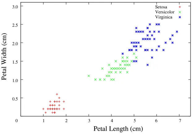
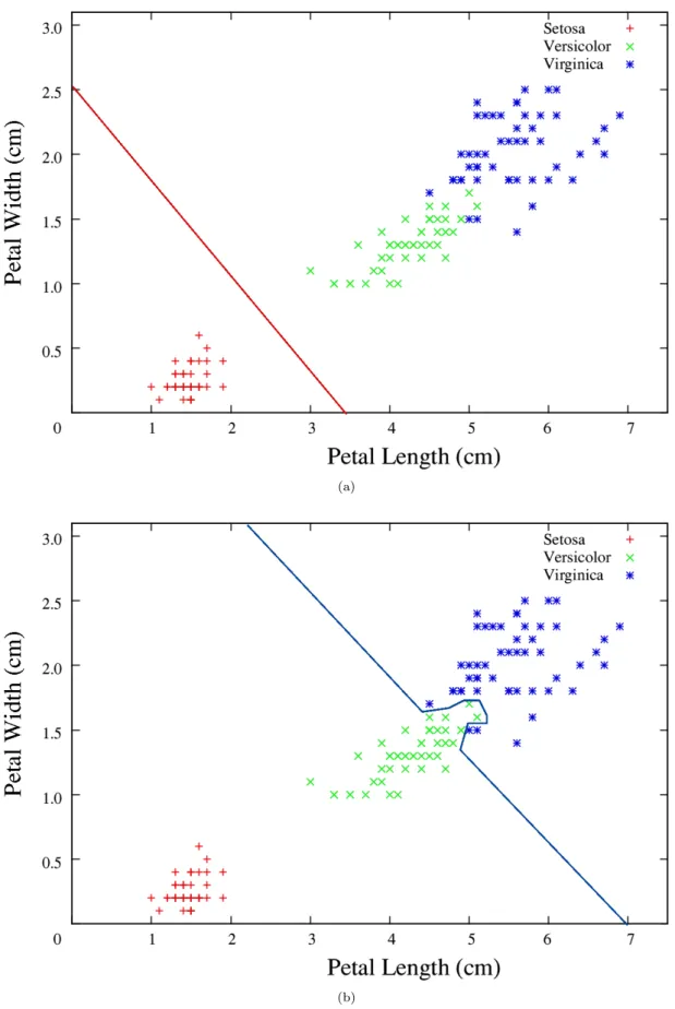
It is common to look at the classification problem geometrically. The goal of a classifier can be viewed as establishing a series ofclass boundaries, also known asdecision boundariesor decision surfaces, in the geometrical space populated by the data. This space may be referred to as theinput space, and has the same dimensionality as the data. New data points can then be classified depending on which side of the class boundaries they fall. For example, consider again the Iris dataset presented in figure 1.1. Whilst each record in this dataset corresponds to a different Iris plant, each of these plants is a member of one of three classes: setosa, versicolor or virginica [41], as shown in figure 1.3. One simple kind of class boundary that may be used

(a)

(b)

Figure 1.4: Class boundaries for the Iris dataset, separating (a) the setosa class from the versi-color and virginica classes, and (b) the virginica class from the setosa and versiversi-color classes.

in this two-dimensional dataset is a line, which is shown to separate the setosa and versicolor classes in figure 1.4(a). However, the separation between the versicolor and virginica classes is clearly nonlinear. A classifier could approximate this separation with a linear class boundary, but this would result in some misclassification of the data. A better approach would be to construct anonlinear class boundary, as shown in figure 1.4(b). The kinds of class boundaries that can be created depend on the particular classifier being used. Whilst the class boundaries may be referred to as lines or curves in two-dimensional space, in higher dimensions these same geometrical concepts are known as hyperplanes and hypersurfaces respectively. That is, when we talk about a hyperplane inn-dimensional space, we are simply referring to the same geometrical concept that is a line in two-dimensional space and a plane in three-dimensional space.

It is important to note that, whilst in the above example we drew the class boundaries whilst considering the entire dataset, in reality a classifier must decide the shape and position of these boundaries based on the training dataset alone. The more representative the training dataset is of the classes, the more likely it is that new data will be accurately labelled by the classifier. However, if the classifier fits the training data too closely, then it may give a poor performance on any new data it is faced with. This well-known problem is referred to asoverfitting and we consider this in more detail in chapter 5.

1.1.2

Cluster Analysis

Cluster analysis, or clustering, is a descriptive data mining task which finds groups, or clusters, of data within a dataset. Each data point belonging to a particular cluster is, in general, more similar, or related in some way, to the other data points in that cluster than to those in any other [113]. The clusters are constructed based on the information directly available from the data itself.

In many datasets, the notion of a cluster is not well defined since the data may be grouped in a variety of different ways, depending on what is most useful or meaningful in a particular scenario [113]. A cluster may simply be defined as a set of data points in which each data point is closer in some way to every other data point in the cluster than to any data point not in the cluster. Alternatively, cluster membership may be determined by a representative data point known as a prototype, whereby data points belong to the cluster if they are more similar to that cluster’s prototype than to any other prototype. Or, data density may instead be used, in which a cluster may be defined as a crowded (dense) region of data points surrounded by an

area of low density. Similarly, collections of clusters, known as clusterings, may be organised in different ways [113]. The clusters may be nested, in that a particular cluster may have one or more subclusters associated with it, or unnested. It may be useful to impose the restriction that a particular data point may only belong to a single cluster, or perhaps overlaps between clusters may be permitted. Finally, clusters might be formed over the entire dataset, or just a subset which excludes those observations that are uninteresting in some way.

Figure 1.5: Hyperspherical class boundaries in the Iris dataset.

Cluster analysis establishes groupings within datasets, which can subsequently be used to perform classification. The class label of a given data point is defined by the cluster to which that data point belongs [113]. For example, the majority of the data in the Iris dataset shown in figure 1.3 can clearly be grouped into three clusters, with each cluster representing a different class, as shown in figure 1.5. Since the clusters are inferred from the data directly, and no labelled examples are provided, a classifier based on cluster analysis is trained using an unsupervised learning process. The kind of class boundaries constructed naturally depends on the kind of clustering technique used. For example, a prototypical clustering approach may construct hyperspherical class boundaries around the data, such as those shown in figure 1.5 for the Iris dataset. As with the terms hyperplane and hypersurface, a hypersphere is simply the

generalisation of the geometrical concept of a sphere in three-dimensional space ton-dimensional space.

1.2

Novelty Detection

Consider again the example of the outdoor sensor network given at the start of this chapter. In this scenario one could establish a series of classes with each identifying a different weather condition, for example: sunny, cloudy, rain, gales, storm, etc. Examples of these classes could then be used to train a classifier to group new observations. But what about data that indicates some problem with the sensor nodes, such as becoming obstructed by animals or other objects in the environment, or a fault with a particular node itself? One could try to anticipate such occurrences and somehow derive characteristics that may be used to define additional classes on which the classifier may then be trained. But deriving the characteristics for a particular fault condition may be difficult without resorting to inducing that fault by deliberately damaging a sensor node in some way, which is clearly undesirable. Furthermore, how can one hope to anticipate each and every single possible fault that may occur? Clearly, rather than anticipating these occurrences, a better approach would be to identify deviations from known conditions. Is it possible to identify data that is unlike anything we would expect to see, using only our knowledge of the data that we are familiar with? This question motivates the study of novelty detection, which is the focus of this thesis.

Novelty detection is, in its most general form, the detection of data that is unusual or unknown, given some acquired knowledge. That is, novelty is defined in terms of what has been seen before [85]. For example, a single rotten apple in a basket of healthy apples could be considered as novel. Its class (rotten) goes against what we would expect (healthy), given that the vast majority of the apples in the basket are healthy (knowledge). However, if instead roughly half the apples in the basket are rotten then, based on that basket alone, we wouldn’t consider a rotten apple to be novel at all. This is because now our knowledge, defined by the basket, is that apples are just as likely to be rotten as they are healthy. But, if we considered this basket as one of a series of otherwise healthy baskets, then we might say that thebasket is novel. In this case, our knowledge, based solely on the previous healthy baskets, tells us that baskets should contain healthy apples. In the example of the outdoor sensor network given above, an observation would be considered novel if it represented an unusual weather condition or a fault of some kind. However, what constitutes an unusual weather condition may

depend on the timescale upon which the knowledge is based. If this knowledge is limited to 6 hours of measurements, for example, then events such as sunrise and sunset may be considered novel. Alternatively, with a knowledge consisting of 6 years of measurements, then typically only extreme weather conditions and uncommon faults would be highlighted as novel.

As mentioned in section 1.1, novelty detection is most related to the data mining tasks of classification and cluster analysis. A classifier is normally trained to recognise a finite set of known classes, and this training defines its knowledge, i.e. how to identify the class of a particular data point given the assumption that the data point belongs to one of the known classes. However, what if this assumption is false and the data point actually belongs to some unknown class? The classifier then has insufficient knowledge to correctly classify this anomalous data point. Worse still, since the classifier has no way of realising that its knowledge is insufficient, it may still attempt to classify the data point nonetheless, inevitably resulting in misclassification. However, as we will see in chapter 2, some approaches to classification have been proposed that can refuse to classify data points which seem unusual. By refusing to classify such data points, a classifier is then performing a kind of novelty detection in that it recognises that the data points are likely to belong to an unknown class. Cluster analysis is particularly interesting from the perspective of novelty detection, since it enables class boundaries to be constructed that surround data points, as opposed to partitioning the entire space. A data point not belonging to any of the known classes should fall outside the boundary of all clusters, and so can easily be identified as novel. A variety of different approaches to novelty detection based on cluster analysis techniques, such as Kohonen’s self-organising map (presented in chapter 2), have been proposed in the literature. However, many other approaches have also been proposed employing techniques from a wide range of different areas within machine learning. In chapter 2, we examine a wide selection of these different approaches.

From the perspective of classification, a data point may be considered novel if it does not belong to a known class. Such data points could also be referred to asanomalies, or outliers. Hence, many approaches to detecting them are commonly referred to as anomaly detectors or outlier detectors [47, 58]. Whilst the terms anomaly and novelty may be used interchangeably, the same is not necessarily true for outlier. It is possible that an outlier is still a member of a known class [104], meaning that the detection of outliers may not strictly be the detection of true novel or anomalous data points. Despite this, some authors still consider novelty/anomaly detection and outlier detection to refer to the same problem [47]. In this thesis, we are concerned with identifying novel, anomalous, entities alone. Novelty detection is also commonly referred to

asone-class classification, in recognition of the fact that a novelty detector is typically required to recognise both normal and novel data when trained on normal data alone. In this way, a novelty detector may be viewed as determining whether a particular data point lies inside or outside of the normal class. However, in some novelty detection tasks a limited amount of novel data is available to train the detector. For example, approaches to fraud detection sometimes use examples of data pertaining to fraudulent activity during the training phase [11]. These kinds of novelty detection tasks are beyond the scope of the work presented in this thesis.

1.2.1

Novelty Detection and Record Data

As mentioned in section 1.1, in the work presented in this thesis we consider novelty detection problems involving two kinds of data: record data and time series data. Many real-world applications store data in record datasets. For example, blood tests taken from a series of patients may be stored as a series of records, where each record corresponds to a different patient and each attribute represents a different measurement. In such a scenario, one could use a novelty detector to identify patients whose blood test data indicates the possible presence of disease. Similarly, measurements taken from breast masses from a number of patients may be stored as a record dataset, and a novelty detector could then be used to identify those masses which may signify the presence of breast cancer.

In a record dataset, no ordering or temporal information exists between the data elements [113]. This means that a novelty detector must decide whether or not a particular data element is novel using only the knowledge it has acquired during a training phase. Each data element normally requires a separate decision, which may be associated with it in the same way as a class label in a classification problem. A novelty detector may be thought of as predicting the class label of each dataset, where the available classes to choose from are “normal” and “novel”.

1.2.2

Novelty Detection and Time Series Data

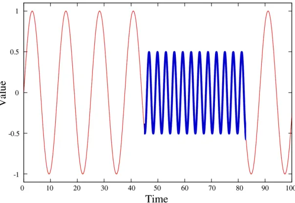
Novelty detection is also commonly used to detect unusual, or novel, events in time series data. For example, novelty detection is frequently used as an approach to fault detection [32], that is identifying faults or breakdowns in mechanical systems. It has also been used in tasks such as identifying unusual heartbeats from patients with arrhythmia [7, 68], detecting anomalies in computer network traffic [3] and detecting unusual features of an indoor environment explored by a mobile robot [85]. In many cases, a novel event consists of some number of data points

Figure 1.6: An example time series with the presence of a single novel event (highlighted in blue).

which deviate from the normal behaviour of the series. Again, these are also referred to by some authors as anomalies, or outliers [112]. An example of a novel event in a time series is shown in figure 1.6. The highlighted novel points do not fit the normal behaviour of the remaining points in the series. A novelty detector may respond by labelling every one of these points as novel, in the same way it does for record data, or it may highlight theevent instead, i.e. providing a real-time alarm as early as possible during the onset of the event. The most appropriate way of flagging novel data points depends on the particular scenario being considered.

Change Detection

When dealing with data that has a temporal component, one may naturally be interested in identifying some form ofinteresting change in that data. In some cases, any change might be interesting as it may be unusual or unexpected. On the other hand, data may be undergoing constant change over time. In this case, what constitutes an interesting change would depend on the application.

of time series data [30]. Abrupt change-point detection, or simply change-point detection, is concerned with identifying those points at which a sudden change occurs in the properties of the data [30]. A change may be persistent, thus yielding a single change-point, or multiple change-points may exist in the series. Change-point detection is also referred to as time series segmentation [128], since the change-points delimit segments of the series in which data has common properties. Since a novel event in a time series, such as that shown in figure 1.6, does exist as a segment, with different properties to the remainder of the series, they can be identified by change-point detection methods. However, depending on the application, a time series segment may not necessarily represent a novel event. For example, a musical composition consists of numerous segments, each corresponding to a different musical note [30]. Whilst a note might represent a novel event (e.g. if it has not been used before, or it differs from the note specified on the written score), the majority of notes naturally do not. In applications where abrupt change is always indicative of novelty, change-point detection may be used as an approach to identify novel events.

Other forms of change detection have also been proposed. For example, Forrestet al. consider the problem of detecting changes, possibly caused by viruses, in computer files [43]. In this scenario, the content of the files should remain static and so any change is considered unusual, or novel. Alternatively, Fanget al. examine the problem of identifying changes in video sequences taken from the windscreen of a car travelling along a highway [38]. Here, as the authors point out, change is constantly occurring in the video sequence. The kinds of change that are interesting in this scenario are those which could have an impact on driver safety.

Forgetting

Another challenge one is faced with when identifying anomalies in time series data is that the environment from which the time series is generated may change over time. Events which were previously uncommon may become commonplace, and therefore change their status from being novel to being normal. For example, in the time series produced by a sensor measuring outdoor temperature, a period of time in which the temperature is above 25◦C may be considered a normal event during the summer months, but novel during the winter. The time series measured by the temperature sensor exhibits seasonal variations, where the normal conditions change over time. In such applications, an important quality of a novelty detector is the ability to “forget” about events witnessed in the distant past, basing its concept of normality on what has been seen “recently”. The period of time that defines “recent” again depends on the application.

1.3

Challenges of Applying Novelty Detection to a

Partic-ular Scenario

Novelty detection is used in wide range of different real-world problems, such as identifying possible signs of cancer, detecting irregular heart beats, identifying evidence of intrusions in a computer network and detecting faults in mechanical machinery. It is a useful technique in any problem which involves identifying small amounts of unusual, novel, data from large amounts of uninteresting, normal, data. As we will show in chapter 2, many existing approaches to novelty detection tend to focus on one specific problem or group of problems. By doing so, these approaches can be tailored to exploit the unique properties of the chosen problem(s) to achieve a good performance. These approaches also tend to require the definition of a number of parameters, whose values critically impact on performance.

In many real-world scenarios in which novelty detection is required, it is likely that the user, the person wishing to utilise the novelty detector, is not an expert in either novelty detection or the data mining field in general. However, they are likely to have an expert knowledge of their particular problem. For such a user, employing a novelty detector presents significant challenges. First, they must decide on an existing approach which is suitable for their problem. Unless their problem is similar enough to one which has been used to demonstrate the performance of a particular novelty detector in the literature, the user will themselves need to evaluate those approaches they consider to be promising. Once a novelty detector has been selected, the user must decide appropriate values for any parameters that it may have, which is typically a trial-and-error process. These challenges are at best time consuming and at worst prohibitively difficult for the user. It is also possible that their problem is so unusual that no suitable approach exists, in which case the user’s only option would be to construct a new specialist novelty detector, a task which requires expert knowledge.

In order to make novelty detection more accessible, an approach is required which does not pose the above challenges. It should be capable of performing novelty detection in a wide range of different scenarios, without requiring expert knowledge from the user. It should also not require a large amount of time from the user in setting it up for a particular novelty detection task, and it should operate efficiently and effectively in that task. But, with the seemingly infinite number of real-world scenarios, involving data with vastly different properties, is this really achievable? To attempt to answer this question, we focus on developing such an approach in this thesis.

1.4

Aims and Objectives

The aims of the work presented in this thesis can be succinctly described by the following sentence:

To develop an approach which enables novelty detection to be performed easily, effi-ciently and effectively in a wide range of different scenarios.

From these aims, we may derive a number of objectives that the approach must achieve. Firstly, it should begenerally suitable for use in a wide range of different novelty detection problems. To accomplish this, the approach should minimise the assumptions it makes about the nature of the problems to which it will be applied. For example, a novelty detector designed specifically for use with time series data would naturally be unsuitable for use in problems involving record data. Alternatively, a detector might assume that the underlying distribution of the data is Gaussian. Whilst this may not prevent the detector from being physically applied to a problem in which this assumption is untrue, it would be unlikely to achieve an effective performance. Assuming that the approach is not physically unsuitable for use in a particular novelty detection task, its performance is a natural indicator of its suitability for solving that task.

The general suitability of the approach will also depend on how much it may becustomised to the novelty detection task at hand. However, whilst this customisability is important, it often has an impact on the amount of work, or effort, required by the user for configuration. For example, many novelty detection approaches in the literature may be customised by a series of parameters, whose values critically determine their performance. This significantly increases the effort required by the user, since a time consuming search of the parameter space must be performed. As stated above, the approach we aim to develop should be easy for the user to apply to a particular novelty detection task, and so it should minimise the amount of work required.

Finally, the complexity of the approach should be no more than is required for the particular novelty detection task to which it is to be applied. It should not have properties that are redundant or unnecessary in the context of that task. To some extent, this might be achieved by exploiting the unique properties presented by the data on which the task is based. This constraint prevents us from considering monolithic systems which comprise a multitude of different novelty detection techniques. These systems are undesirable since they would require more resources than an effectively tailored novelty detector, which could prohibit their use in some cases.

To summarise, the approach we aim to develop in this thesis must achieve the following objectives:

• General Suitability: The approach should be suitable for and effective in a wide range of different novelty detection tasks.

• Customisability: The approach should permit a high degree of customisability.

• Work: The effort required from the user to customise the approach for a particular task should be minimal.

• Complexity: The complexity of the approach should be justifiable for the particular task. We use these objectives to systematically evaluate both existing approaches to novelty detection in the literature (chapter 2) and the approach we propose in this thesis (chapters 5 and 6).

1.5

Contribution of this Work

The main contribution of this thesis is the development of a new approach to novelty detection which attempts to satisfy the objectives outlined above. This approach combinesDynamic Pre-dictive Coding (DPC), a biologically inspired neural network model proposed by Hosoya et al. [63], with Stanley’sNeuroevolution of Augmenting Topologies (NEAT) method [108], an evolu-tionary algorithm specifically designed to evolve neural networks of any topology. The proposed approach, DPC+NEAT, aims to satisfy the above objectives by automatically constructing neu-ral network novelty detectors for particular scenarios. By freely designing a suitable network structure, as well as selecting values for the network’s parameters, the approach has the poten-tial to produce highly customised detectors that perform effectively, whilst requiring a minimal amount of work from the user. By introducing new network structure slowly through the course of evolution, the approach also has the potential to construct novelty detectors which have a justifiable level of complexity for the task at hand.

In order to gain insight into its potential effectiveness, we first examine the performance of the proposed approach in a test scenario, based on the problem for which the DPC model was originally devised. We examine the effect of allowing DPC+NEAT to choose the values of the parameters of the neural network in addition to its structure, as well as observing the impact of artificial noise on the performance of the approach. We then evaluate DPC+NEAT in a number of different novelty detection tasks, over both record and time series datasets. The performances

of the detectors evolved for each task are compared against that given by a number of existing approaches to novelty detection in the literature. From this evaluation, we assess the success of DPC+NEAT in meeting the aims of this research.

1.6

Summary

We have introduced the data mining task of novelty detection, initially from the perspective of classification, and described a number of different forms of novelty that may occur. In data with no temporal component, novel data points are those which do not fall into any of those classes knowna priori. However, in data with a temporal dimension, one may be interested in different forms of novelty, such as those points in a time series which indicate some significant change has occurred, or unexpected changes in usually static data.

Novelty detection may be extremely useful in many different real-world problems which involve identifying small amounts of unusual, novel, data from large amounts of uninteresting, normal, data. However, for the non-expert user it may be prohibitively difficult to utilise an approach to novelty detection in their particular scenario. Not only must they identify and evaluate a suitable approach, they also need to configure this approach to enable a good performance. A system that allows novelty detection to be easily, efficiently and effectively applied to a particular problem would not pose such challenges to the user, and thus would make novelty detection more accessible.

In this thesis, we present an approach which aims to allow novelty detection to be eas-ily, efficiently and effectively performed in a wide range of different scenarios. This approach, DPC+NEAT, automatically constructs a neural network novelty detector which is highly cus-tomised for the particular novelty detection task at hand. We have discussed four objectives that the proposed approach should accomplish in order to satisfy the aim of this research, and we use these objectives as an evaluation criteria for our proposed approach in chapters 5 and 6.

1.7

Overview of the Thesis

We now provide a brief overview of the remainder of this thesis:

Chapter 2surveys the current existing approaches to novelty detection in the literature and evaluates each approach against the objectives derived in section 1.4. We establish that none of the approaches fulfils all of these objectives, thus justifying the need for a new approach.

Chapter 3 describes Hosoyaet al.’s DPC neural network model [63], which was originally proposed to explain a phenomenon observed in the neural pathways of the retina. However, the model can also be viewed as performing a kind of novelty detection over visual images. One drawback of the model is that it does not define a specific network topology, which must instead be tailored manually to the particular application. Therefore, we also examine algorithms capable of automatically evolving the topology and weights of a neural network. Of these algorithms, we find that Stanley’s [108], Neuroevolution of Augmenting Topologies (NEAT) approach overcomes or avoids a number of key problems faced when evolving neural networks. The DPC model and the NEAT method form the basis of our proposed approach to novelty detection presented in this thesis.

Chapter 4presents our proposed DPC+NEAT approach. We combine Hosoyaet al.’s DPC model with Stanley’s NEAT algorithm to construct a system which is capable of automatically evolving neural network novelty detectors for specific applications. We examine the performance of the system in a test scenario, and propose a series of modifications to allow the system to construct novelty detectors for other kinds of novelty detection tasks.

Chapter 5 evaluates DPC+NEAT according to the objectives given in section 1.4. The system is used to find detectors in a number of very different novelty detection tasks, over both record and time series datasets. We also compare the performance of the detectors with a number of the approaches surveyed in chapter 2.

Chapter 6concludes this thesis. A summary of the work is presented, and the drawbacks of the proposed DPC+NEAT approach are discussed. These drawbacks define a number of directions in which this work may be extended. In light of the drawbacks identified, we consider whether or not DPC+NEAT successfully meets the aims of this research. We also present other ideas on how the proposed approach may be further improved.

Existing Approaches to Novelty

Detection

In this chapter, we evaluate a range of existing approaches to novelty detection from the literature against the objectives stated in chapter 1. We demonstrate that no existing approach successfully fulfils all four objectives, thus justifying the need for a new approach. We also identify a technique applied to novelty detection that has the most potential for fulfilling these objectives.

2.1

Introduction

As we have described in chapter 1, novelty detection refers to the problem of identifying those data elements that are unusual in some way given some acquired knowledge on the state of normality. This could be viewed as the two-class classification problem of determining whether each data element presented belongs to thenormal ornovel class. However, unlike a two-class classifier, which is provided with information about both classes, a novelty detector is usually only given information on the normal class alone. This is due to the fact that, whilst a large quantity of normal data can be easily provided in a given scenario, there tends to be very few examples of the novel class available.

A large variety of different approaches to the problem of novelty detection have been pro-posed in the literature. These generally fall into one of two groups: statistical approaches and neural network approaches [83, 84]. Statistical approaches to novelty detection may be further subdivided intoparametric andnon-parametric methods. Parametric statistical methods make

strong assumptions about the underlying distribution of a population: typically this assumption is that the distribution is Gaussian. Non-parametric approaches make no assumptions about the distribution and are therefore more flexible [83]. Neural network approaches cover a wide variety of different types of neural network. These include multilayer perceptron networks, au-toassociators, radial basis function networks, self-organising maps, adaptive resonance theory networks and evolutionary neural networks.

The approaches that we examine in this chapter use different kinds of learning strategies. Some approaches employ anoffline learning strategy, in which a model of the normal class is derived during a training phase involving a specially provided training dataset. The learning technique may be supervised or unsupervised in this case, depending on whether or not labels can be assigned to the training data. The quality of the knowledge acquired by the learner may then be assessed through a test phase, in which the learner is evaluated over a test dataset consisting of data not seen during training. Alternatively, some approaches performonline learning, where the training phase takes place in-situ using real data taken directly from the novelty detection task at hand. This generally requires an unsupervised learning technique to be used, since the data is not usually labelled. For the same reason, a test phase is generally not feasible either. Naturally, an online learning approach can also be applied to a scenario in which offline learning is required. An approach capable of online learning may also supportadaptive learning, where it continuously learns about the data and is able to adapt to any changes in the properties of this data. This learning strategy may permit an approach toforget about properties of the data that have not been recently observed. Such an ability is especially important in those time series scenarios in which normality is defined in terms of the recent past. An adaptive learning strategy is generally the most flexible since this adaptive capability can normally be easily disabled when not required in a particular scenario and, since it performs online learning, can also be applied to scenarios in which an offline learning strategy is required.

In chapter 1, we described four objectives that an approach which could be used to easily, efficiently and effectively perform novelty detection in a wide range of scenarios should fulfil. The approach should be (1)generally suitable for use in a wide range of different novelty detection tasks, (2) permit a high degree ofcustomisability, (3) minimise thework required from the user in configuring it for use in their particular scenario and (4) have a level ofcomplexity that is justifiable for the novelty detection task to which it is being applied. In this chapter, we evaluate a range of approaches to novelty detection from the literature against these objectives. We find that no existing approach is capable of fulfilling all four objectives, therefore demonstrating the

need for a new approach. In the next section, we review non-parametric statistical approaches to novelty detection. In section 2.3, we change our focus to neural network approaches. We conclude this chapter in section 2.4 with a summary of this review.

2.2

Statistical Approaches to Novelty Detection

Statistical approaches to novelty detection tend to model training data based on its statistical properties, and then use this model to determine whether or not elements from the test set appear to belong to the same distribution [83]. They may be subdivided intoparametric approaches, which assume that the data comes from a family of known distributions, andnon-parametric approaches, in which the distribution of the data, as well as any associated parameters of this distribution, is inferred from the data itself [83]. Since parametric approaches are only suitable in applications where the assumptions made on the distribution of the data hold, their suitability for different novelty detection applications is clearly limited and so they are not considered here. Instead, we review the non-parametric approaches, which have a much wider applicability.

2.2.1

k

-Nearest Neighbour

The first non-parametric approach that we consider isk-nearest neighbour (KNN). This tech-nique classifies data points based on theirknearest neighbours in the input space, with respect to some distance measure (such as Euclidean distance). During the training phase, the KNN technique simplystores labelled training data points. All of the computational work required for the classification of testing data points takes place when those data points are presented for classification [90]. When classifying individual data points, a common rule is to assign those data points to the class in which the majority of theirk nearest neighbours belongs [90], with each neighbour having an equal influence on the classification. Alternatively, the influence of the neighbours may be weighted according to distance, such that those neighbours which lie closer to the data point being classified are assigned a higher weight than other points lying further away [90].

One way of applying the KNN technique to novelty detection is to assume that a novel data point will lie at a considerable distance from the training data points. This approach is used by Guttormssonet al. [52], who compared KNN with three other novelty detection methods for the task of identifying faults in a turbine generator. With the KNN technique, a data point is declared novel if the distance to its closest neighbour exceeds some decision threshold.

Therefore, a hyperspherical decision boundary is established around each training data point, whose radius is the decision threshold. However, in the novelty detection task considered in the study, the authors found that an alternative approach, which constructed a hyperelliptical boundary around the data, gave the best performance. This is because the data in the considered task is spread in an elliptical cloud, causing approaches based on spherical boundaries to classify too large a region of the input space as normal.

Another method of employing KNN for novelty detection was proposed by Tax and Duin [116]. For a particular test data pointx, an estimate of its likelihood p(x) may be calculated based on the volume of the sphere, centred onx, containing theknearest neighbours ofx[33]. Fork = 1, this is shown to be equivalent to the quotient of two Euclidean distance measures [116]: the distance between x and its nearest neighbour, N N(x), and the distance between this neighbourN N(x) and its own nearest neighbourN N(N N(x)). If this estimate is below a predefined threshold, then x is considered to be novel. In a task identifying vibration signals indicating damage in a submersible water pump, the proposed KNN method was shown to outperform three other novelty detection approaches. However, when the dimensionality of the dataset was reduced, the performance of the KNN method deteriorated.

Yang et al. [129] applied a nearest neighbour approach to the problem of First Story De-tection (FSD), a form of novelty deDe-tection used in the field of text mining. FSD refers to the problem of identifying the earliest reports of new events from chronologically ordered documents (such as newswire stories or television broadcasts [129]). Each event may be classified into one of a number of known topics, for example the event“1996 TWA Flight 800 crash” may be placed into the topic“aeroplane accidents”. Since what constitutes a new event changes over time, any approach to FSD must operate in an adaptive manner, updating its model of the normal class each time a new event occurs. The approach proposed by Yanget al. first classifies an incoming event into one of a series of topics. For each topic, an FSD algorithm based on KNN is then used to determine the novelty of the event. In a history of all past events, the nearest neighbour to the incoming event, according to some similarity score, is identified. The similarity between the incoming event and its nearest neighbour is then thresholded, with the incoming event being labelled as novel if these two events are not sufficiently similar. When applied to a benchmark dataset, the method was shown to give a very good performance.

Another approach to novelty detection based on KNN was proposed by Angiulli [5]. For a given input vector, this approach, called Nearest Neighbour Domain Description (NNDD), generates a vector holding the distances between the input vector and itsknearest neighbours.

If this vector falls outside of the hypersphere centred at the origin of_Rk _{with radiusθ, then the}

input vector is labelled as novel. Angiulli also proposed an extension to NNDD, which tackles an important drawback of the KNN technique: in order to classify a given input vector, KNN must compare that vector with each element of the training set which, in applications with large training sets, becomes computationally expensive. The proposed extension to NNDD, Condensed NNDD (CNNDD), selects a subset of the elements of the training set such that when trained with these elements NNDD is able to correctly classify all elements of the training set as normal. This subset is constructed with only two passes of the training set. The CNNDD approach was shown to outperform three other novelty detection methods, including Tax and Duin’s approach discussed above [116], over a number of benchmark datasets.

Evaluation

The KNN technique has been successfully applied to a variety of different novelty detection tasks. It has also been used in an adaptive fashion, being able to continuously update its con-cept of normality [129]. However, this adaptive variant of KNN was not capable of forgetting, and classification would therefore become increasingly computationally intensive as more data elements are presented. A significant drawback of the KNN technique is that it uses an over-complicated representation of the normal class, consisting of the entire training set. This level of complexity is unjustifiable in the majority of novelty detection tasks, in which a decision boundary would be sufficient to separate the normal and novel classes. However, this drawback has been tackled by condensing the training set to its key elements [5], with promising results. But employing this condensing approach whilst allowing the novelty detector to continuously learn about its environment has not yet been demonstrated.

Another drawback of the nearest neighbour approach is that it is especially sensitive to the curse of dimensionality [90]. The distance measure used is based on all attributes of the data, whilst in reality a large number of these attributes may provide no information on whether or not a data instance is normal or novel. In this case, the large number of irrelevant attributes may distort the calculated distance between data instances. To avoid this problem, some form of feature selection or dimensionality reduction technique, such as principal component analysis, may first be applied to the data. For applications involving high-dimensional data, this increases the complexity of the approach. Alternatively, an attribute weighting strategy could be used to highlight those attributes which are more relevant than others. However, finding the optimum weight for an attribute is again a complex problem [101].

2.2.2

Negative Selection

Novelty detection has also been considered in the domain of artificial immune systems (AIS). The biological immune system is capable of identifying virtually any foreign cell or molecule [43]. To accomplish this, it produces T cells which have receptors that can detect foreign proteins, referred to as non-self. The receptors are created through a pseudo-random genetic process, and so it is likely that some receptors are produced which bind to the body’s own cells, known asself. Therefore, T cells undergo a selection process, callednegative selection, where those T cells with receptors which bind to self are destroyed leaving only those T cells which identify non-self, which are then released.

Forrestet al. [43] first proposed an approach based on negative selection to perform change detection over computer files, in order to detect computer viruses. In this approach, the data to be protected is represented as a string in some alphabet, which is referred to as the self string. This self string is then divided into equal size segments to produce the collection of self strings S. A series of random strings are then generated and tested against each element of S. If a random string matches any element in S (i.e. matches self), it is rejected. Otherwise, it is deemed to match non-self and so is placed in a non-self detector collection R. Two strings are considered to match if they havercontiguous matches at the same locations. Once the collection of detectors has been constructed, the collection S is then monitored by continuously matching strings in S with detectors in R. If a match occurs, then the corresponding element in S has changed in some way. Using a binary string representation, the approach was shown to perform well at detecting changes made to compiled program files.

Gonz´alez et al. [47, 48] generalised the negative selection algorithm to real space. In this approach, which they called real-valued negative selection (RVNS), a series of self samples, represented asn-dimensional vectors, are used as input. The area of the input space in which these samples lie is referred to as theself space, whilst the remaining areas of the input space constitute the non-self space. RVNS then proceeds by first generating a random collection of detectors, also n-dimensional vectors, and then evolving these detectors so that they do not match any of the self samples. A match occurs if a self sample falls within a specified radiusr of a detector, indicating that the detector overlaps the self space. If a detector matches a self sample, then it is moved in a direction away from the self space. Each time a match occurs for a particular detector, the age of that detector is increased. Detectors whose age is greater than some threshold are subsequently replaced with new random detectors. The authors combined