Gaussian Processes for Temporal and Spatial Pattern
Analysis in the MISR Satellite Land-Surface Data
A dissertation submitted to the Faculty of Science,
University of the Witwatersrand, Johannesburg,
in fulfilment of the requirements for
the degree of Master of Science
Adrian John Cuthbertson
Supervisor: Professor Clint van Alten
School of Computer Science
Abstract
The Multi-Angle Imaging SpectroRadiometer (MISR) is an Earth observation instrument operated by NASA on its Terra satellite. The instrument is unique in imaging the Earth’s surface from nine cameras at different angles. An extended system MISR-HR, has been developed by the Joint Research Centre of the European Commission (JRC) and NASA, which derives many values describing the interaction between solar energy, the atmosphere and different surface characteristics. It also generates estimates of data at the native resolution of the instrument for 24 of the 36 camera bands for which on-board averaging has taken place prior to downloading of the data. MISR-HR data potentially yields high value information in agriculture, forestry, environmental studies, land management and other fields. The MISR-HR system and the data for the African continent have also been provided by NASA and the JRC to the South African National Space Agency (SANSA). Generally, satellite remote-sensing of the Earth’s surface is characterised by irregularity in the time-series of data due to atmospheric, environ-mental and other effects. Time-series methods, in particular for vegetation phenology applications, exist for estimating missing data values, filling gaps and discerning periodic structure in the data. Recent evaluations of the methods established a sound set of requirements that such methods should satisfy. Existing methods mostly meet the requirements, but choice of method would largely depend on the analysis goals and on the nature of the underlying processes. An alternative method for time-series ex-ists in Gaussian Processes, a long established statistical method, but not previously a common method for satellite remote-sensing time-series. This dissertation asserts that Gaussian Process regression could also meet the aforementioned set of time-series requirements, and further provide benefits of a consis-tent framework rooted in Bayesian statistical methods. To assess this assertion, a data case study has been conducted for data provided by SANSA for the Kruger National Park in South Africa. The re-quirements have been posed as research questions and answered in the affirmative by analysing twelve years of historical data for seven sites differing in vegetation types, in and bordering the Park. A further contribution is made in that the data study was conducted using Gaussian Process software which was developed specifically for this project in the modern open language Julia. This software will be released in due course as open source.
Declaration
I declare that this dissertation is my own unaided work, except where otherwise
acknowledged. It is being submitted to the University of the Witwatersrand, Johannesburg, for the degree of Master of Science. It has not been submitted before for any degree or examination in any other university.
Adrian John Cuthbertson 30th May 2014
Acknowledgements
I would like to acknowledge and thank my supervisor Professor Clint van Alten who accom-panied me on this journey into these fascinating domains and provided a sound guiding hand along the way.
I would like to thank the staff of SANSA who provided the MISR-HR data and offered their time in answering questions on technical details of the MISR-HR system. In particular Dr Michel Verstraete, Linda Kleyn and Dr Nicky Knox. Also to Linda Hunt of Science Sys-tems and Applications, Inc., Hampton, VA, United States, for also answering queries about the MISR-HR system. Also to Dr Bob Scholes of the CSIR, who introduced me to the MISR-HR system and outlined its vast potential.
I would like to also thank Dr Michel Verstraete for the opportunity of contributing a slide on my work on the MISR-HR data for his keynote address to the American Geophysical Union Conference in December 2013.
Contents
1 Introduction 6
2 Research Background 9
2.1 The MISR Satellite Instrument . . . 9
2.2 The MISR-HR System . . . 11
2.2.1 Models and Products . . . 12
2.2.2 Datasets . . . 13
2.3 Time-Series Methods in Satellite Remote-Sensing . . . 14
2.3.1 The Smoothing Spline Method . . . 14
2.3.2 The Singular Spectrum Analysis (SSA) Method . . . 15
2.3.3 The Lomb-Scargle Method . . . 15
2.3.4 Criteria for Choices of Time-Series Methods . . . 16
2.3.5 Comparing Goodness-of-Fit . . . 16
2.3.6 Other Methods Recently Studied . . . 17
2.3.7 Conclusions . . . 17
2.4 Gaussian Processes . . . 18
2.4.1 Supervised Machine-Learning Parametric Methods . . . 18
2.4.2 Gaussian Process - A Bayesian Non-Parametric Method . . . 19
2.4.3 Goodness-of-Fit - The Negative Log Likelihood . . . 20
2.4.4 GP Regression Example . . . 21
2.4.5 Covariance Kernels . . . 24
2.4.6 GP Hyper-Parameter Learning . . . 28
2.4.7 Gaussian Process Algorithms Toolkit . . . 29
2.5 Software Components and Libraries . . . 29
2.5.1 The Julia Scientific and Technical Programming Platform . . . 29
2.5.2 MISR-HR Data Processing - EOS.jl Component . . . 30
2.5.3 Gaussian Process Implementation - The GP.jl Component . . . 31
2.5.4 Results Plotting - Julia and Python Matplotlib Libraries . . . 31
2.5.5 Time-Scale Model . . . 31
2.6 Conclusions . . . 34
3 Research Problem, Thesis and Methodology 35 3.1 The Research Problem . . . 35
3.2 The Thesis . . . 35
3.3 Research Methodology . . . 36
3.4 Research Questions . . . 36
4 Gaussian Process Time-Series on MISR-HR Data 38 4.1 Smoothing Time-Series . . . 38
4.1.1 Raw Time-Series . . . 38
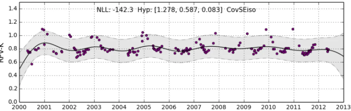
4.1.2 CovSEiso Kernel - Default Hyper-Parameters . . . 39
4.1.3 CovSEiso Kernel - Optimised Hyper-Parameters . . . 40
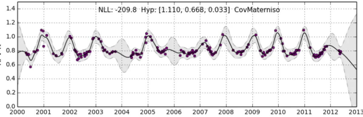
4.1.4 CovMaterniso Kernel - Optimised Hyper-Parameters . . . 40
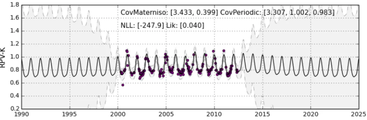
4.2 Periodic Structure and Forecasting . . . 41
4.2.1 Composite Kernel - CovMaterniso and CovPeriodic Summed . . . 41
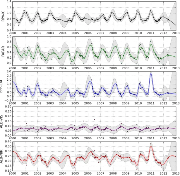
4.2.2 Comparing Smoothing and Composite Periodic over other MISR-HR fields . . . 44
4.3 Conclusions . . . 47
5 MISR-HR Data Case Study 48 5.1 Kruger National Park Sites Chosen For GP Models . . . 48
5.2 Modelling Methodology . . . 49
5.3 Geolocation, Block and Dataset Selection . . . 49
5.4 Target Site Identification . . . 51
5.4.1 Data Extraction and Processing . . . 52
5.5 Composite Periodic Models For all Sites . . . 52
5.6 Comparing Sites E1, E2, E3, E4 in Different Landscapes . . . 60
5.7 Comparing Sites E3, F1, F2, H1 for Fire and Human Development . . . 61
5.8 General Observations From Site Model Plots . . . 63
5.9 Conclusions . . . 67
6 Conclusions 70 6.1 Summary . . . 70
List of Figures
2.1 MISR Satellite Instrument Schematic. . . 11
2.2 Sample regression model - Squared Exponential covariance function. . . 22
2.3 GP Prior Samples Drawn from a Squared Exponential Kernel - Example 1 . . . 25
2.4 GP Prior Samples Drawn from a Squared Exponential Kernel - Example 2 . . . 26
2.5 GP Prior Samples Drawn from a Mat´ern Kernel - Example 1 . . . 26
2.6 GP Prior Samples Drawn from a Mat´ern Kernel - Example 2 . . . 27
2.7 GP Prior Samples Drawn from a Periodic Kernel - Example 1 . . . 27
2.8 GP Prior Samples Drawn from a Periodic Kernel - Example 2 . . . 28
4.1 Raw Time Series for RPV-K with Outliers . . . 39
4.2 Smoothed Time-Series - CovSEiso with Defaults . . . 39
4.3 Smoothed Time-Series - CovSEiso Optimised . . . 40
4.4 Smoothed Time-Series - CovMaterniso Optimised . . . 41
4.5 Composite Kernel Periodic Time-Series - Initial Optimise . . . 42
4.6 Composite Kernel Periodic Time-Series - Optimised . . . 43
4.7 Composite Kernel Periodic Time-Series - Long-Term . . . 43
4.8 Site E1 Full Plate - CovMaterniso . . . 45
4.9 Site E1 Full Plate - Composite Periodic . . . 46
5.1 Overlapping Orbit Blocks . . . 49
5.2 Composited MISR-HR Image for Block 169/109, 2010-08-18 . . . 50
5.3 Composited MISR-HR Image for Block 170/109, 2010-08-09 . . . 50
5.4 Image Showing Study Area and Target Sites . . . 51
5.5 Site E1 Full Plate - Mopane Savannah . . . 53
5.6 Site E2 Full Plate - Sandveld Communities . . . 54
5.7 Site E3 Full Plate - Mopani/Bushwillow Woodlands . . . 55
5.8 Site E4 Full Plate - Mopani Shrub Veld . . . 56
5.9 Site F1 Full Plate - Fire Site 1 . . . 57
5.10 Site F2 Full Plate - Fire Site 2 . . . 58
5.11 Site H1 Full Plate - Human Development . . . 59
5.12 Sites E1, E2, E3, E4 - RPV-K . . . 60
5.13 Sites E1, E2, E3, E4 - FAPAR . . . 60
5.14 Sites E1, E2, E3, E4 - EFFLAI . . . 61
5.15 Sites E1, E2, E3, E4 - ALBEDO-NIR . . . 61
5.16 Sites E3, F1, F2, H1 - RPV-K . . . 62
5.17 Sites E3, F1, F2, H1 - FAPAR . . . 62
5.18 Sites E3, F1, F2, H1 - EFFLAI . . . 63
5.19 Sites E3, F1, F2, H1 - ALBEDO-NIR . . . 63
5.21 Site E1 - Minimum/Maximum - RPV-K . . . 65
5.22 Site E1 - Sequential Minimum/Maximum - FAPAR . . . 66
5.23 Fire Patches 2009-09-16 and 2010-07-17 . . . 68
5.24 Fire Patches 2010-09-19 and 2010-10-21 . . . 68
List of Tables
2.1 Covariance Kernels . . . 31
4.1 RPV-K Predictions - Solstice and Equinox Dates, Composite Periodic . . . 44
4.2 MISR-HR Fields and Descriptions . . . 44
4.3 Site E1 Full Plate Hyper-parameters - CovMaterniso . . . 46
4.4 Site E1 Full Plate Hyper-parameters - Composite Periodic . . . 47
5.1 Study Target Sites . . . 52
5.2 Site E1 Full Plate Hyper-parameters - Mopane Savannah . . . 53
5.3 Site E2 Full Plate Hyper-parameters - Sandveld Communities . . . 54
5.4 Site E3 Full Plate Hyper-parameters - Mopani/Bushwillow Woodlands . . . 55
5.5 Site E4 Full Plate Hyper-parameters - Mopani Shrub Veld . . . 56
5.6 Site F1 Full Plate Hyper-parameters - Fire Site 1 . . . 57
5.7 Site F2 Full Plate Hyper-parameters - Fire Site 2 . . . 58
5.8 Site H1 Full Plate Hyper-parameters - Human Development . . . 59
5.9 Site E1 Alternating Minimum/Maximum RPK-K Dates/Values . . . 66
Chapter 1
Introduction
The Multi-Angle Imaging SpectroRadiometer (MISR) is an Earth observation instrument operated by NASA on its Terra satellite [Diner et al.2002]. This instrument is unique in that it comprises nine cameras, imaging the same locations on the Earth’s surface from different angles distributed along the track of the satellite, providing multi-angled reflectance factors in electromagnetic bandwidths suitable for many applications.
A system known as MISR High Resolution or MISR-HR [Verstraeteet al.2012] has been developed by scientists at the Joint Research Centre of the European Commission (JRC) in Italy and implemented as a software package by Linda Hunt at the NASA Langley Atmospheric Science Data Centre in Virginia, USA. The purpose of the MISR-HR system is to derive many additional data values describing the interaction between solar energy, the atmosphere and the Earth’s surface. It also generates estimates of data at the native resolution of the instrument (275 m) for 24 of the 36 camera bands for which on-board averaging (to 1.1 km) has taken place prior to downloading of the data. The MISR-HR data is useful in fields such as agriculture, forestry, environmental studies, land management and others.
The scale of the MISR-HR data and their value is highlighted by the following analogy: the MISR-HR system could also be viewed as a virtual collection of many thousands or even millions of independent instruments positioned above every 275 metre square area of the planet’s surface, taking snapshot mea-surements and computing over 100 useful metrics for that square, from 3 to 10 times a month depending on the latitude.
During 2010, scientists from NASA, the JRC and the Council for Scientific and Industrial Research (CSIR) in South Africa, carried out field validations of MISR-HR in the Kruger National Park. With the success of this project, the MISR-HR system was made available by the JRC and NASA to the South African National Space Agency (SANSA), along with the MISR data for the whole of the African continent. The data constituted roughly weekly orbits from the year 2000 onwards. SANSA has installed the MISR-HR system and continues processing the data to generate the higher resolution datasets. These are provided in a format designed by NASA (HDFEOS), common to satellite data systems.
Satellite remote-sensing of the earth’s surface is characterised by irregular sampling, outliers and missing observations in the time-series of data due to orbital constraints, instrumental artefacts, or atmospheric effects (e.g. cloud obscuration). This necessitates a process of smoothing the time-series and estimating missing data values, filling in gaps, discerning periodic structure and potential prediction beyond the boundaries of the time-series [Musialet al.2011] and [Atkinsonet al.2012]. These studies reviewed and evaluated the most commonly used methods for addressing this problem, generally for the application of identifying phenology patterns in land-surface vegetation. The studies were motivated by bringing some consolidation across the many available time-series methods and in better informing researcher choices
of the most viable and accurate alternatives. Both studies concluded that the methods reviewed largely met the criteria that they were evaluated against, but all had particular advantages and disadvantages. The choice of method would largely depend on the analysis goals and on the nature of the underlying time-series structures.
In a different context, a long established statistical method known as Gaussian Processes (GPs) has re-cently become widely researched in the machine learning field [Rasmussen and Williams 2006]. This has also been applied to time-series analyses in a number of domains, but had not been identified in the above studies for satellite remote-sensing time-series methods. GPs had earlier been used in Geophysics spatial statistics work in a form known as Kriging [Cressie 1993], and other applications (for example, downscaling the pixel resolution in satellite images [Atkinsonet al.2008]). Gaussian Process Regres-sion (GPR) has however also been used for time-series problems with a number of examples cited in [Rasmussen and Williams 2006]. Interesting case studies of GPR in time-series monitoring of tidal and weather sensors in coastal locations in the United Kingdom have been reported in [Robertset al.2013]. GPR was applied to optimal sensor positioning, sensor monitoring and providing rescue services with real-time information support.
The satellite remote-sensing time-series methods are generally rooted in a variety of mathematical tech-niques such as spline fitting, matrix algebra, signal processing and general statistical methods. These are typically of a form often classed asparametricmodels. Gaussian Processes are different, in being a form of stochastic processes. They are rooted more in probability theory and Bayesian statistical methods. These are of a class known asnon-parametric Bayesianmodels.
With parametric methods the parameters for the constituent functions being modelled are usually spec-ified or inferred as part of the modelling process. The functions either fulfill the purpose of relating the parameters to the data, or to an underlying process which generates the data. Gaussian Processes on the other hand involve placing probability distributions over the space of (possibly infinite) unknown functions which could explain the data, without specifying what those functions or their parameters are. GPs are also parameterised, but the parameters are rather used in controlling the probability distribu-tions comprising the model. As such, they are rather referred to ashyper-parametersand the stochastic methods are termed non-parametric methods [Rasmussen and Williams 2006].
A key feature of GPs, is that best-choice hyper-parameters can be learned from the data and possi-bly from prior beliefs, assumptions or facts about the “shape” of the likely outputs of the underlying functions. This modelling process is also based on aprincipled probability framework and the same mathematical machinery can model a wide variety of applications. In particular, by forming the models from covariances of the probability distributions placed over the underlying functions, a level of ab-straction is introduced and great variability in the models can be achieved within the single consistent framework.
The aims of the research presented in this dissertation have been to question whether Gaussian Processes can complement or add value to the above-mentioned satellite time-series methods. The research sim-ilarly therefore addresses the problem of irregularity and uncertainty in satellite time-series data, and also aims to further inform the choices available to researchers interested in these problems.
A subsidiary aim has been to adopt a research methodology which showcases Gaussian Processes as a powerful data analysis method and the MISR-HR system as a highly valuable source of land-surface information. A further aim, as part of the methodology process, has also been to develop a set of practical software components which can subsequently be used to perform actual time-series work in the MISR-HR data and other satellite remote-sensing systems.
The research questions for this study are based on the evaluation criteria adopted for the satellite method reviews in [Musialet al.2011]. These included testing whether accurate estimates could be made for
missing or irregular observations in order to fill the gaps. Also whether noise in observation values could be adequately dealt with, and whether a smoothed differentiable curve could be fitted in order to re-sample the time-series for further analysis. The evaluations also considered the ability of the methods to discern structural characteristics of the time-series, such as whether underlying periodicities could be modelled for further applications such as identification of vegetation phenology events. Various methods for evaluating a measure of “goodness-of-fit” were also used in the evaluations. From these criteria the authors formed a cohesive set of requirements that such time-series methods generally, could or should fulfill. These time-series requirements have been considered in forming the research questions to be assessed in applying Gaussian Processes to time-series problems in satellite remote sensing data. The research methodology comprises two approaches. Firstly to present the background to the currently used satellite remote time-series methods and a detailed exposition of the GPR method as it can be applied to time-series problems. Secondly thereafter, to show a data-based case study of the application of GPR to time-series analysis in the MISR-HR data obtained from SANSA for the Kruger National Park area in South Africa.
In order to provide a logical flow to the connections of the various topics with the research objectives, the dissertation has been laid out in the following manner. Chapter 2 provides the research background ordered by: background on the MISR satellite instrument and MISR-HR system; background on current satellite remote-sensing time-series methods; a detailed exposition of Gaussian Processes and the GPR methods; and finally the software developed and utilised to extract data from MISR-HR and perform GPR processing on that data. Chapter 3 then lays out the research questions and the thesis for the dissertation. The case study is presented over two chapters, firstly in Chapter 4 to perform a GPR time-series analysis ofonecase-study site and to specifically assess that in terms of the research questions from Chapter 3. Thereafter, in Chapter 5 the broader case study will be presented covering details of the sites chosen, data extraction procedures and a more general presentation of GPR applied to various sites within the Kruger National Park and how GPR can be used to analyse those. Chapter 6 summarises and draws final conclusions from this work.
In concluding this introduction, the contributions sought and hopefully achieved by this project are: to confirm that Gaussian Processes are a powerful and consistent method with Gaussian Process Regres-sion being fully viable as a satellite remote-sensing method and having differentiators which would add value to the currently used methods; to showcase the MISR-HR system and the potential value of its data in an example over the Kruger National Park; to introduce the Julia Scientific and Technical program-ming language as a viable platform for Gaussian Process applications generally and satellite time-series applications in particular; and last but not least as a viable platform for data processing applications with data from the MISR-HR system.
Chapter 2
Research Background
This chapter provides background for the research problem defined in Chapter 3, the methodology adopted in Chapter 4 and the case studies in Chapter 5. The MISR satellite instrument and the MISR-HR system are first described to provide the context for the application chosen for assessing the research problem and the data case studies. Time-series methods commonly used in satellite remote sensing are described and a general set of requirements for such time-series methods is noted. Further studies for current methods of vegetation phenology event monitoring are also outlined. Gaussian Process Regres-sion is described in detail with sections providing the theory of the methods and examples. The data processing for MISR-HR datasets and the Gaussian Process numeric computation have been done with software developed specifically for this project using the Julia language. The motivation for doing this and the software developed are described in some detail.
2.1
The MISR Satellite Instrument
The Multi-angle Imaging SpectroRadiometer (MISR) instrument operated by NASA on the Terra satel-lite is described in [Dineret al. 2002] and [Diner et al. 2007]. The Terra platform was launched on 18 December 1999 and the MISR instrument became operational on 24 February 2000. The technical information and data specifications are provided in [Jovanovicet al.2012].
The satellite orbits in a polar sun-synchronous orbit which is precisely maintained with on-board propul-sion. The orbit has a periodicity orrepeat periodof 16 days, in which the satellite repeats exactly the same orbit, observing the same locations from the same viewpoint. The time period required by each instrument on the Terra platform to cover the full surface of the Earth depends on the swath width of that instrument. For MISR, data need to be accumulated for 9 days to achieve complete coverage at the Equator. That period is much shorter for MODIS (about 3 days), as a result of that instrument having a wider swath.
The MISR instrument contains nine cameras, and observations are recorded for each location of the surface from nine angles spanning approximately 140◦. The camera identifiers and their respective angles are Df: 70.3◦, Cf: 60.2◦, Bf: 45.7◦, Af: 26.2◦, An: 0.1◦, Aa: 26.2◦, Bf: 45.7◦, Cf: 60.2◦, Df:
70.6◦. The suffix letters represent ‘f’ - forward, ‘n’ - nadir and ‘a’ - aft.
Detailed characteristics of the MISR instrument’s recording features and data generation are described in [Dineret al.1998]. MISR is known as a “push-broom” instrument and observations are recorded in four spectral bands, three for the visible bands and one for near-infrared (20-40 nm full-width at half height): blue (446.4 nm); green (557.5 nm); red (671.7 nm); and near-infrared (866.4 nm).
The approximate swath (view width) of the nine cameras along the orbit path is 385 km and the Ground Sampling Distance (GSD) along-track is 275 m for all cameras. Although the size of the projections of the sensor pixels on the ellipsoid varies greatly with camera angle, their effect is “removed” through a de-convolution step in the ground segment.
The raw datasets captured by the cameras are processed and re-sampled to the Space Oblique Mercator (SOM) projection. Although measurements from each camera are to 275 m resolution, the downloaded resolutions for the off-nadir cameras for blue, green and near-infrared are provided as averaged to 1.1 km resolution. This is known as the “Global Mode” of operation. All the nadir camera’s bands and the red band for off-nadir cameras are however downloaded at 275 m resolution. The instrument can also operate in “Local Mode” where the full data for all cameras can be downloaded for specifically arranged areas. The MISR-HR system described below uses data acquired in Local Mode to verify a-posteriori, that the estimates generated by MISR-HR are in fact reasonable [Verstraeteet al.2012].
The data from the MISR instrument are processed by the NASA Langley Atmospheric Science Data Center and is made available publicly along with an assortment of derived data products. These support applications in many fields for both atmospheric and land-surface analyses.
MISR’s ability to provide multi-angular imaging is unique to this satellite instrument and offers many advantages over nadir-only imaging systems. Some of these are described in the next section.
Figure 2.1: MISR Satellite Instrument Schematic.
The above figure shows a schematic of the MISR instrument and how the multi-angular images are processed to generate 36 spectro-directional values for the same location on Earth from the nine cam-eras1.
2.2
The MISR-HR System
The MISR-HR system introduced in Chapter 1 is described in more detail in this section.
1Based on an original figure (Figure 4.2) in [Jovanovic
2.2.1 Models and Products
MISR-HR generates extended data products from MISR, exploiting angular atmospheric reflectance factors from the standard data products, to estimate the averaged 1.1 km resolution to 275-metre pixels in the visible and near-infrared spectral bands. This effectively provides a 16-times increase in the resolution of the derived products over those available from the standard MISR set.
The data has also been further processed to generate many derived reflectance parameters and radiation flux metrics for each pixel. These have been shown in [Verstraete et al. 2012] to provide accurate ecological values which agree meaningfully with those produced by land-based remote-sensing and measurement alternatives.
This is of importance in studies of land-surface plant-biomass and surface change dynamics. The in-formation is of value to researchers in conservation, forestry, agriculture, urbanisation, environmental studies and other fields.
The 2010 case study [Verstraete et al. 2012] shows favourable comparisons between the MISR-HR data and the data produced by instruments at the local CSIR Skukuza research station. Examples of raw time-series generated from the data demonstrate land-surface changes from possible causes such as encroachment of human settlements and anomalous events such as fires, land-clearing, drought damage and others.
Many satellite products for vegetation information are based on vegetation-indices which are empiri-cal (as opposed to physiempiri-cally-based) relations which must be adjusted separately for each location and time-period, and cannot be generalised or applied anywhere else. By exploiting the multi-angular bidi-rectional reflectance factors (BRF), MISR-HR methods are designed to estimate the key vegetation pa-rameters directly, in a rigorous way based on the geometries of the spectral reflectances between the sun, the surface and the satellite instrument. This, combined with the higher resolution images potentially provides more accurate vegetation information at a more detailed level than many of the other similar satellite systems.
The data products for MISR-HR are grouped in sets providing: top-of-atmosphere bidirectional re-flectance factors (TOA-BRF); surface or bottom-of-atmosphere bidirectional rere-flectance factors (BOA-BRF); and values derived from two models known as the RPV and the JRC-TIP models. These models have been developed over many years and have a large body of literature describing their evolution. For purposes of the sample cases for this dissertation, we make use of specific products from the BOA-BRF, RPV and TIP datasets related to surface vegetation. The following descriptions are based on the high-level view of the products from [Verstraeteet al.2012], which in turn cites all the contributions made to the development of the models for MISR-HR.
The data values derived from the RPV model provide measures of the anisotropy of the surface BRFs, in the four spectral bands. The model parameters arek, a measure of the “bowl” or “bell” shape form of the anisotropy,ρ, a measure of the BRF amplitude and andΘ, a measure of the general tendency of the observed target to scatter light preferentially forward or backward. Fork, a value of 1 means the surface is Lambertian. Values ofklarger than 1 imply a bell-shaped anisotropy andkvalues lower than 1, a bowl-shaped anisotropy. In a field trip to Kansas to examine places with various pre-computedk
values, it was confirmed that locations characterised by a bell-shaped anisotropy tended to correspond to areas where tall dark vegetation was scattered over relatively brighter ground, while the bowl-shaped anisotropy occurred over areas without such structural features. Although in [Verstraeteet al.2012] it is suggested that there are good logical and theoretical arguments to support the field study findings, this has not yet been widely confirmed with different field measurements in different ecosystems. Values ofk
vegetation heterogeneity or structure only with the qualification that there is just circumstantial evidence relating these.
Measures for albedos or bihemispherical reflectances (BHR) for broad and narrow visible and near-infrared spectral bands are computed from the RPV model. Although the term “albedo” is used by many researchers in different contexts with different meanings, in the MISR-HR context it refers to BHR values.
Finally, JRC-TIP (Joint Research Centre - Two-stream Inversion Package) generates a number of veg-etation specific estimates for the radiation fluxes absorbed, scattered by the canopy and absorbed by the surface background. These are similarly provided in visible and near-infrared spectral bands. An effective leaf-area index (LAI) is also computed.
For RPV and the JRC-TIP parameter sets, the algorithms apply an inversion procedure which attempts to minimise the differences between model predictions and observations. A “cost” value of the min-imization process is reported which gives some indication of the “goodness-of-fit” of the predictions. This may be an indication of outliers in the observations, but could also be caused by other reasons such as a lengthy exploration of the parameter search space. As will be seen in Chapter 4, there are simulated values which appear reasonable despite quite high cost values.
The MISR-HR parameters used for the sample cases for this dissertation are:
• RPVkin the red spectral band (also labeled as RPV-K in the sample cases), which is, subject to the above-mentioned qualification, a useful “characterisation” of the heterogeneity and diversity of surface vegetation in the spatial dimension, and also of seasonal and other changes in the temporal dimension.
• FAPAR is an estimate of the radiation absorbed in the visible spectrum - Fraction of Absorbed Photosynthetically Active Radiation. It is a direct estimate of the productivity of the vegetation canopy. Its time variations may be interpreted in terms of vegetation phenology.
• BHR-VIS and BHR-NIR - the albedos in the visible and near-infrared bands respectively. These measure the fraction of the incoming solar irradiance that is reflected back towards the zenith (sky) hemisphere by the surface. The values can be used directly in surface radiation or energy balance models. They do not however intrinsically contain any information about drought, erosion, fire or human activity such as bush clearing. In the sample cases, such interpretations are made about surface activity from observed temporal variations in albedo, but should be considered as conjec-ture in the absence of ancilliary data or proper validation studies, which have not been undertaken as part of this work.
• Costs as described and qualified above, for detecting possible inaccuracies and outliers in the data.
• BRFs in the blue, green and red spectral bands from the nadir camera for generating approximate visual spatial map images of the surface areas under study.
2.2.2 Datasets
The MISR-HR datasets are provided for blocks of pixels in the Space Oblique Mercator (SOM) projec-tion from individual orbits of the satellite. The blocks follow the path of the orbit passing close to but not directly over the poles from north to south. The blocks are uniquely referenced by their Orbit Id, Orbit Date, Path Number and Block Number. Each block represents512×2048(275 m) “pixel” locations on the surface. There is some overlap in the longitudinally neighbouring blocks from neighbouring paths, although in latitude there is no overlap between successive blocks. The blocks are defined as areas ex-tending beyond the actually observed swath for orbital and computational reasons. They do not stack
directly above and below each other: each one is slightly shifted (westward) by an amount that is latitude dependent. The dataset HDF files containing the block data also contain ancilliary information about this variable shift. Each pixel could be measured in up to three different orbit paths. However, pixels at the edges of the blocks far from the orbit swath are marked as “edge” pixels and are not usable.
Similarly, the MISR-HR algorithms are carefully designed to mark pixels as “obscured” and unusable if not all data from each camera is available. This could be due to measurements not being viable due to camera angles unable to view surface topography angles, or due to atmospheric or environmental obstacles such as clouds, smoke, pollution, etc.
2.3
Time-Series Methods in Satellite Remote-Sensing
As the aim of this dissertation is to explore the viability of Gaussian Processes as a method for temporal pattern analysis, in this section we review methods typically used in satellite remote-sensing applica-tions for smoothing the time-series of acquired observaapplica-tions and other purposes such as gap-filling, outlier identification, interpolation and prediction, as well as discovering underlying causal processes or facilitating higher-level goals, such as phenology.
Recent evaluations of commonly used methods were undertaken by [Musialet al.2011]. The methods evaluated were primarily for the application of time-series in analysis of phenology.
Satellite instruments now provide global observation information dating back over many years, or even decades. A common problem, is that observations are often compromised by geophysical processes such as cloud cover or other atmospheric conditions, limited sunlight in the polar regions in winter periods and by various surface environmental or human factors. The study was aimed at evaluating common methods in this problem area and informing researcher choices in the selection of suitable methods.
In addition to reviewing the methods, [Musial et al.2011] developed a sound set of criteria for the functional requirements of suitable time-series methods and the problems they should address. These are suggested as the determining factors for an optimal underlying mathematical model which would capture essential properties of the system in a systematic way. The properties of such a model could be physical or statistical.
We first outline the methods reviewed by [Musialet al.2011], after which their evaluation criteria are examined in some detail as these are important to the research questions established for this dissertation in Chapter 3. The methods are also described in some detail in order to illustrate the types of models used and their parameterisation, learning or optimisation approaches and means of determining accuracy of the method.
2.3.1 The Smoothing Spline Method
This method [Hutchinson and de Hoog 1985], [Reinsch 1967], [Whittaker 1923], allows the formula-tion of a continuous curve between the points of a time-series by joining cubic polynomials at calculated “knot” points, which allow the first and second derivatives to be continuous throughout. A single param-eterλdictates how closely the curve fits the observation points. Asλ→0, the curve passes through all the points and thus reduces to basic interpolation. Asλincreases, the curve becomes “smoother” until asλ→ +∞, it becomes a linear least-squares fit. An optimization method for determining an optimal value forλ, has been applied [Craven and Wahba 1979], where Generalized Cross Validation (GCV) is used to iteratively remove points and statistically determine the bestλvalue [Hutchinson 1988]. The
GCV value is formulated from a weighted sum of the discrepancies between the removed point and a curve fitted to the other points.
The smoothing spline method is considered attractive in that it is a simple and efficient method which applies a function directly to the points themselves and makes no assumptions about the structure of the time-series or the causes of the variations by the underlying processes generating the observations.
2.3.2 The Singular Spectrum Analysis (SSA) Method
This method, proposed by [Kondrashov and Ghil 2006] is aimed at formulating the structure of a time-series as a composition of more elementary components representing various sub-features. The method as described and evaluated in [Musialet al.2011], involves a sequence of transformations of a multidi-mensional “trajectory” matrix comprising vectors representing partial views of the original time-series. These are iteratively processed through a set of varying length windows of the series and an assortment of matrix manipulations are performed in order to structure the original time-series as a superposition of a trend, some harmonic oscillations and noise. A final averaging procedure produces Hankel matri-ces which become the trajectory matrimatri-ces of the underlying time-series. The original time-series can be reconstructed and used to regenerate missing values and fill the gaps. The method is applicable to multivariate time-series, but only univariate series were considered in the [Musialet al.2011] evalua-tions.
The SSA method has parametersmrepresenting a window length factor andηrepresenting a threshold related to a number of orthogonal functions used in the matrix manipulations. A cross-validation method is used to find suitable values for the parameters by iteration over alternatives after removing portions of the data and determining the best statistical (RMSE) values for the parameters.
SSA is considered suitable for filling gaps where the time-series have non-harmonic oscillation shapes. It has advantages over more traditional methods based on classical Fourier spectral analysis, which may need numerous alternative phase and amplitude trigonometrical functions to provide a valid result. SSA however, may be constrained by the high computational requirements due to the necessary matrix manipulations.
2.3.3 The Lomb-Scargle Method
This method developed in [Hocke and K¨ampfer 2009], [Presset al.1992], [Lomb 1976], and reviewed by [Musialet al.2011], involves removing the mean of the overall original time-series from each ob-servation and enhancing the spectral information by applying a Hamming window [Harris 1978]. A periodogram known as the Lomb-Scargle periodogram is derived producing the equivalent of fitting a least squares of sine and cosine functions to the original observations [Hocke and K¨ampfer 2009]. The significant components, based on a parameterized threshold, are used to reconstruct a signal to which a reverse Hamming window is applied, finally resulting in a complete and continuous signal. Missing values can be determined and gaps filled by resampling at the desired frequency. In some applications of the method accuracy may be reduced near the boundaries of the series, but this may be alleviated by the alternative use of a Kaiser-Bessel window [Harris 1978]. In this case, a further “shape” parameter is required. The significance threshold parameter is either simply set as a fixed fraction of the calculated maximum value in the periodogram, or done by means of a confidence level analysis. The Lomb-Scargle method is considered suitable for time-series with strong periodic structure, although the observations do not need to be evenly distributed in time.
2.3.4 Criteria for Choices of Time-Series Methods
In [Musialet al.2011], a time-series is defined as a finite set of ordered pairs of numerical expressions, each pair comprising a reference to a point in time and a value for an observation or measurement at that time. The distinction is drawn between continuous time-series for data collected by analog instruments and those in which discrete records have been either digitised from analog streams or recorded at specific times. These are also referred to as discrete time-series. The sources of satellite remote-sensing obser-vations for vegetation phenology are typically discrete records and the methods evaluated are thus for discrete time-series. Two broad requirements are identified in both establishing the evaluation criteria and in the choice of the above methods for evaluation.
The first requirement is that estimates of likely values of a time-series should be able to be made at arbitrary times in order to fill gaps from missing data or irregularly acquired observations. This falls within the general problem of interpolation or “curve fitting”, where a model forms a curve through or near the observed points and can be used to calculate estimates at other arbitrary points. In order to make useful estimates, the curve should be reasonably “smooth”, with some “flexibility” in its closeness to the observed points. There should be some compromise between the smoothness of the curve and the closeness to observed points. This compromise should have some measure, typically known as a “goodness-of-fit” measure, which can be used to inform choices for any model parameters controlling that compromise. The differentiability of the model function should also be known or knowable and the time-series able to be re-sampled at frequencies suitable for the application.
Methods meeting this broad requirement do not necessarily make any assumptions about the underlying mechanisms or processes actually causing the variability in the time-series. The advantage of this is that such methods could be applied to models of arbitrary complexity and could give satisfactory results independently of any changes in time to the underlying processes. The disadvantage is that the dynamics of the underlying processes and the properties causing variability are not necessarily “learned” within the model, possibly constraining the forecasting abilities of the time-series.
The second broad requirement (depending on the application), is that the methodshouldallow for the modelling of the underlying processes in some manner, to discern periodicities andaperiodicities, in order to make reasonable forecasts in time, beyond the observed records.
2.3.5 Comparing Goodness-of-Fit
In addition to establishing the requirements for time-series methods, [Musialet al.2011] also considered the importance of the method of comparison of the goodness-of-fit measures when comparing different models. The RMSE (root mean square error) and RMSD (root mean square deviation) statistics over the model are often used, but the MAE (mean absolute error) statistic was considered superior for the evaluations in this study. Although the statistics each give a measure of the difference between modelled values and observations, MAE had been shown to better assess the overall fit of the model, while the others over-emphasised large individual differences.
In [Musialet al.2011], the methods were evaluated against the above broad requirements for both artifi-cially generated sample data and a number of actual time-series datasets for vegetation FAPAR (Fraction of Absorbed Photosynthetically Active Radiation), sunspot observations, atmospheric carbon-dioxide concentration records and the Dow Jones Index. The datasets were also chosen for their particular rep-resentation of some of the problems informing the above requirements.
2.3.6 Other Methods Recently Studied
Other studies have evaluated different time-series to those mentioned above and also methods related directly to the determination of vegetation phenology.
Phenology generally, is the study of recurrences in natural phenomena [Verstraeteet al.2007]. In the context of plants or vegetation it is the study of those events reflecting growth and cyclical or seasonal development phases. This study reported the development of a detailed method for automatically deter-mining key vegetation phenology events.
For space-based monitoring of vegetation phenology the goals are to monitor general phases of variabil-ity for the time periods where vegetation maintains particular types of activvariabil-ity, such as photosynthesis or the redistribution of plant material.
Important to systematic monitoring of these activities is the need to cater for different applications having different criteria for determining phenology events. In agriculture for example, crop growth seasons are related to periods in which air temperatures are above certain specified levels, or perhaps the period between the last frost (of a given severity) of the previous season and the first of the next season. Another example might be in the domain ofCO2, for monitoring the periods where net absorption of
carbon is occurring in the vegetation.
[Verstraeteet al.2007] point out the usefulness of separating the identification of key events using suit-able statistical methods from their relationship to the underlying requirements of an application. Their goal was to develop a procedure for the robust automatic statistical detection of key phenology events, using remote-sensing data for a number of vegetation types and ecosystems. The method involved anal-ysis of decadal (ten-day) time-series in three phases of: determining the overall statistical properties of the time-series; fitting an S-shaped mathematical model through a moving window across the series; and analysing the results to determine key phenology events.
Another recent related study is reported in [Atkinson et al. 2012]. Their aims were also to evaluate a number of time-series smoothing methods, in this case for satellite remote-sensing data over the In-dian sub-continent for vegetation phenology analysis. The methods were Fourier Analysis, Asymmet-ric Gaussian, Double Logistic and the Whittaker Smoother. Each method was tested against multiple goodness-of-fit statistics. These included RMSE (root mean square error), RE (residual error), AIC (the Akaike Information Criterion) and BIC (the Bayesian Information Criterion). Their evaluations also concluded that the methods were largely successful, but with different advantages and disadvantages dependent on the requirements.
2.3.7 Conclusions
The preceding sub-sections have illustrated that there are a good number of choices for time-series smoothing methods for satellite remote-sensing, for assessing and comparing their effectiveness and also for determining phenology events. The general conclusion of the evaluations cited was that the methods each have particular advantages and disadvantages. The choice of a suitable method largely depends on the specific goals of the application or research and on the properties of the underlying time-series.
The purpose of this dissertation is to consider whether given these many available satisfactory alterna-tives, Gaussian Process methods offer some differentiation justifying adding them to the already many choices available.
In particular in this section, we have drawn on the general requirements for time-series methods set out by [Musialet al. 2011] for (but not limited to) satellite remote sensing applications. These form the basis of the research objectives for the dissertation to be set out in Chapter 3.
2.4
Gaussian Processes
A key motivation for the research behind this dissertation has been the exploration of Gaussian Pro-cesses (GPs), a powerful Bayesian statistics method, reviewed in the canonical work of [Rasmussen and Williams 2006]. It has a long history in statistics and geostatistics (where it is known as “kriging”), and more recently in machine learning for applications in Bayesian regression and classification problems. There are also strong ties between GPs and other machine learning methods such as feed-forward neural networks, support vector machines, principal component analysis and others. In many cases GPs can be viewed as a generalisation or abstraction of those methods [Rasmussen and Williams 2006], [Bishop 2006], [MacKay 2003].
GPs are a class ofstochastic processesin which some underlying phenomena or functions are “wrapped” in random variables (probability distributions), which collectively are a finite subset of a greater infinite probability distribution. GPs exploit the fact that when the infinite distribution is multivariate Gaussian, inferences can be made by only considering the subset and not the full infinite joint distribution. This probabilistic approach provides for modelling many types of underlying functions in non-linear and multi-dimensional spaces.
Depending on the size of the concrete subset distribution, inferencing methods can be computationally expensive, but with advances in both computation processor technologies and algorithm efficiencies, computational demands of GPs are no longer constraints for many problems and applications.
As the core of this dissertation describes the application of GP regression for time-series modelling in satellite remote sensing and for the MISR-HR system in particular, we provide some detail on the workings of GPs for this context. In the following subsections, we briefly review what machine learning is and then how the non-parametric, stochastic GPs fit within that space.
2.4.1 Supervised Machine-Learning Parametric Methods
Generally in supervised machine-learning, the goal is to exploit mappings from inputs (typically empir-ical data) to known outputs in order to make inferences or predictions about mappings from other inputs with unknown outputs [Alpaydm 2010].
In many supervised learning approaches, the methods attempt to fit the mapping to some function by finding suitable parameters to the function. This may be represented byY =f(X|θ)whereX are input values (each possibly a vector of values),Y are the known output values andf(X|θ)is the function of X given a set of parametersθ resulting in Y, or possibly Y = f(X|θ) +η whereη is an element of randomness representing noise in the observations.
These are known as parametric methods. When the output Y is continuous, the model is known as regression and when it is discrete,classification. The machine-learning algorithms then optimize the parameters given a training setD = {(xi, yi)|i = 1, ..., n} in order to achieve the best fit or correct classification for the function. Finally, inference or prediction algorithms implement Y∗ = f(X∗|θ∗)
whereY∗ is the predicted value,X∗ the specified input with unknown output andθ∗ the trained
2.4.2 Gaussian Process - A Bayesian Non-Parametric Method
An alternative is theBayesian non-parametricapproach where the function generating the mapping from input data to observed outputs is considered to be unknown [Rasmussen and Williams 2006], [Bishop 2006], [MacKay 2003]. A probability distribution over the space of possible functions is formed in a Bayesian stochastic process. This comprises an infinite set of unknown random variables as a GP prior distribution, conditioned by an indexed subset representing observations or evidence. Bayes’ theorem is applied to infer a posterior distribution, which is also a GP, from which predictions can be made. A multivariate Gaussian distribution is constructed to contain a set of Gaussian random variables rep-resenting the probabilitiesthat some unknown function has valuesY at inputs X and possibly a noise factor representing uncertainty or noise in the observations:
p(Y) =N(M,C). (2.1)
The distribution is represented by an n×ncovariance matrix Cand a mean vector Mof length n, where nis the number of elements in X. The observation noise factor is typically incorporated into the covariance matrix diagonals which represent the variances of the individual variables. A GP then, provides for constructing this distribution.
Following the definitions in [Rasmussen and Williams 2006]2, a GP is a collection of random variables, any finite subset of which has a joint multivariate Gaussian distribution. It is fully specified by a mean function and a covariance-kernel function defined as:
m(X) =E[f(X)], (2.2)
c(X,X0) =E[(f(X)−m(X))(f(X0)−m(X0))], (2.3) and
f(X)∼GP(m(X),c(X,X0)). (2.4) Generally,Xmay be a set of scalar values over whichf could be applied, or anindex setof the possible values, such as a vector inRD. Often for time-series,Xis simply continuous inRrepresenting points in
time directly.
Creating a GP model for a set of observations or training pairs(x,y), involves applying the mean and covariance functions and generating a multivariate Gaussian from those.
The properties of a multivariate Gaussian which facilitate the Bayesian non-parametric regression ap-proach are: thejoint distributionof any non-empty subset of its random variable components also forms a Gaussian; the marginal distribution of any subset is also Gaussian; and the conditional density of a subset, given the values of another subset, is also Gaussian. Importantly, these properties facilitate performing inference analytically and the posterior distribution can be obtained directly through com-putations based on matrix algebra, rather than (necessarily) having to resort to approximate inferencing methods.
2We adopt the notationcfor the covariance kernel function andCfor the covariance matrix, rather than the often-usedk andK, to avoid confusion with the RPVKnotation used in the MISR-HR system.
The following shows how the posterior distribution is formed using these properties, to add the ap-propriately computed row and column vectors and sub-matrix to complete the joint distribution, which includes the prediction/s;
y f∗ ∼ N m(x) m(x∗) , c(x,x) +σn2I c(x,x∗) c(x∗,x) c(x∗,x∗) , (2.5)
wheremandcare the mean and covariance functions defined previously,yare the observation values (including noise), xare the observation locations, f∗ are the predictive means, x∗ are the prediction
locations,σ2nI is the (Gaussian) signal noise or likelihood uncertainty (often added as a model hyper-parameter) withI as the identity matrix.
The following two equations can then be derived from this augmented joint distribution [Rasmussen and Williams 2006]. Here for brevity, we use C = c(x,x), C∗∗ = c(x∗,x∗), C∗ = c(x,x∗) and
CT∗ =c(x∗,x) f∗ =CT∗(C+σn2I) −1(y−m(x)), (2.6) V∗ =C∗∗−C∗T(C+σn2I) −1C ∗. (2.7)
wheref∗is the prediction mean andV∗is the prediction variance.
It should be noted that for most applications the mean function is not exploited and typically a mean-zero function is used which simply returns a vector of mean-zeros. This is also the case for all the GP models formulated in this dissertation.
2.4.3 Goodness-of-Fit - The Negative Log Likelihood
In order to obtain a measure of the “goodness-of-fit” for the predictions, themarginal likelihoodcan be determined. This is the marginal likelihood of the observations, given by the integral of the likelihood times the prior [Rasmussen and Williams 2006]. The integration can be performed analytically, with the log marginal likelihood being computed from the results of the previous section by:
logp(Y|X, θ) =−1 2Y T(C+σ2 nI) −1 Y−1 2log|C+σ 2 nI| − n 2 log 2π. (2.8)
In practice (and further within this dissertation), thenegativelog likelihood (NLL) is computed rather than the log likelihood, which emphasizes the closeness or “minimisation” of the fit:
N LL= 1 2Y T(C+σ2 nI)−1Y+ 1 2log|C+σ 2 nI|+ n 2log 2π. (2.9)
The NLL then, is a measure of how good the predictions are, given the prior covariances subject to the values of hyper-parameters and the evidence of the training data. The lower (more negative) the NLL, the better the fit and the higher the likelihood of the posterior predictions.
The NLL can also be used in optimising (minimising) the hyper-parameters, which in GPs is the process of “learning” the hyper-parameters from the model and the data, using equation 2.9 as the optimisation objective funtion.
More detail on learning methods is provided in a later section.
In order to give context to the sections which follow, a simple example of a GP regression model is shown in the next section.
2.4.4 GP Regression Example
To show the workings of a GP model we assume a very simple time-series, in which there are 4 obser-vations over a period scaled (say) from 0.0 to 2.0. The scale of the observation values is also 0.0 to 2.0. The observations are:
x:= [0.3; 0.6; 1.5; 1.6],y:= [0.2; 0.4; 0.9; 0.7] (2.10) We will also assume that after training with these input observations, we wish to predict the underlying function values at two points:
x∗:= [0.8; 1.2] (2.11)
We will use a Squared Exponential covariance kernel function
cSE(xi, xj) =σ2vexp(−
|xi−xj|2
2l2 ), (2.12)
which takes two hyper-parameters,l, a “length” factor controlling the decay of the influence (covariance) of points near each other (LS), andσv2, a “height” factor controlling the signal variance (SV) of the fitted predictions:
l:= 0.5, σ2v := 0.8 (2.13) Equations 2.6 and 2.7 also utilise a “signal noise” hyper-parameterσn2 which is the uncertainty or (Gau-sian) noise associated with the observations. This is also termed the likelihood uncertainty (Lik) which is used in the plots to distinguish this from covariance hyper-parameters:
σn2 := 0.001 (2.14)
For this example (and generally in this dissertation), we do not make use of the mean function and thus:
m(X) :=0 (2.15)
Using the Squared Exponential covariance function, the computations can now be performed for equa-tions 2.6 and 2.7: C+σn2I = 0.6401 0.5346 0.0359 0.0218 0.5346 0.6401 0.1267 0.0866 0.0359 0.1267 0.6401 0.6273 0.0218 0.0866 0.6273 0.6401 (2.16) C∗ = 0.3882 0.1267 0.5908 0.3115 0.2402 0.5346 0.1779 0.4647 (2.17)
C∗∗= 0.6400 0.4647 0.4647 0.6400 (2.18) and finally the prediction meansf∗and variancesV∗are computed from equations 2.6 and 2.7:
f∗ = 0.67152 1.14371 (2.19) V∗= 0.0144 0.0200 (2.20)
and the prediction variances including the signal noise or likelihood uncertaintyσ2n:
V∗+σn2 = 0.0145 0.0201 (2.21)
Figure 2.2: Sample regression model - Squared Exponential covariance function.
The left panel in Figure 2.2 shows the plot for the above computations with the observations as purple squares and the prediction points shown in blue with error bars indicating 2 standard deviations
2(V∗+σ2n)0.5. The right panel shows the plot for the same model, but this time for 50 predictions evenly spread across the time-scale. The points are joined in the plot to form a curve, and the variance (also 2 standard deviations) is shown as a gray band3.
The plots clearly show how the uncertainty reduces to the observation noise near the observation points, but diverges to the prior uncertainty specified by the covariance kernel function away from the observa-tions. This is a good example of a Bayesian model at work - prior beliefs, conditioned by evidence
3
Generally further in this dissertation, we will compute a “high density” of prediction points and then only show the predictive curve and the variance bands.
or observations, giving posterior predictions, but with a systematic measure of the posterior uncer-tainty.
The computations from the above example are based on algorithm 2.1 page 19, from [Rasmussen and Williams 2006] and are implemented here in Julia (to be described later). For completeness in this section, we provide a listing of the above computations in Julia source code (which line-for-line is almost identical to the algorithm):
x=[0.3;0.6;1.5;1.6] y=[0.2;0.4;0.9;0.7] xs=[0.8;1.2]
covfn=CovSEiso(0.5,0.8) # instantiate the covariance function sn2=0.01ˆ2 # the model likelihood (signal noise) mu=fill!(similar(x),0.0) # won’t use the mean function
C=doCov(covfn,x,x) # compute C
L=chol(C+(eye(n)*sn2),:L) # obtain Cholesky decomposition (C==L’L) alpha=L’\(L\y) # Cholesky factorisation
Cs=doCov(covfn,x,xs) # C_star
fs=Cs’*alpha # f_star -> predictive means
v=L\Cs # solve for v
Css=doCov(covfn,xs,[]) # C_star_star
Vfs=Css-v’*v # V_star -> predictive variances Vmdl=Vfs+sn2 # With signal noise (Lik)
The procedure for using Cholesky decomposition instead of matrix inversion (equations 2.6 and 2.7) is more performant and provides better numerical stability. It should also be noted that the inversion of
(C+σn2I)−1is only dependent on the kernel computation for the training points. We can thus perform the inference process just once for a training set, and then perform different prediction sets (re-sampling) without repeating the training inference matrix inversion. This was done in generating the right-hand plot in Figure 2.2.
2.4.5 Covariance Kernels
[Rasmussen and Williams 2006] point out that in supervised learning, there is the crucial notion that for training records where a known target value represents some function of an input value, there is an assumption that other nearby input values are likely to have similar target values. With GPs this likelihood is represented in a systematic way by the covariance kernel function. The kernel determines the covariances between any two constituent variables of the overall distribution, or equivalently, the kernel can be viewed as a function of any two sample variables, sayxiandxj.
If the “distance” betweenxi andxj is informative in explaining the difference between the observation values at those points, this can be modelled by stationary kernels which are dependent on xi −xj (wherexi andxj could be vectors inRD). When the kernel is a function ofr =|xi−xj|, this models anisotropicinfluence of the distance between the points. When the kernel is only a function ofr, these are known asradial basis functions(RBF). There are alsoanisotropicforms of stationary kernels, and various forms ofnon-stationarykernels.
A multivariate Gaussian has the property of its covariance matrix being a Gram matrix which is symmet-ric positive semidefinite (PSD). The only requirement of a kernel function therefore is that it generates a valid symmetric PSD matrix. Such kernels are referred to as PSD kernels. The properties of PSD kernels allow them to be combined as sums and products of other valid kernels: the sum of two kernels is a PSD kernel and the product of two kernels is a PSD kernel.
The functions for covariance kernels usually have “free” parameters controlling their properties. How-ever, for Gaussian Processes they (and other model parameters) are termedhyper-parametersto clarify
that they are the non-parametric parameters of the stochastic model.
Covariance kernel functions allow much flexibility and many kernels have been developed to suit differ-ent modelling needs [Rasmussen and Williams 2006], [Abrahamsen 1997], [Duvenardet al.2013]. We next outline some kernels which are suitable for time-series problems [Robertset al.2013], [Ras-mussen and Williams 2006]. Although there are many kernels described in those works, the discussion here will be limited to just those kernels chosen for purposes of this dissertation. For purposes of ref-erence for later sections and chapters, each kernel described is referred to by an identifying name. The kernels to be used are named CovSEiso, CovMaterniso, CovPeriodic, CovSum and CovProduct. In the following subsections:
r=|xi−xj| (2.22)
Squared Exponential Kernel
The commonly used Squared Exponential (CovSEiso) kernel is represented by:
cSE(xi, xj) =σv2exp(−
r2
2l2) (2.23)
where the hyper-parameters are: l which is theeffective length scale(LS) andσv2 which is termed the signal variance(SV).
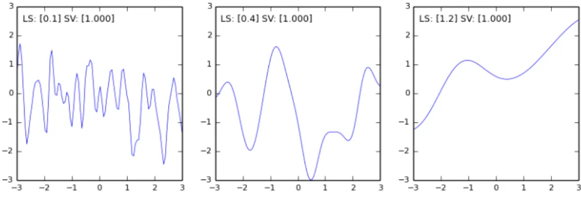
The following figures are examples of random samples drawn from a GP prior distribution (no training inputs), with the CovSEiso covariance function and the hyper-parameters (LS and SV) set as indicated above each panel. The samples are each actually for 100 xaxis values evenly spread between −3.0
and+3.0. They axis represents the variance, also ranging from −3.0 to +3.0. The GP has a zero mean-function. The blue curve is a continuous plot line connecting the points.
Figure 2.4: GP Prior Samples Drawn from a Squared Exponential Kernel - Example 2.
As can be seen from these plots, the prior covariances are controlled by the hyper-parameters. The CovSEiso kernel is a good general purpose kernel and is useful for a first attempt to get a sense of the structure in the data. It is however, often too “smooth” for some applications.
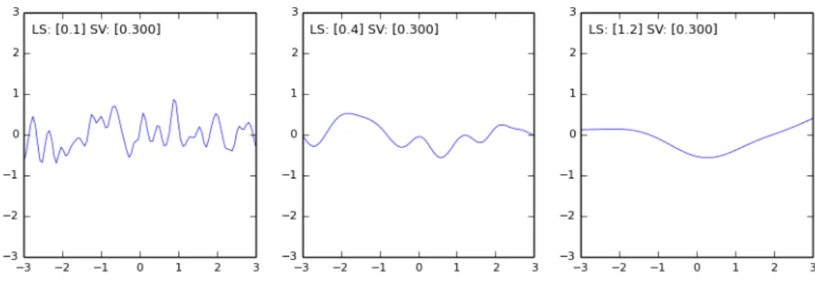
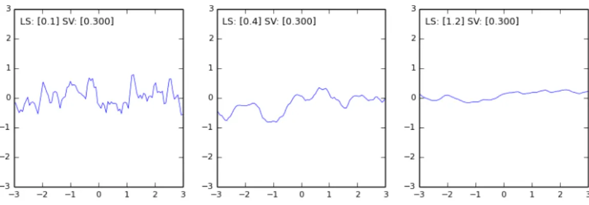
Mat´ern Kernel
The Mat´ern kernel has more flexibility in specifying the “roughness” of the covariances. It is represented by: cM at(xi, xj) =σv2 1 Γ(V)2V−1 2 √ V r l BV 2 √ V r l (2.24)
where the hyper-parameters are alsol, theeffective length scale(LS) andσv2, thesignal variance(SV).
Γ() is the standard Gamma function and B() a modified Bessel function [Rasmussen and Williams
2006]. V is aclassparameter which when constrained to half-integer valuesV = 1/2,3/2,5/2,7/2, provides kernels with increasing degrees of differentiability. Our implementation treats these as different classes of Mat´ern covariance functions by instantiation with a suitable constructor parameter.
Generally,V = 3/2is utilised as it is well suited for rougher models than the SE kernel.
Figure 2.6: GP Prior Samples Drawn from a Mat´ern Kernel - Example 2.
Figures 2.5 and 2.6 show the rougher covariance effects.
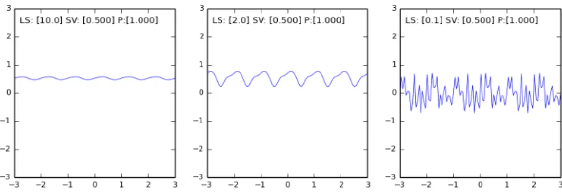
Periodic Kernel
A general Periodic kernel (CovPeriodic) provides for periodicity in the covariance influences between points. It is represented by:
cP er(xi, xj) =σ2vexp −2 l2sin 2 πr p (2.25)
where the hyper-parameters arel, theeffective length scale(LS),σv2, thesignal variance(SV) andpis the period (P). The length scale in this case is relative to the period and for larger values ofl, the effects become sinusoidal, while for small values ofl, the effects are of more complex harmonics.
Figure 2.8: GP Prior Samples Drawn from a Periodic Kernel - Example 2.
Figures 2.7 and 2.8 show the periodic covariance effects. In each case the period is1.0with the varying length scale showing the sinusoidal and more complex harmonics effects. The signal variance affects the amplitude.
Composite Kernels
Composite kernels can be formed by summing two kernels, or taking the product of two kernels, and in each case the resultant kernel is positive semi-definite (PSD) and is thus a valid covariance kernel. We can also then form more complex kernels from combinations of products and sums of kernels.
For this dissertation, in Chapters 4 and 5 we sum the Mat´ern and Periodic kernels in order to discern reasonably complex periodic structure in the MISR-HR data.
Generally, when using covariance kernels, it is often difficult to choose appropriate hyper-parameters and the process of hyper-parameter optimisation or “learning” is required.
2.4.6 GP Hyper-Parameter Learning
In section 2.4.2, equation 2.9 for the negative log likelihood (NLL) was used for measuring the likeli-hood of the predictions. This can also be used for optimisation of the hyper-parameters for a GP model. This is the basic procedure for learning in Gaussian Processes, although much more sophisticated full Bayesian learning methods are provided in [Rasmussen and Williams 2006], along with various alterna-tive approaches. There is also a substantial body of other research work dealing with this topic.
For purposes of this dissertation optimisation is based on the method of determining the hyper-parameters that minimise the NLL, with equation 2.9 as the objective function.
Minimisation is performed using a non-linear optimisation library, in this case NLopt [Johnson]. The COBYLA (Constrained Optimization BY Linear Approximations) algorithm from the NLopt library is used for derivative-free optimisation [Powell 1994] and [Powell 1998].
The (Julia) covariance kernel functions developed or ported for this project have also catered for comput-ing derivatives for hyper-parameters for the CovSEiso, CovMatern and CovPeriodic kernels. A gradient-descent algorithm Low-storage BFGS (L-BFGS), also provided by the NLopt package has also been utilised [Nocedal 1980] and [Liu and Nocedal 1989]. The results of the two optimisation algorithms are similar, with the gradient-descent method being more computationally efficient. The derivative-free method however, is more flexible in handling composite kernels without the complexity of determining derivatives for multiple combinations of kernels.
2.4.7 Gaussian Process Algorithms Toolkit
A comprehensive toolkit, developed in Matlab/Octave, with many of the algorithms described in [Ras-mussen and Williams 2006] and [Nickisch and Ras[Ras-mussen 2008], is described in [Ras[Ras-mussen and Nick-isch 2010] and is available through their companion web site [The Gaussian Process Web Site].
This toolkit was invaluable in learning about Gaussian Processes and for testing various functions. How-ever, it was decided that the Julia language would be used for implementing the GP software components used for this dissertation project.
2.5
Software Components and Libraries
The software components developed for this dissertation are described in this section. These include software functions for MISR-HR data extracts and processing, for Gaussian Process model processing and for plotting.
Although there are many software libraries and tools available which could have been used for many of the data processing and computational requirements for this project, it was decided to primarily use the more recently released (March 2012) Julia Scientific and Technical programming platform [Bezansonet al.2012a].
The key reasons were:
• Gaussian Processes have not previously been implemented in Julia (as at the time of completing this dissertation), and a contribution could thus be made by doing so
• Julia has not been used for data and computational processing for the MISR-HR system, or as far as we know for satellite remote sensing applications generally, and a contribution could also be made in this arena
• Julia has a permissive Open Source license and any software developed for this project could be open-sourced and benefit wider communities
• Julia has an appealing proposition regarding its performance, ease-of-use for scientific applica-tions and its ability to integrate well with other libraries
2.5.1 The Julia Scientific and Technical Programming Platform
The Julia language has been designed [Bezansonet al.2012a] as a programming platform specifically for scientific and technical computing. It is positioned as a high-performance language, fully compiled with similar performance to C++, but with a high-level syntax and the ease of use of similar languages such as R, Python, Matlab and Octave. It also has many of the existing supporting libraries needed for scientific programming and many new ones exploiting modern computing capabilities such as concurrency across processor cores and computing clusters. The Julia web site is at [Bezansonet al.2012b].
In [Lubin and Dunning 2013], Julia was used for implementing a new Algebraic Modelling Language (AML) for use in operations research and optimisation. Benchmarks were carried out for dense and sparse matrix computations used in their algorithms, comparing Julia with implementations in C++, MatLab, PyPy and Python. For these particular benchmarks, Julia’s timed performance was within a factor of 2 of C++, compared with between 4 and 18 of C++ for PyPy and MatLab. Standard Python was 70 times that of C++.