Quantum Algorithm for Finding the Optimal Variable Ordering for Binary Decision Diagrams

Variable Ordering for Binary Decision Diagrams

Seiichiro Tani

NTT Communication Science Laboratories, NTT Corporation, Atsugi, Japan [email protected]

Abstract

An ordered binary decision diagram (OBDD) is a directed acyclic graph that represents a Boolean function. Since OBDDs have many nice properties as data structures, they have been extensively studied for decades in both theoretical and practical fields, such as VLSI (Very Large Scale Integration) design, formal verification, machine learning, and combinatorial problems. Arguably, the most crucial problem in using OBDDs is that they may vary exponentially in size depending on their variable ordering (i.e., the order in which the variables are to be read) when they represent the same function. Indeed, it is NP hard to find an optimal variable ordering that minimizes an OBDD for a given function. Friedman and Supowit provided a clever deterministic algorithm with time/space complexityO∗(3n), wherenis the number of variables of the function, which is much better than the trivial brute-force boundO∗(n!2n). This paper shows that a further speedup is possible with quantum computers by presenting a quantum algorithm that produces a minimum OBDD together with the corresponding variable ordering inO∗(2.77286n) time and space with an exponentially small error probability. Moreover, this algorithm can be adapted to constructing other minimum decision diagrams such as zero-suppressed BDDs.

2012 ACM Subject Classification Theory of computation→Quantum computation theory; Theory of computation→Data structures design and analysis

Keywords and phrases Binary Decision Diagram, Variable Ordering, Quantum Algorithm

Digital Object Identifier 10.4230/LIPIcs.SWAT.2020.36

Related Version A full version of the paper is available athttps://arxiv.org/abs/1909.12658.

1

Introduction

1.1

Background

Ordered binary decision diagrams

The ordered binary decision diagram (OBDD) is one of the data structures that have been most often used for decades to represent Boolean functions in practical situations, such as VLSI design, formal verification, optimization of combinatorial problems, and machine learning, and it has been extensively studied from both theoretical and practical standpoints (see standard textbooks and surveys, e.g., Refs. [8, 12, 7]). Moreover, many variants of OBDDs have been invented to more efficiently represent data with properties observed frequently in specific applications. More technically speaking, OBDDs are directed acyclic graphs that represent Boolean functions and also known as special cases of oblivious read-once branching programs in the field of complexity theory. The reason for OBDDs’ popularity lies in their nice properties – they can be uniquely determined up to isomorphism for each function oncevariable ordering(i.e., the order in which to read the variables) is fixed and, thanks to this property, the equivalence of functions can be checked by just testing the isomorphism between the OBDDs representing the functions. In addition, binary operations such asAND

and_ORbetween two functions can be performed efficiently over the OBDDs representing those functions [2]. Since these properties are essential in many applications, OBDDs

© Seiichiro Tani;

licensed under Creative Commons License CC-BY

have gathered much attention from various research fields. To enjoy these nice properties, however, we actually need to address a crucial problem, which is that OBDDs may vary exponentially in size depending on their variable ordering. For instance, a Boolean function f(x1, . . . , x2n) =x1x2+x3x4+· · ·+x2n−1x2n has a (2n+ 2)-sized OBDD for the ordering (x1, . . . , x2n) and a 2n+1-sized OBDD for the ordering (x1, x3, . . . , x2n−1, x2, x4, . . . , x2n) [8, Sec. 8.1] (see Figure 1 for the case wheren= 6). This is not a rare phenomenon; it could happen in many concrete functions that one encounters. Thus, since the early stages of OBDD research, one of the most central problems has been how to find an optimal variable ordering, i.e., one that minimizes OBDDs. Since there aren! permutations overnvariables, the brute-force search requires at least n! = 2Ω(nlogn) _{time to find an optimal variable} ordering. Indeed, finding an optimal variable ordering for a given function is an NP hard problem (see a short survey in the full paper [11]).

To tackle this high complexity, many heuristics have been proposed to find an optimal variable ordering or a relatively good one. These heuristics work well for Boolean functions appearing in specific applications since they are based on very insightful observations, but they do not guarantee a worst-case time complexity lower than that achievable with the brute-force search. The only algorithm with a much lower worst-case time complexity bound, O∗(3n) time (O∗(·) hides a polynomial factor), than the brute-force boundO∗(n!2n) forall Boolean functions withnvariables was provided by Friedman and Supowit [5], and that was almost thirty years ago!

1.2

Our Results

In this paper, we show that quantum speedup is possible for the problem of finding an optimal variable ordering of the OBDD for a given function. This is the first quantum speedup for the OBDD-related problems. Our algorithms assume the quantum random access memory (QRAM) model [6], which is commonly used in the literature concerned with quantum algorithms. In the model, one can read contents from or write them into quantum memory in a superposition. We provide our main result in the following theorem.

ITheorem 1. There exists a quantum algorithm that, for a functionf:{0,1}n _{→ {0,1}given} as its truth table, produces a minimum OBDD representing f together with the corresponding variable ordering inO∗(γn_{)time and space with an exponentially small error probability with} respect to n, where the constant γ is at most 2.77286. Moreover, the OBDD produced by our algorithm is always a valid one forf, although it is not minimum with an exponentially small probability.

This improves upon the classical best boundO∗₍₃n_{) [5] on time/space complexity. The} classical algorithm achieving this bound is a deterministic one. However, there are no randomized algorithms that compute an optimal variable ordering in asymptotically less time complexity as far as we know.

It may seem somewhat restricted to assume that the function f is given as its truth table, since there are other common representations of Boolean functions such as DNFs, CNFs, Boolean circuits and OBDDs. However, this is not the case. Our algorithm actually works in more general settings where the input functionf is given as any representation such that the value off on any specified assignment can be computed over the representation in polynomial time inn, such as polynomial-size DNFs/CNFs/circuits and OBDDs of any size. This is because, in such cases, the truth table off can be prepared inO∗(2n) time and the minimum OBDD is computable from that truth table with our algorithm. We restate Theorem 1 in a more general form as follows.

ICorollary 2. LetR(f)be any representation of a Boolean functionf withnvariables such that the value of f(x) on any given assignment x∈ {0,1}n _{can be computed on R(f) in} polynomial time with respect ton. Then, there exists a quantum algorithm that, for a function f:{0,1}n_{→ {0,1} given asR(f), produces a minimum OBDD representing f together with} the corresponding variable ordering inO∗(γn_{)time and space with an exponentially small error} probability with respect ton, where the constantγis at most2.77286. Possible representations asR(f)are polynomial-size DNFs/CNFs/circuits and OBDDs of any size for function f.

There are many variants of OBDDs, among which the zero-suppressed BDDs (ZDDs or ZBDDs) introduced by Minato [9] have been shown to be very powerful in dealing with combinatorial problems (see Knuth’s famous book [7] for how to apply ZDDs to such problems). With slight modifications, our algorithm can construct a minimum ZDD with the same time/space complexity. We believe that similar speedups are possible for many other variants of OBDDs (adapting our algorithm to multiterminal BDDs (MTBDDs) [8] is almost trivial).

Technical Contribution

Recently, Ambainis et al. [1] has introduced break-through quantum techniques to speed up classical dynamic programming approaches. Inspired by their technique, our quantum algorithm speeds up the classical one (calledFS) discovered by Friedman and Supowit [5]. Ambainis et al.’s results depend on the property that a large problem can be divided into subproblems that can be regarded as a scale-down version of the original problem and can be solved with the same algorithm, as is often the case with graph problems. In our case, firstly, it is unclear whether the problem can be divided into subproblems. Secondly, subproblems would be to optimize the ordering of variables starting from the middle variable or even from the opposite end, i.e., from the variable to be readfirst, toward the one to be readlast. Such subproblems cannot be solved with the algorithmFS, and, in particular, optimizing in the latter case essentially requires the equivalence check of subfunctions off, which is very costly. Our technical contribution is to find, by carefully observing the unique properties of OBDDs, that it is actually possible to even recursively divide the original problem into not the same but somewhat similar kinds of subproblems, to generalize the algorithmFSso that it can solve the subproblems, and to use the quantum minimum finding algorithm to efficiently select the subproblems that essentially contribute to the optimal variable ordering. In the full paper [11], we provide the technical outline of our algorithm, which would help readers understand the structure of our algorithm.

2

Preliminaries

2.1

Basic Terminology

LetN,ZandRbe the sets of natural numbers, integers, and real numbers, respectively. For eachn∈N, let [n] be the set{1, . . . , n}, andSn be the permutation group over [n]. We may denote a singleton set{k} bykfor notational simplicity if it is clear from the context; for instance,I\ {k}may be denoted byI\k, if we knowI is a set. For any subsetI⊆[n], let Πn(I) be the set ofπ∈ Sn such that the first|I|members {π[1], . . . , π[|I|]} constitutesI, i.e.,

For simplicity, we omit the subscriptnand write Π(I). More generally, for any two disjoint subsetsI, J ⊆[n], let

Πn(hI, Ji) :={π∈ Sn: {π[1], . . . , π[|I|]}=I,{π[|I|+ 1], . . . , π[|I|+|J|]}=J} ⊆ Sn. For any disjoint subsetsI1, . . . , Im⊆[n] form∈[n], Πn(hI1, . . . , Imi) is defined similarly. For simplicity, we may denotehIibyI, if it is clear from the context.

We denote the union operation overdisjoint sets byt(instead of∪) when we emphasize the disjointness of the sets.

For nBoolean variablesx1, . . . , xn, any set I⊆[n], and any vectorb= (b1, . . . , b|I|)∈ {0,1}|I|_{, xI denotes the ordered set (xj}

1, . . . , xj|I|), where {j1, . . . , j|I|} = I and j1 < · · · < j_|I|, and xI = b denotes xji = bi for each i = [|I|]. For any Boolean function

f:{0,1}n_{→ {0,1} with variablesx}

1, . . . , xn, we denote byf|xI=b the function obtained by

restrictingf withxI =b. IfIis a singleton set, say,I={i}, we may writexi andf|xi=b to

meanx{i} andf|x{i}=b, respectively, for notational simplicity. We say thatg is asubfunction off ifg is equivalent to the functionf|xI=b for some I⊆[n] andb∈ {0,1}

|I|_.

For any functiong(n) inn, we use the notationO∗(g(n)) to hide a polynomial factor in n. We further denoteX=O∗(Y) byX _/Y.

We use the following upper bound many times in this paper. Forn∈Nandk∈[n]∪ {0}, it holds that n_k

≤2nH(k/n)_{, whereH(·) represents the binary entropy function H(δ) :=} −δlog₂δ−(1−δ) log₂(1−δ).

2.2

Ordered Binary Decision Diagrams

We provide a quick review of OBDDs. For more details, consult standard textbooks (e.g., Refs. [8, 12]).

For any Boolean functionf:{0,1}n_{→ {0,1}over variablesx}

1, . . . , xn and any permuta-tionπ∈ Sn (called avariable ordering), an OBDD B(f, π) is a single-rooted directed acyclic graphG(V, E) that is unique up to isomorphism, defined as follows (examples are shown in Figure 1).

1. The node setV is the union of two disjoint setsN andT ofnon-terminal nodes with out-degree two andterminal nodes with out-degree zero, respectively, whereT contains exactly two nodes: T ={f,t}. The setN contains a unique source noder, called theroot.

2. B(f, π) is a leveled graph with n+ 1 levels. Namely, the node set can be partitioned intonsubsets: V :=V0tV1t · · · tVn,whereVn={r} andV0=T ={t,f}, such that each directed edge (u, v)∈E is in Vi×Vj for a pair (i, j)∈[n]×({0} t[n−1]) with i > j. For eachi∈[n], subsetVi (called theleveli) is associated with the variablexπ[i], or alternatively, each node inVi is labeled withxπ[i].1 For convenience, we define a map var:N →[n] such that ifv∈Vi thenvar=π[i].

3. The two edges emanating from every non-terminal nodev are called the 0-edgeand the 1-edge, which are labeled with 0 and 1, respectively. For everyu∈N, letu0 andu1be the destinations of the 0-edge and 1-edge ofu, respectively.

4. Let F(f) be the set of all subfunctions off. Define a bijective mapF:V → F(f) as follows: (a)F(r) =f for r∈Vn; (b) F(t) =trueandF(f) =falsefort,f∈V0; (c) For everyu∈N andb∈ {0,1},F(ub) is the subfunction obtained fromF(u) by substituting xvar(u) withb, i.e., F(ub) =F(u)|xvar(u)=b.

1 _{In the standard definition,V}

iis associated with the variablexπ[n−i]. Our definition follows the one

𝑥" 𝑥# 𝑥$ 𝑥% 𝑥& 𝑥' T F 𝑥" 𝑥$ 𝑥$

𝑥& 𝑥& 𝑥& 𝑥&

𝑥# 𝑥# 𝑥# 𝑥# 𝑥% 𝑥% 𝑥' T F 𝑉) 𝑉' 𝑉& 𝑉% 𝑉$ 𝑉# 𝑉"

Figure 1The OBDDs represent the functionf(x1, x2, x3, x4, x5, x6) =x1x2+x3x4+x5x6 under two variable orderings: (x1, x2, x3, x4, x5, x6) (left) and (x1, x3, x5, x2, x4, x6) (right), where the solid and dotted arcs express 1-edges and 0-edges, respectively, and the terminal nodes fortrue

andfalseare labeled with TandF, respectively. For eachn∈N, the functionf(x1, . . . , x2n) =

x1x2+x3x4+· · ·+x2n−1x2n has a (2n+ 2)-sized OBDD for the ordering (x1, . . . , x2n) and a 2n+1_{-sized OBDD for the ordering (x}

1, x3, . . . , x2n−1, x2, x4, . . . , x2n).

5. B(f, π) must be minimal in the sense that the following reduction rules cannot be applied. In other words,B(f, π) is obtained by maximally applying the following rules:

a. if there exists a redundant nodeu∈N, then removeuand its outgoing edges, and redirect all the incoming edges of utou0, where a nodeuis redundant ifu0 is the same node asu1.

b. if there existequivalent nodes{u, v} ⊂N, then removev(i.e., any one of them) and its outgoing edges, and redirect all incoming edges ofv tou, whereuandv are equivalent if (1) var(u) is equal tovar(v), and (2) u0 andu1 are the same nodes as v0 andv1, respectively.

For eachj ∈[n],Costj(f, π) denotes the width at the level associated with the variable xj, namely, the number of nodes in the levelπ−1[j] (see Figure 2 in Appendix). ForI⊆[n], letπI be a permutationπin Π(I) that minimizes the number of nodes in level 1 to level|I|:

πI := arg min

   |I| X j=1 Costπ[j](f, π) :π∈Π(I)    . (1)

Note that P|I|

j=1Costπ[j](f, π) =Pi∈ICosti(f, π) forπ∈Π(I). More generally, for disjoint subsetsI1, . . . , Im⊆[n],πhI1,...,Imiis a permutation in Π(hI1, . . . , Imi) that minimizes the

number of the nodes in level 1 to level|I1|+· · ·+|Im|over allπ∈Π(hI1, . . . , Imi):

π_hI1,...,Imi:= arg min    |I1|+···+|Im| X j=1 Costπ[j](f, π) :π∈Π(hI1, . . . , Imi)    . (2)

Note that minP|I1|+···+|Im|

j=1 Costπ[j](f, π) =

P

i∈I1t···tImCosti(f, π) for anyπ∈Π(hI1, . . . , Imi).

The following well-known lemma captures the essential property of OBDDs. It states that the number of nodes at level i ∈ [n] is constant over all π, provided that the two sets {π[1], . . . , π[i−1]}and{π[i+ 1], . . . , π[n]}are fixed (see Figure 3 in Appendix).

ILemma 3([5]). For any non-empty subsetI⊆[n] and anyi∈I, there exists a constant cf such that, for each π∈Π(hI\ {i},{i}i),Costπ[|I|](f, π)≡Costi(f, π) =cf.

For convenience, we define shorthand for the minimums of the sums in Eqs. (1) and (2). ForI0 ⊆I ⊆[n], _mincostI[I0] is defined as the number of nodes in the levels associated with variables indexed by elements inI0 under permutationπI, namely, mincostI[I0] :=

P

i∈I0Costi(f, πI).More generally, for disjoint subsetsI1, . . . , Im⊆[n] andI0⊆I1t · · · tIm,

mincosthI1,...,Imi[I

0_{] :=}X

i∈I0

Costi(f, πhI1,...,Imi).

As a special case, we denote_mincosthI1,...,Imi[I1t · · · tIm] bymincosthI1,...,Imi. We define

mincost∅ as 0.

2.3

The Algorithm by Friedman and Supowit

This subsection reviews the algorithm by Friedman and Supowit [5]. We will generalize their idea later and heavily use the generalized form in our quantum algorithm. Hereafter, we call their algorithmFS.

2.3.1

Key Lemma and Data Structures

The following lemma is the basis of the dynamic programming approach used inFS. ILemma 4. For any non-empty subsetI⊆[n]and any Boolean functionf: {0,1}n_{→ {0,1},} the following holds:

mincostI = mink∈I mincostI\k+Costk(f, πhI\k,ki)

= mink∈I mincosthI\k,ki

. The proof is given in the full paper [11].

Before sketching algorithmFS, we provide several definitions. For anyI⊆[n],_tableI is an array with 2n−|I| cells each of which stores a non-negative integer. Intuitively, for b∈ {0,1}n−|I|_{, the cell}

tableI[b] stores (the pointer to) the unique node ofB(f, πI) associated viaF with functionf|x_[n]\I=b. Hence, we may writetableI[x[n]\I =b] instead oftableI[b] to clearly indicate the value assigned to each variable xj for j ∈[n]\I. The purpose of

tableI is to relate all subfunctionsf|x[n]\I=b (b∈ {0,1}

n−|I|_{) to the corresponding nodes of} B(f, πI). We assume without loss of generality that the pointers to nodes ofB(f, πI) are non-negative integers and, in particular, those to the two terminal nodes corresponding to falseandtrueare the integers 0 and 1, respectively. Thus,table∅ is merely the truth table off.

AlgorithmFScomputestableI together withπI,mincostI, and another data structure,

nodeI for allI⊆[n], starting fromtable∅ via dynamic programming. nodeI is the set of all triples of (the pointers to) nodes, (u, u0, u1)∈N×(NtT)×(NtT), inB(f, πI), where var(u) =πI[|I|], and (u, u0) and (u, u1) are the 0-edge and 1-edge ofu, respectively. Thus,

nodeI contains the structure of the subgraph ofB(f, πI) induced byV|I|. The purpose of thenodeI is to prevent the algorithm from duplicating existing nodes, i.e., creating nodes associated with the same subfunctions as those with which the existing nodes are associated. By the definition,node∅ is the empty set. We assume thatnodeI is implemented with an appropriate data structure, such as a balanced tree, so that the time complexity required for membership testing and insertion is the order of logarithm in the number of triples stored in

More generally, for disjoint subset I1, . . . , Im ⊆ [n], tablehI1,...,Imi is an array with

2n−|I1t···tIm|_{cells such that, for b∈ {0,1}}n−|I1t···tIm|_{, table}

hI1,...,Imi[b] stores the nodes

of B(f, π_hI1,...,Imi) associated with the functionf|x[n]\I1t···tIm=b. nodehI1,...,Imi is defined

similarly for B(f, πhI1,...,Imi). For simplicity, we hereafter denote byF S(hI1, . . . , Imi) the

quadruplet (πhI1,...,Imi,mincosthI1,...,Imi,tablehI1,...,Imi,nodehI1,...,Imi).

2.3.2

Sketch of Algorithm FS

Algorithm FSperforms the following operations for k = 1, . . . , n in this order. For each k-element subsetI⊆[n], computeF S(hI\i, ii) fromF S(hI\ii) for eachi∈Iin the manner described later (note that, since the cardinality of the set I\i is k−1, F S(hI\ii) has already been computed). Then setF S(I)←− F S(hI\i∗_{, i}∗_i),wherei∗ _{is the indexi∈I} that minimizesmincosthI\i,ii, implying thatπI isπhI\i∗_,i∗_i. This is justified by Lemma 4. A schematic view of the algorithm is shown in Figure 5 in Appendix.

To compute F S(hI\i, ii) fromF S(hI\ii), do the following. First set_nodehI\i,ii← ∅ andmincosthI\i,ii←mincostI\i as their initial values. Then, for eachb∈ {0,1}n−|I|, set

u0←tableI\i[x[n]\I =b, xi= 0], u1←tableI\i[x[n]\I =b, xi= 1].

Ifu0=u1, then storeu0 intablehI\i,ii[b]. Otherwise, test whether (u, u0, u1) for someuis a member of_nodeI\i. If it is, storeuin thetablehI\i,ii[b]; otherwise create a new triple (u0_{, u}

0, u1), insert it tonodehI\i,iiand incrementmincosthI\i,ii. Sinceu0 is the pointer to the new node, u0 must be different from any pointer already included in nodehI\i,ii and from any pointer to a node inV1t · · · tVk−1 inB(f, πhI\ii), wherek =|I|. Suchu0 can be easily chosen by settingu0 to two plus the value ofmincosthI\i,iibefore the increment, since the_mincosthI\i,iiis exactly the number of triples in nodehI\i,ii plus|V1t · · · tVk−1|, and the numbers 0 and 1 are reserved for the terminal nodes. We call the above procedure table folding with respect toxi, because it halves the size of_tablehI\ii. We also mean it by “foldingtablehI\ii with respect toxi”.

The complexity analysis is fairly simple. For each k, we need to computeF S(I) for n

k

possible I’s with |I| = k. For each I, it takes O∗(2n−k) time since the the size of

tableI\i is 2n−k+1 and each operation to nodeI\i takes a polynomial time in n. Thus, the total time is Pn

k=02n−k +1 n

k

= 2·3n up to a polynomial factor. The point is that computing eachF S(I) takes time linear to the size of_tableI\i up to a polynomial factor. The space required by AlgorithmFSduring the process forkis dominated by that fortableI,

tableI\i andnodeI for allI and i∈I, which is O∗ 2n−k n_k. The space complexity is thusO∗ _max

k∈{0}∪[n]2n−k n_k

=O∗₍₃n_).

ITheorem 5(Friedman and Supowit [5]). Suppose that the truth table off:{0,1}n_{→ {0,1}} is given as input. AlgorithmFSproducesF S([n])in O∗(3n_{)time and space.}

2.4

Quantum Computation

We assume that readers have a basic knowledge of quantum computing (e.g., Ref. [10]). We provide only a lemma used to obtain our results.

ILemma 6 (Quantum Minimum Finding [4, 3]). For every ε >0there exists a quantum algorithm that, for a function f: [N]→Zgiven as an oracle, finds an elementx∈[N]at whichf(x)achieves the minimum, with error probability at mostεby makingO(pNlog(1/ε)) queries.

In this paper, the search space N is exponentially large in nand we are interested in exponential complexities, ignoring polynomial factors in them. We can thus safely assume ε= 1/2p(n)_{for a polynomialp(n), so that the overhead is polynomially bounded. Since our} algorithms use Lemma 6 a constant number of times, their overall error probabilities are exponentially small for a sufficiently largep(n). In the following proofs, we thus assume that εis exponentially small whenever we use Lemma 6, and do not explicitly analyze the error probability for simplicity.

Our algorithms assume the quantum random access memory (QRAM) model [6], which is commonly used in the literature when considering quantum algorithms. In the model, one can read contents from or write them into quantum memory in a superposition.

3

Quantum Algorithm with Divide-and-Conquer

We generalize Lemma 4 and Theorem 5 and use them in our quantum algorithm.

I Lemma 7. For any disjoint subsets I1, . . . , Im, J ⊆ [n] with J 6= ∅ and any Boolean functionf:{0,1}n_{→ {0,1}, the following holds:}

mincosthI1,...,Im,Ji= min

k∈J mincosthI1,...,Im,J\{k}i+Costk(f, πhI1,...,Im,J\{k},{k}i)

= min

k∈J mincosthI1,...,Im,J\{k},{k}i

.

The proof of this lemma is very similar to that of Lemma 4 and given in the full paper [11]. Based on Lemma 7, we generalize Theorem 5 to obtain algorithmFS∗ (its pseudo code is given below, and a schematic view ofFS∗ is shown in Figure 6 in Appendix).

ILemma 8 (Classical Composition Lemma). For disjoint subsetsI1, . . . , Im, J ⊆[n] with J 6=∅, there exists a deterministic algorithm FS∗ that producesF S(hI1, . . . , Im, Ji) from F S(hI1, . . . , Imi)for an underlying functionf:{0,1}n→ {0,1}inO∗ 2n−|I1t···tImtJ|·3|J| time and space. More generally, for eachk∈[|J|], the algorithm produces the set{F S(hI1, . . . ,

Im, Ki) :K⊆J,|K|=k} from F S(hI1, . . . , Imi) in O∗

2n−|I1t···tImtJ|Pk j=02|J|−j |J| j

time and space.

Note that ifI1t · · · tIm=∅andJ = [n], then we obtain Theorem 5.

Proof. We focuses on the simplest case ofm= 1, for which our goal is to show an algorithm that producesF S(hI, Ji) fromF S(I). It is straightforward to generalize the proof to the case ofm≥2. Starting fromF S(I), the algorithm first folds_tableI with respect to each variable in {xj: j ∈ J} to obtain F S(hI, ji) for every j ∈ J, then fold tablehI,j1i with

respect toxj₂ andtablehI,j2i with respect toxj1 to obtainF S(hI,{j1, j2}i) by taking the

minimum of_mincosthI,j1,j2i andmincosthI,j2,j1i for every j1, j2 ∈J, and repeat this to

finally obtainF S(hI, Ji). This algorithms is justified by Lemma 7. For eachj∈[|J|],K⊆J with|K|=j, andh∈K, the time complexity of computingF S(hI, Ki) fromF S(hI, K−hi) is linear to the size oftablehI,Ki, i.e., 2n−|I|−j up to a polynomial factor. The total time is thus, up to a polynomial factor,

|J| X j=1 2n−|I|−j |J| j <2n−|I|−|J| |J| X j=0 2|J|−j |J| j = 2n−|ItJ|·3|J|.

If we stop the algorithm atj =k, then the algorithm produces the set{F S(hI, Ki) :K⊆ J,|K|=k}. The time complexity in this case is at most 2n−|I|−|J|Pk

j=02 |J|−j |J| j , up to a polynomial factor.

Since the space complexity is trivially upper-bounded by the time complexity, we complete

the proof. _J

IRemark 9. It is not difficult to see that the algorithmFS∗ works even when the functionf has a multivalued function: f:{0,1}n _{→Z. The only difference from the Boolean case is that} the truth table maps each Boolean assignment to a value inZ. In this case, the algorithm produces a variant of an OBDD (called a multi-terminal BDD, MTBDD) of minimum size. In addition, our algorithm with slight modifications to the table folding rule in FS∗ can construct a minimum zero-suppressed BDD (ZDD) [9] for a given Boolean function. The details are described in the full paper [11]. These modifications are also possible for the quantum algorithms described later, since they perform table folding by runningFS∗ as a subroutine.

Algorithm FS∗Composable variant of algorithmFS. “A←B” means thatBis substituted forA.

Input: disjoint subsetsI, J∈[n] andF S(I)

Output: F S(hI, Ji)

1 FunctionMain()

2 for`:= 1to|J|do

3 foreach`-element subsetK⊆Jdo

4 _mincosthI,Ki←+∞; // init.

5 foreachk∈Kdo

6 F S(hI, K\k, ki)←FOLD(I, K, k,F S(hI, K\ki)); 7 if _mincosthI,Ki>mincosthI,K\k,kithen

8 F S(hI, Ki)← F S(hI, K\k, ki); 9 end 10 end 11 end 12 end 13 returnF S(hI, Ji) 14 end

15 FunctionFOLD(I, K, k,F S(hI, K\ki)) // produce F S(hI, K\k, ki) from F S(hI, K\ki)

16 πhI,K\k,ki∈ {π∈Π(hI, K\k, ki) :π[i] =πhI,K\ki[i] (i= 1, . . . ,|ItK| −1)}; // init. 17 _mincosthI,K\k,ki←mincosthI,K\ki; // init.

18 _nodehI, K\k, ki ← ∅; // init. 19 forb∈ {0,1}n−|I|−|K| do 20 u0←tablehI,K\ki[x[n]\(ItK)=b, xk= 0]; 21 u1←tablehI,K\ki[x[n]\(ItK)=b, xk= 1]; 22 if u0=u1 then 23 _tablehI,K\k,ki[x[n]\(ItK)=b]←u0 24 else if ∃u(u, u0, u1)∈nodehI, K\k, kithen 25 _tablehI,K\k,ki[x[n]\(ItK)=b]←u

26 else // create a new node

27 u←_mincosthI,K\k,ki+ 2;

28 _tablehI,K\k,ki[x[n]\(ItK)=b]←u; 29 _mincosthI,K\k,ki←mincosthI,K\k,ki+ 1; 30 insert (u, u0, u1) intonodehI, K\k, ki

31 end

32 end

33 returnF S(hI, K\k, ki) 34 end

The following theorem is the basis of our quantum algorithms.

ILemma 10 (Divide-and-Conquer). For any disjoint subsets I1, . . . , Im, J ⊆[n]with J 6=∅ and any k∈[|J|], it holds that _mincosthI1,...,Im,Ji[J] is equal to

min

K:K⊆J,|K|=k mincosthI1,...,Im,Ki

[K] +_mincosthI1,...,Im,K,J\Ki[J\K]

. (3)

In particular, whenI1t · · · tIm=∅ andJ = [n], it holds that

mincost[n]= min

K⊆[n],|K|=k mincostK+mincosthK,[n]\Ki[[n]\K]

. (4)

Proof. We first prove the special case ofI1t · · · tIm=∅ andJ = [n]. By the definition, we have mincost[n]= n X j=1 Costπ[j](f, π) = k X j=1 Costπ[j](f, π) + n X j=k+1 Costπ[j](f, π)

for the optimal permutation π = π[n]. Let K = {π[1], . . . , π[k]}. By Lemma 3, the first sum is independent of how π maps {k+ 1, . . . , n} to [n]\K. Thus, it is equal to the minimum ofPk

j=1Costπ1[j](f, π) over allπ1 ∈ Π(K), i.e., mincostK. Similarly, the

second sum is independent of howπ maps [k] to K. Thus, it is equal to the minimum of

Pn

j=k+1Costπ2[j](f, π) over all π2 ∈ Π(hK,[n]\Ki), i.e., mincosthK,[n]\Ki[[n]\K]. This

completes the proof of Eq. (4).

We can generalize this in a straightforward manner. Let π = πhI1,...,Im,Ji and ` =

|I1t · · · tIm|. Then, we have

mincosthI1,...,Im,Ji[J] =

k X j=1 Costπ[`+j](f, π) + |J| X j=k+1 Costπ[`+j](f, π).

By definingK:={π[`+1], . . . , π[`+k]}, the same argument as the special case of`= 0 implies that the first and second sums are_mincosthI1,...,Im,Ki[K] andmincosthI1,...,Im,K,J\Ki[J\K],

respectively. This completes the proof of Eq. (3). _J A schematic view of the above lemma is shown in Figure 7 in Appendix.

3.1

Simple Cases

We provide simple quantum algorithms on the basis of Lemma 10. The lemma states that, for anyk∈[n],mincost[n] is the minimum ofmincostK+mincosthK,[n]\Ki[[n]\K] over all K ⊆[n] with |K| = k. To find K from among n_k

possibilities that minimizes this amount, we use the quantum minimum finding (Lemma 6). To computemincostK+

mincosthK,[n]\Ki[[n]\K] =mincosthK,[n]\Ki, it suffices to first computeF S(K) (including

mincostK), and thenF S(hK,[n]\Ki) (includingmincosthK,[n]\Ki) fromF S(K). The time complexity for computingF S(K) fromF S(∅) isO∗(2n−k3k_{) by Lemma 8 withI}

1t· · ·tIm=∅ and J = K, while that for computing F S(hK,[n]\Ki) from F S(K) is O∗(3n−k) by Lemma 8 withm= 1,I1=K, andJ = [n]\K. Thus, the time complexity for computing F S(hK,[n]\Ki) from F S(∅) isO∗(2n−k3k_{+ 3}n−k_{). Thus, fork=αnwithα∈[0,1] fixed} later, the total time complexity up to a polynomial factor is

T(n) = s n αn 2(1−α)n3αn+ 3(1−α)n≤212H(α)n n 2[(1−α)+αlog23]n_{+ 2}[(1−α) log23]n o .

To balance the both terms, we set (1−α) +αlog23 = (1−α) log23 and obtain α=α∗, whereα∗= log23−1 2 log₂3−1 ≈0.269577.We have min α∈[0,1]T(n) =O 212H(α ∗_)n+(1−α∗_)n+α∗_(log 23)n =O(γ₀n),

whereγ0 = 2.98581. . .. 2 This slightly improves the classical best boundO∗(3n) on the time complexity. To improve the bound further, we introduce a preprocess that classically computes F S(K) for every K with |K| = αn (α ∈ (0,1)) by using Algorithm FS∗. By Lemma 8, the preprocessing time is then

αn X j=1 2n−j· _n j ≤αn· max j∈[αn]2 n−j _n j / 2(1−α)n+H(α)n (α <1/3) 223n+H(1/3)n (α≥1/3), (5) since 2n−j n_j

increases whenj < n/3 and decreases otherwise. Note that once this preprocess is completed, we can useF S(K) for free and assume that the cost for accessingF S(K) is polynomially bounded for allK⊆[n] with|K|=αn.

Then, assuming that α <1/3, the total time complexity up to a polynomial factor is

T(n) = αn X j=1 2n−j· _n j + s _n αn nO(1)+ 3(1−α)n_/2[(1−α)+H(α)]n+2[12H(α)+(1−α) log23]n_.

To balance the both terms, we set (1−α) +H(α) = ₂1H(α) + (1−α) log23 and obtain the solutionα=α∗, whereα∗ := 0.274863. . ., which is less than 1/3 as we assumed. At α=α∗, we have T(n)_/2[(1−α∗_)+H(α∗_)]n

= O∗(γn

1), where γ1 is at most 2.97625 (< γ0). Thus, introducing the preprocess improves the complexity bound. A schematic view of the above algorithm is shown in Figure 8 in Appendix.

3.2

General Case

We can improve this bound further by applying Lemma 10 ktimes. We denote the resulting algorithm with constant parametersk∈Nandα:= (α1, . . . , αk) byOptOBDD(k,α) where 0< α1 <· · ·< αk <1. Its pseudo code is given below. In addition, we assume α1 <1/3 andαk+1= 1 in the following complexity analysis.

To simplify notations, define two function as follows: for x, y∈(0,1) such that x < y, f(x, y) := 1₂y·H(x/y) +g(x, y) andg(x, y) := (1−y) + (y−x) log₂(3).

By Lemma 8, the time required for the preprocess is Pα1n

`=12 n−`_· n

`

up to a polynomial factor. Thus, the total time complexity can be described as the following recurrence:

T(n) = α1n X `=1 2n−`· _n ` +Lk+1(n), (6) Lj+1(n) = s αj+1n αjn Lj(n) + 2(1−αj+1)n₃(αj+1−αj)n = s _αj +1n αjn Lj(n) + 2g(αj,αj+1)n , (7) 2 _{More precisely,α}∗

must be rounded so thatα∗nis an integer. We assume hereafter for simplicity of

analysis thatnis sufficiently large so that the rounding error is negligible compared to the approximation

Algorithm OptOBDD(k, α) Quantum OBDD-minimization algorithm with constant paramet-ersk∈Nandα:= (α1, . . . , αk)∈[0,1]k satisfying 0< α1<· · ·< αk<1, where the quantum minimum finding algorithm is used in line 8, andFS∗is used in lines 2 and 15. “A←B” means thatBis substituted forA.

Input: F S(∅) :={table∅,π∅,mincost∅,node∅} (accessible from all Functions)

Output: F S([n])

1 FunctionMain()

2 compute the set{F S(K) :K⊆[n], |K|=bα1nc}by algorithmFS(orFS∗); 3 make the set of theseF S(K) global (i.e., accessible from all Functions); 4 returnDivideAndConquer([n], k+ 1)

5 end

6 FunctionDivideAndConquer(L, t) // Compute F S(L) with α1, . . . , αt(=|L|/n)

7 if t= 1then returnF S(L); // F S(L) has been precomputed.

8 FindK(⊂L) of cardinalitybαt−1nc, with Lemma 6, that minimizesmincosthK,L\Ki, 9 which is computed as a component ofF S(hK, L\Ki) by callingComputeFS(K, L\K, t); 10 letK∗be the set that achieves the minimum;

11 returnF S(hK∗, L\K∗i) 12 end

13 FunctionComputeFS(K, M, t) // Compute F S(hK, Mi) with α1, . . . , αt

14 F S(K)←DivideAndConquer(K, t−1);

15 F S(hK, Mi)←FS∗(K, M,F S(K)); 16 returnF S(hK, Mi)

17 end

where j ∈ [k] and L1(n) = O∗(1). Intuitively, Lj(n) is the time required for producing F S(hK1, K2\K1, . . . , Kj\Kj−1i) such thatmincosthK1,K2\K1,...,Kj\Kj−1iis minimum over

allK1, . . . , Kj−1 satisfying|K`|=α`nfor every`∈[k+ 1] andK`⊂K`+1 for every `∈[k]. Since L1(n) = O∗(1), we have L2(n) / q α2n α1n ·2g(α1,α2)n _{/ 2}f(α1,α2)n_{. By setting} f(α1, α2) =g(α2, α3), we haveL3(n) = q α3n α2n ·(L2(n) + 2g(α2,α3)n)/ q α3n α2n ·2g(α2,α3)n_/

2f(α2,α3)n_{.In general, forj= 2, . . . , k, settingf(αj−}

1, αj) =g(αj, αj+1) yields Lj+1(n)/2f(αj,αj+1)n.

Therefore, the total complexity [Eq. (6)] is

T(n)_/ α1n X `=1 2n−`· _n ` + 2f(αk,αk+1)n /2(1−α1)n+H(α1)n_{+ 2}f(αk,1)n_,

where we use α1 <1/3, αk+1 = 1, and Eq. (5). To optimize the right-hand side, we set parameters so that 1−α1+H(α1) =f(αk,1).

In summary, we need to find the values of parametersα1, . . . , αk that satisfy the following system of equations andα1<1/3:

1−α1+H(α1) =f(αk,1), (8)

f(αj−1, αj) =g(αj, αj+1) (j= 2, . . . , k). (9) By numerically solving this system of equations, we obtainT(n) =O(γn

k), whereγkis at most 2.83728 fork= 6. The value ofγk becomes smaller ask increases. However, incrementingk beyond 6 provides only negligible improvement ofγk. Since the space complexity is trivially upper-bounded by the time complexity, we have the following theorem. Note that the values

ofαi’s are not symmetric with respect to 1/2. This reflects the fact that optimizing cost is not symmetric with respect to 1/2, contrasting with many other combinatorial problems. ITheorem 11. There exists a quantum algorithm that, for the truth table off: {0,1}n_→ {0,1} given as input, producesF S([n])with probability 1−exp(−Ω(n)) inO∗(γn_{)time and} space, where the constant γ is at most2.83728, which is achieved by OptOBDD(k,α) with k= 6 andα= (0.183791,0.183802,0.183974,0.186131,0.206480,0.343573).

4

Quantum Algorithm with Composition

4.1

Quantum Composition Lemma

By generalizing the quantum algorithm given in Theorem 11, we now provide a quantum version of Lemma 8, called thequantum composition lemma.

ILemma 12(Quantum Composition: Base Part). For any disjoint subsetsI1, . . . , Im, J⊆[n] withJ 6=∅, there exists a quantum algorithm that, with probability1−exp(−Ω(n)), produces F S(hI1, . . . , Im, Ji)from F S(hI1, . . . , Imi)for an underlying functionf:{0,1}n→ {0,1} in O∗ 2n−|I1t···tImtJ|_·γ|J|_{time and space, where γ is the constant defined in Theorem 11.}

The proof is given in the full paper [11]. The proof idea is similar to that used in the proof of Lemma 8. A pseudo code of the algorithm provided in Lemma 12 is shown below asOptOBDD∗Γ(k,α), where the subroutine Γ appearing in line 17 is set to the deterministic algorithmFS∗, andkandα are set to the values specified in Theorem 11.

Algorithm OptOBDD∗Γ(k, α) Composable Quantum OBDD-minimization algorithm with subroutine Γ and constant parametersk∈Nandα= (α1, . . . , αk)∈[0,1]k satisfying 0< α1< · · ·< αk<1, where the quantum minimum finding algorithm is used in line 9, and subroutine Γ is used in line 17. “A←B” means thatB is substituted forA. Γ(I1, I2, J,F S(I1, I2)) produces F S(hI1, I2, Ji) fromF S(hI1, I2i).

Input: I⊆[n],J⊆[n],F S(I). (accessible from all Functions)

Output: F S(hI, Ji)

1 FunctionMain()

2 n0← |J|; // init.

3 compute the set{F S(hI, Ki) :K⊆J, |K|=bα1n0c}by algorithmFS∗;

4 maken0and the above set ofF S(hI, Ki) global (i.e., accessible from all Functions); 5 returnDivideAndConquer(J, k+ 1)

6 end

7 FunctionDivideAndConquer(L, t) // Compute F S(hI, Li) with α1, . . . , αt

8 if t= 1then returnF S(I, L); // F S(I, L) has been precomputed.

9 FindK(⊂L) of cardinalitybαt−1n0c, with Lemma 6, that minimizesmincosthI,K,L\Ki 10 which is computed as a component ofF S(hI, K, L\Ki)

11 by callingComputeFS(I, K, L\K, t); 12 letK∗be the set that achieves the minimum; 13 returnF S(hI, K∗, L\K∗i)

14 end

15 FunctionComputeFS(I, K, M, t) // Compute F S(hI, K, Mi) with α1, . . . , αt

16 F S(I, K)←DivideAndConquer(K, t−1);

17 F S(hI, K, Mi)←Γ(I, K, M,F S(I, K)); 18 returnF S(hI, K, Mi)

ILemma 13(Quantum Composition: Induction Part). Suppose thatΓis a quantum algorithm that, for any disjoint subsets I1, . . . , Im, J ⊆[n] withJ 6= ∅, produces F S(hI1, . . . , Im, Ji)

fromF S(hI1, . . . , Imi) with probability 1−exp(−Ω(n)) in O∗ 2n−|I1t···tImtJ|·γ|J|

time and space for an underlying function f:{0,1}n _{→ {0,1}. Then, for any constant} para-meters k ∈ N and α = (α1, . . . , αk) ∈ [0,1]k with α1 < · · · < αk and for any disjoint subsetsI1, . . . , Im, J ⊆[n]with J 6=∅,OptOBDD∗Γ(k,α) producesF S(hI1, . . . , Im, Ji)from F S(hI1, . . . , Imi) with probability 1−exp(−Ω(n)) in O∗

2n−|I1t···tImtJ|_·β|J|

k

time and space for the functionf, whereβ_kn upper-bounds, up to a polynomial factor, the time complex-ity required forOptOBDD∗_Γ(k, α) to computeF S([n])from F S(∅), that is, T(n) =O∗(βn

k) forT(n)that satisfies the following recurrence:

T(n) = α1n X `=1 2n−` _n ` +Lk+1, (10) Lj+1= s _αj +1n αjn Lj+ 2(1−αj+1)n_γ(αj+1−αj)n₌ s _αj +1n αjn Lj+ 2gγ(αj,αj+1)_, (11) wherej∈[k],L1=O∗(1) andgγ(x, y) := (1−y) + (y−x) log2γ.

Proof. Recall that algorithmFS∗ is used as a subroutine in OptOBDD(k,α) provided in Theorem 11. Since the input and output of Γ assumed in the statement are the same as those of algorithmFS∗, one can use Γ instead of algorithmFS∗in OptOBDD(k,α) (compromising on an exponentially small error probability). LetOptOBDD_Γ(k,α) be the resulting algorithm. Then, one can see that the time complexityT(n) ofOptOBDD_Γ(k,α) satisfies the recurrence: Eqs. (10)-(11), which are obtained by just replacing g(x, y) with gγ(x, y) in Eqs. (6)-(7). Suppose thatT(n) =O∗(β_kn) follows from the recurrence.

Next, we generalize OptOBDD_Γ(k,α) so that it produces F S(hI1, . . . , Im, Ji) from F S(hI1, . . . , Imi) for any disjoint subsets I1, . . . , Im, J ⊆ [n] with J 6= ∅. The proof is very similar to that of Lemma 12. The only difference is that the time complexity of Γ is O∗ 2n−|I1t···tImtJ|·_γ|J|_{, instead ofO}∗ ₂n−|I1t···tImtJ|·₃|J|_{. Namely, whenm= 1 and}

n0=|J|, the time complexity ofOptOBDD∗_Γ(k,α) satisfies the following recurrence: for each j∈[n], T0(n, n0) = 2n−|I|−n0 α1n0 X `=1 2n0−` _n0 ` +L0_k+1(n, n0), L0_j+1(n, n0) = s _α j+1n0 αjn0 L0_j(n, n0) + 2n−|I|−αj+1n0_γ(αj+1−αj)n0 _[j∈[n]], L0₁(n, n0) =O∗(1),

from which it follows thatT0(n, n0) = 2n−|I|−n0T(n0) =O∗2n−|ItJ|·β|J|_k . It is straight-forward to generalize to the case ofm≥2.

The total error probability is exponentially small by union bound, if the error probabilities of Γ and the quantum minimum finding (Lemma 6) are made sufficiently small. _J

4.2

The Final Algorithm

Lemmas 12 and 13 naturally lead to the following algorithm. We first define Γ1 as OptOBDD∗FS∗(k(0),α(0)) for some k(0) ∈ N and α(0) ∈ [0,1]k

(0)

OptOBDD∗_Γ

1(k

(1)_,α(1)_{) for some k}(1) _∈Nandα(1) _∈[0,1]k(1)_{. In this way, we can define} Γi+1as OptOBDD∗Γi(k

(i)_,α(i)_{) for somek}(i)_∈Nandα(i)_∈[0,1]k(i)

.

Fix k(i) _{= 6 for every i. Note that, in the proof of Lemmas 12 and 13, parameter}

α(i)_{= (α}(i) 1 , . . . , α

(i)

6 )∈[0,1]6is set for eachiso that it satisfies the system of equations, a natural generalization of Eqs. (8)-(9),

1−α(₁i)+H(α₁(i)) =fγ(α(₆i),1), (12) fγ(α (i) j−1, α (i) j ) =gγ(α (i) j , α (i) j+1) (j = 2, . . . ,6), (13)

wherefγ(x, y) :=1₂y·H(x/y) +gγ(x, y) andgγ(x, y) := (1−y) + (y−x) log₂γ.

By numerically solving this system of equations forγ= 3, we haveβ6<2.83728 as shown in Theorem 11. Then, numerically solving the system of equations withγ= 2.83728, we have β6<2.79364. In this way, we obtain a certainγless than 2.77286 at the tenth composition. We therefore obtain the following theorem.

ITheorem 14. There exists a quantum algorithm that, for the truth table off: {0,1}n_→ {0,1} given as input, produces F S([n]) in O∗(γn_{) time and space with probability 1−} exp(−Ω(n)), where the constantγ is at most2.77286.

References

1 Andris Ambainis, Kaspars Balodis, J¯anis Iraids, Martins Kokainis, Krišj¯anis Pr¯usis, and Jevg¯enijs Vihrovs. Quantum speedups for exponential-time dynamic programming algorithms. InProc. 30th Annual ACM-SIAM Symposium on Discrete Algorithms, SODA, pages 1783–1793, 2019. doi:10.1137/1.9781611975482.107.

2 Randal E. Bryant. Graph-based algorithms for boolean function manipulation. IEEE Trans. Comput., 35(8):677–691, 1986.

3 Harry Buhrman, Richard Cleve, Ronald de Wolf, and Christof Zalka. Bounds for small-error and zero-error quantum algorithms. InProc. 40th Annual Symposium on Foundations of Computer Science, FOCS, pages 358–368, 1999.

4 Christoph Dürr and Peter Høyer. A quantum algorithm for finding the minimum. arXiv.org e-Print archive, quant-ph/9607014, 1996. URL:http://arxiv.org/abs/quant-ph/9607014. 5 Steven J. Friedman and Kenneth J. Supowit. Finding the optimal variable ordering for binary

decision diagrams. IEEE Trans. Comput., 39(5):710–713, 1990.

6 Vittorio Giovannetti, Seth Lloyd, and Lorenzo Maccone. Quantum random access memory.

Phys. Rev. Lett., 100:160501, 2008.

7 Donald E. Knuth. The Art of Computer Programming, Volume 4, Fascicle 1: Bitwise Tricks & Techniques; Binary Decision Diagrams. Addison-Wesley Professional, 1 edition, 2009. 8 Christoph Meinel and Thorsten Theobald. Algorithms and Data Structures in VLSI Design:

OBDD - Foundations and Applications. Springer, 1998.

9 Shin-ichi Minato. Zero-suppressed BDDs for set manipulation in combinatorial problems. In

Proc. 30th ACM/IEEE Design Automation Conference, pages 272–277, 1993.

10 Michael A. Nielsen and Isaac L. Chuang. Quantum Computation and Quantum Information. Cambridge University Press, 2000.

11 Seiichiro Tani. Quantum algorithm for finding the optimal variable ordering for binary decision diagrams. arXiv.org e-Print archive, arXiv:1909.12658, 2019. URL:https://arxiv.org/abs/ 1909.12658.

12 Ingo Wegener. Branching Programs and Binary Decision Diagrams. SIAM Monographs on Discrete Mathematics and Applications. SIAM, 2000.

A

Appendix

a

T

F

𝑓

𝑉

𝜋 𝑘 = 𝑗

Figure 2Schematic expression ofCostj(f, π).

a T F 𝑥_" 𝑥_" 𝑥_" 𝑥" 𝑓 Cost_" 𝑓, 𝜋 = Cost_" 𝑓, 𝜋+ 𝜋 1 𝜋 𝐼 − 1 ⋮ 𝜋 𝐼 𝜋 𝐼 + 1 ⋮ 𝜋 𝑛 a T F 𝑥_" 𝑥_" 𝑥" 𝑥" 𝑓 𝜋+₁ 𝜋+ _{𝐼 − 1} ⋮ 𝜋+ _𝐼 𝜋+ _{𝐼 + 1} ⋮ 𝜋+_𝑛 𝐼 𝐼 𝑖 = = 𝑖

Figure 3Schematic expression of Lemma 3: For any two permutations π, π0 ∈ Sn such that {π[1], . . . , π[|I| −1]}={π0[1], . . . , π0[|I| −1]}andπ[|I|] =π0[|I|], it holds that the number of nodes labeled withxiinB(f, π) is equal to that of nodes labeled withxiinB(f, π0).

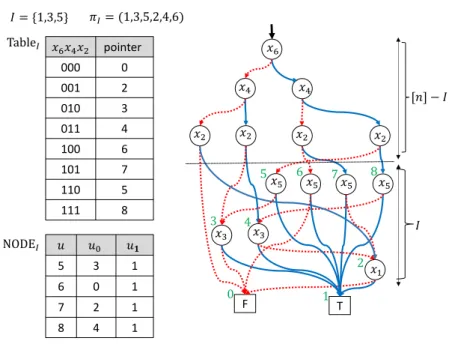
[𝑛] − 𝐼 𝑥' 𝑥( 𝑥( 𝑥) 𝑥) 𝑥) 𝑥) 𝑥* 𝑥* 𝑥* 𝑥* 𝑥+ 𝑥+ 𝑥, T F 𝐼 0 1 3 4 2 5 6 7 8 𝑢 𝑢7 𝑢𝟏 5 3 1 6 0 1 7 2 1 8 4 1 NODE= 𝑥'𝑥(𝑥) pointer 000 0 001 2 010 3 011 4 100 6 101 7 110 5 111 8 Table= 𝐼 = {1,3,5} 𝜋₌= (1,3,5,2,4,6)

Figure 4Examples of data structures used in AlgorithmFS: tableIandnodeIwithI={1,3,5} for the OBDD (rhs) representingf(x1, . . . , x6) =x1x2+x3x4+· · ·+x5x6 for the variable ordering (x1, x3, x5, x2, x4, x6). The pointers (integers) to the nodes labeled withx1, x3, x5 are each shown at

the top-left positions of the nodes.

∅ 𝑛

Each dot corresponds to ℱ𝒮(𝐼)for a subset 𝐼 ⊂ 𝑛 of size 𝑘 𝑘 𝑘 − 1

𝑖

= argmin

mincost

𝜋

= 𝜋

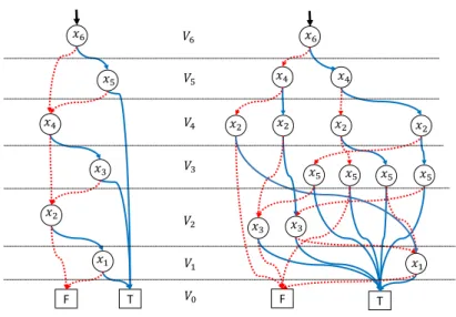
Figure 5Schematic view of Friedman-Supowit Algorithm. The algorithm goes from the left to the right. On the vertical line indicated by k, there are n_kdots, each of which corresponds to F S(I) for a subsetI⊆[n] of sizek. F S(I) is computed fromF S(hI\ii) for alli∈I, which are arranged as dots on the line indicated byk−1 and have already been computed.

36:18 Quantum Algorithm for Finding the Optimal Variable Ordering for BDDs

given the partial OBDD for

𝜋

!

and

𝐽 ⊆ 𝑛 ∖ 𝐾

,

produces the partial OBDD for

𝜋

!⊔#

in time

𝑂

∗

2

%& ! & #

3

#

time/space.

𝐼

ℱ𝒮(𝐼 ⊔ 𝐽) ℱ𝒮(𝐼)

|𝐼 ⊔ 𝐽|

Figure 6Schematic view ofFS∗. This view corresponds to the case wherem= 1 andJ⊂[n]\I

in Lemma 8. The shaded area is the one thatFS∗sweeps to produceF S(hI, Ji).

ℱ𝒮( 𝐼, 𝑛 ∖ 𝐼 )

This corresponds to

ℱ𝒮 𝐼

for

𝐼 ⊂ 𝑛

.

Output

𝜋

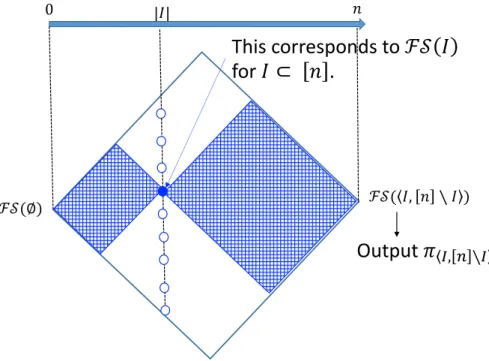
Figure 7Schematic view of Eq. (4) in Lemma 10. Intuitively, the lemma says that it is possible to decomposeFS∗into the parts each of which consists of the two shaded rectangles that share the dot corresponding toF S(I) on the line indicated by|I|for a subsetI⊆[n] of some fixed size. The optimal variable ordering is induced by one of the parts.

ℱ𝒮(∅)

ℱ𝒮( 𝑛 )

𝑘

Quantumly

find the

minimum

FS*

Computed in the

classical preprocess

(a truncation of FS*)

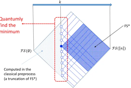
Figure 8Schematic view of our algorithm in the simplest case (one-parameter case). The dotted area is computed in the classical preprocess, which is realized by truncating the process ofFS∗as stated in Lemma 8. The shaded area is computed by usingFS∗. The actual algorithm runs the quantum minimum finding, which callsFS∗to coherently compute the shaded area corresponding to every dot on the vertical line indicated byk.