Probabilistic Calibration of Computer Model and Application to Reliability Analysis of Elasto-Plastic Insertion Problem

10th World Congress on Structural and Multidisciplinary Optimization

May 19 -24, 2013, Orlando, Florida, USA

Probabilistic Calibration of Computer Model and Application to Reliability Analysis of

Elasto-Plastic Insertion Problem

Min Young Yoo1, Joo Ho Choi2

1

Department of Aerosapce and Mechanical Engineering, Korea Aerospace University, Goyang-city, Republic of Korea, [email protected]

2

Center for Mechanical and Aerospace Reliability Engineering, Korea Aerospace University, Goyang-city, Republic of Korea, [email protected]

Computer model is a useful tool that gives solution by physical modeling instead of expensive testing. In the reality, however, it often disagrees due to the simplifying assumption and unknown or uncertain input parameters. In this study, a Bayesian approach is proposed, that calibrates the computer model in probabilistic way using the measured data. Elasto-plastic analysis of a pyrotechnically actuated device (PAD) is employed to demonstrate the approach, which is a component that delivers high power in remote environments by combustion of a self-contained energy source. A simple mathematical model that quickly evaluates the performance is developed. Unknown input parameters are calibrated conditional on the experimental data using Markov Chain Monte Carlo algorithm, which is a modern computational statistics method. Finally the results are applied to determine the reliability of the PAD.

Keywords: Pyrotechnically Actuated Device, Elasto-Plastic Analysis, Calibration, Markov Chain Monte Carlo 1. Inrtoduction

In various fields of engineering, experiments are often conducted for the design of a device and its validation, which is in most cases time-consuming or even impossible due to many limitations. Thus, efforts have been exerted to develop a simple but well-fitted model that simulates the underlying physics. The simulation has been actively applied to various fields and is regarded now as necessary process in the industries. However, the simulation performance is generally limited by simplifying assumptions, unknown input parameters and computing performance, which often leads to the disagreement from the reality in more or less degree. In order to resolve this issue, there have been various studies on calibration of the difference between the simulation and experiment. The most common and simple practice has been to tune some unknown parameters of the model to match the experiments via trial and error, which was usually implemented in the deterministic way. During the process, however, several uncertainties exist in the model including the model error and insufficient information of input parameters, and in the experiment including the limited number of tests and measurement error. Recently, there have been active research on how to account for these uncertainties in the model calibration. For instance, Bayarri et al. [1] studied on probabilistic calibration of input parameters based on the field data for the spot weld and automotive crash problems. Bayesian approach is employed to calibrate unknown parameters, which can estimate the parameters in the form of probability distribution conditional on the field data. Then the simulation results are given by the predictive interval, instead of a single value.

The objective of this study is to apply the same method to the calibration of the model of pyrotechnic actuated device (PAD). PAD is a device that delivers high power in remote environments by combustion of a self-contained energy source. The PAD function consists of two steps with one being the explosive combustion within the chamber, and the other the piston insertion due to the generated pressure from the chamber into the housing to activate the intended operation. As the device is to perform critical functions in the aerospace and defense applications, the performance analysis as well as its reliability assessment is needed at the design phase. The analysis is however demanding because of its nonlinearity and some unknown parameters. In this study, a simple mathematical model for the piston insertion that involves elasto-plastic deformation is developed. Unknown parameters are calibrated based on the field data, which are obtained in the form of probability distribution, reflecting the associated uncertainties. Then, the results are used as the input to evaluate the reliability of the PAD function. In section 2, brief explanations are given to the PAD, and elasto-plastic insertion model of the piston. In section 3, Bayesian formulation is addressed for the model calibration, followed by the sampling algorithm Markov Chain Monte Carlo(MCMC) that brings us the distributions of the calibrated parameters. Before calibration, approximation model is introduced to implement MCMC more efficiently instead of the original model. Section 4 conducts the reliability analysis using the crude Monte Carlo simulation based on the posterior distributions of the parameters obtained in section 3. The distinguishing feature of the current approach is that instead of employing the arbitrary assumed distributions for unknown input parameters, calibrated distributions

(a) before activation (b) after activation Figure 1: Illustration of PAD

are used for the reliability analysis, which are more trustworthy. 2. Pyrotechnically Actuated Device

2.1. Pyrotechnically Actuated Device

Pyrotechnically actuated device (PAD) takes a variety of forms such as pin pullers, cable cutters, pyro-valves and so on. In this study, the target device is a valve type as shown in Figure 1, which is introduced by [2]. The figure is just a conceptual introduction of the operating principles. Actual shape is more complex than as it appears, but is not given here due to the proprietary reason. The mechanism of this device is as follows. Once the combustion and expansion of gas arise in the chamber shown in the upper part, high gas pressure exerts the piston to move into the small space toward bottom. The cutter installed on tip of the piston penetrates the diaphragm that encloses nitrogen gas. As the gas flows out of this device, the operation is activated. In this regard, the PAD plays the role of valve that opens a gas flow. According to the mechanism, in the PAD analysis, analytical model can be integrated by two disciplines that are coupled with each other. First is the analysis of explosive combustion within an actuator and resulting gas flow in an expansion chamber. Second is the elasto-plastic analysis that simulates insertion of tapered piston into the housing by the pressure generated in the chamber. While the former is relatively well established over the times, the latter is less paid attention. So the main objective of the study is to develop a mathematical model that can evaluate the piston movement against the housing under the given pressure history. A straightforward solution for this is to employ commercial FEA code, which is, however, computationally demanding in case of reliability analysis. In this study, simpler model is proposed to obtain solution in much faster way based on the closed form analysis under some assumptions.

2.2. Elasto-Plastic Insertion Model

Tapered piston in Figure 1(a) undergoes large deformation as it is forced into the housing as shown in Figure 1(b). As a result, contact pressure is generated around the contact surface between the piston and the housing. Then the friction force is generated that resists the movement of the piston due to the pressure. The resistance force can be expressed as a function of the position of the piston. In order to calculate this, the main idea is that during the piston insertion, each cross sectional segment of the piston and outer housing is assumed as a shrink fit of two cylindrical

(a) segments (b) cross-section of segment

members with given interference, as is shown in Figure 2. Figure 2(a) and (b) show cross sectional segments along the movement direction and the top view of each segment, respectively. Depending on the degree of interference, the inner and outer part may undergo elastic, elasto-plastic or full plastic deformation. Tresca criterion is employed to identify plastic part, in which linear strain hardening rule is used for plasticity, which consists of the yield strength and strain hardening parameter that represents the tangent modulus. The interface pressure is computed by closed form solution for each of these cases. The resistance force is obtained by applying friction coefficient to these and integrating the axial components over the whole interface. The analytical model is constructed in this way and more detail about the process is given in reference [2] and [3]. MATLAB is used for the implementation, in which the resistance force is computed at 51 displacement points along the range of 2.5mm with the interval being 0.05mm. Though not addressed here, commercial code ANSYS is also employed to solve the problem, which takes 10 minutes or more. On the other hand, the MATLAB model takes only 1~2 seconds for the same problem, which reduces the computing time remarkably while producing the similar solutions.

2.3. Unknown Parameters

The resistance force calculated by the elasto-plastic insertion analysis of PAD is affected by several input parameters, which include the material properties such as Young’s modulus, Poisson’s ratio, plastic behavior and shapes of the piston and housing. Among these, there are some unknown parameters that are not easy to characterize by separate lab test or too costly to measure. They are the strain hardening parameter of the piston and the coefficient of friction at the interface. Consequently, these parameters are estimated and calibrated in this study based on the experimental data.

3. Calibration and Validation

3.1. Bayesian approach for model calibration

In this study, Bayesian theory is employed to address the calibration in the following form



|





|

  

f



y



f y



f



(1)

where



is the unknown parameter to estimate, which consist of the coefficient of friction and the strain hardening parameter,

y

is the experimental data, is likelihood of the data under the given , is the prior distribution of and is the posterior distribution that are updated by the data . The theory states that our degree of belief on the unknown parameters is given by a probability distribution that is updated by the measured data from the prior knowledge. Assuming that the error between the model and the measurement of the resistance force follow a normal distribution with zero mean and standard deviation



, the posterior distribution of the unknown parameter can be expressed by



₂

  

₂ / 2 1



 



2

1

, |

exp

'

2

n e e M e M

y

y

y

y

y

 





 





















(2)

where is measured resistance force, is resistance force by the model and

n

is the number of the data. In this study, the prior distribution is not applied due to the ignorance of the prior knowledge. Based on this expression, one can obtain the posterior distribution of the unknown parameters. For the practical implementation, sampling method such as MCMC are used as is addressed in the following section.

3.2. Markov Chain Monte Carlo

Markov Chain Monte Carlo (MCMC) is a sampling algorithm that stochastically estimates uncertainties of unknown parameters and determines the distribution of each parameter based on measured data. In this method, initial value was set and Markov Chain sampling in which the previous value affects the next value is used. As a result, influence of the initial value disappears eventually and only samples that reflect uncertainties based on field data are accumulated. Generally, for this, calculations of 104 times are required. From that, it is possible to obtain probability distribution and the output is given by the confidence bounds, which have adequately accounted for the uncertainties conditional on the given experimental data. There are various ways to implement the Markov Chain algorithm such as Gibbs sampling. In this study, the Metropolis-Hastings algorithm, which is an algorithm commonly used in the MCMC, is adopted.

3.3. Approximation Model

3.3.1. Necessity of Approximation Model



|



f y





f

 





f





|y



y

e

The MATLAB model, taking about 1.7 seconds on average to calculate the resistance force with respect to the displacement, is very efficient program compared to the ANSYS. In spite of it, about 5 hours is consumed to run a single MCMC for sampling of 104 numbers. Besides several runs are needed as the trial and error to find out proper setups for the successful runs of the algorithm. Therefore, in order to further reduce the computation time, an approximation model that substitutes the analytical model needs to be developed.

3.3.2. Approximation Model

MATLAB analytical model for the resistance force is given as as follows, where is the piston displacement, and is the set of unknown parameters, which include the coefficient of friction and strain hardening parameter .

 

,



, ,



M M M

y



y

z





y

z

 

₍₃₎

Now we would like to establish an approximation model using the regression technique that can replace the original model and computes the response in much quicker way. For the approximation, we put symbol ^ as follows.





ˆ

_M

ˆ

_M

, ,

y



y

z

 

(4)

In order to establish the approximation model with respect to the displacement, 3rd-degree and 5th-degree polynomials are attempted by regression at 11 points with arbitrary



and



at 0.2 and 0.35 respectively. The fitted results are compared with the original response as shown in Figure 3, from which we can find the 5th degree model fits the original very precisely. So the 5th degree model is chosen as follows

5 1 2 3 4 5 0 1 2 3 4 5 0 ˆ n M n n y b z b b z b z b z b z b z  



      (5) 0 0.5 1 1.5 2 2.5 -200 -100 0 100 200 300 400 500 600 700 Displacement (mm) R e s is tanc e F o rc e ( N ) Regression Analysis computer model 3rd 5th mu=0.2 eta=0.35 0 0.5 1 1.5 2 2.5 0 1000 2000 3000 4000 5000 6000 7000 8000 Displacement (mm) R e s is tanc e F o rc e ( N ) Computer Model mu=0.2 eta=0.35 mu=0.1 eta=0.35 mu=0.2 eta=0.5

Figure 3: Regression analysis of computer model Figure 4: Effect of coefficient of friction and strain hardening parameter on resistance force

0.2 0.4 0 200 400 600 b0 mu b0 0.2 0.4 -6000 -4000 -2000 0 2000 b1 mu b1 0.2 0.4 0 2 4 6 8x 10 4_b2 mu b2 0.2 0.4 -6 -4 -2 0x 10 4_b3 mu b3 0.2 0.4 0 5000 10000 15000 b4 mu b4 0.2 0.4 -200 -100 0 100 200 b5 mu b5 0.2 0.4 0 200 400 600 b0 eta b0 0.2 0.4 -6000 -4000 -2000 0 2000 b1 eta b1 0.2 0.4 0 2 4 6 8x 10 4_b2 eta b2 0.2 0.4 -6 -4 -2 0x 10 4_b3 eta b3 0.2 0.4 0 5000 10000 15000 b4 eta b4 0.2 0.4 -200 -100 0 100 200 b5 eta b5

Figure 5: Effect of coefficient of friction on

b

n Figure 6: Effect of strain hardening parameter on

b

n M

y

z





where ~ are the polynomial coefficients to be fitted via the original responses. By the way, these coefficients are again functions of two unknown parameters because they change with respect to the two parameters as shown in Figure 4. In order to investigate these behaviors, polynomial regression is carried out and the coefficients are determined at each grid point of the two parameters ranging from 0.1 to 0.5. The resulting figures are given in Figure 5 and Figure 6 which exhibit the functions in terms of a parameter while fixing the other parameter at a constant. Based on this observation, we can approximate all the coefficients by 2nd order polynomial with respect to the two parameters as follows

2 2

0 1 2 3 4 5

n n n n n n n

b







     







   



(6)

where means

m

th coefficient of . Therefore, to build an approximation model, total of 36 of are obtained and the approximation model is constructed as follows.









5 0

ˆ

_M

, ,

_n

,

n n

y

z

 

b

 

z







_{0.1  0.5, 0.1  0.5} (7) 3.4. Calibration

In this section, by using the approximation model (7), calibration is performed using the MCMC algorithm. Before applying the real experimental data, virtual data are generated and used for the calibration as a preliminary step in Section 3.4.1. Then in the next section, real calibration of parameters is performed using the field data. 3.4.1. Calibration Based on Virtual Data

Using the MATLAB model, 26 virtual data were generated which play the role of experimental data. The values used are , and measurement error are assumed to follow normal distribution, with

400

  . Assuming that we don’t know the true values for , and



, MCMC using the polynomial approximation model is performed based on the data. As a result, posterior distributions of two parameters and



can be obtained as shown in Figure 7. The mean values of these are



0.2114,



0.3330 and



425.6.

0 0.05 0.1 0.15 0.2 0.25 0.3 0.35 0 5000 10000 15000 Coefficient of Friction 0 0.05 0.1 0.15 0.2 0.25 0.3 0.35 0.4 0.45 0.5 0 2000 4000 6000 8000

Strain Hardening Parameter

Figure 7: Posterior distribution of two parameters using the virtual data

0 0.5 1 1.5 2 2.5 -1000 0 1000 2000 3000 4000 5000 6000 7000 8000 Displacement (mm) R e s is tanc e F o rc e (N ) MCMC (virtual data) virtual data true model y_m y_l y_u

Figure 8: Posterior predictive distribution using the virtual data





~ 0, N 

0.35





0.2











nm



bn



nm bn 0

b

b

₅

It can be confirmed that they are close to the true values. Using the distributions of the two parameters, we can simulate the resistance force and get the posterior predictive distribution with respect to the displacement, which are shown in Figure 8. As expected, the mean of the predictive distribution denoted by is close to the true model. The 95% predictive bounds given by and enclose the data quite well. Consequently, it is concluded that the proposed method calibrates the unknown parameters correctly conditional on the data and the predicted results include the uncertainty quite well.

3.4.2. Calibration Based on Field Data

In this section, by using the 99 field data which are obtained through the real experiment, MCMC is performed similar to the section 3.4.1. As a result, posterior distributions of the two parameters are as shown in Figure 9, and their mean values and measurement error are obtained as



0.280,



0.1051 and



571.8. From this, predictive distribution is obtained in Figure.10. Unlike the previous example in 3.3.1, the model and data show significant difference. This may be attributed to the simplifying assumption for the MATLAB model which is the segmentation of the device and application of interference fit of concentric cylinders. In the future, we should study on how to overcome this difference. Nevertheless, favorable results are obtained from the field data because the prediction bounds encloses all the field data, which indicates that the model is as reliable as it is based on the assumptions and field data, and can be used in the future simulation.

4. Reliability Analysis 4.1. Definition of Failure

The posterior distributions of unknown parameters acquired in the previous section are used for reliability analysis of the PAD. In order to do this, we need to define failure. As shown in Figure 1, the PAD is regarded as failure if it stops before reaching the target distance that cuts the diaphragm. This occurs when the pressure is not enough from the chamber or when the resistance force is too large. According to Newton’s 2nd law, the piston motion can be expressed by the equation:

 

2 2 p R

d

m

z

F

F

dt





(8) 0.2 0.25 0.3 0.35 0 0.5 1 1.5 2x 10 4 Coefficient of Friction The Posterior Distribution (field data)

4 0.090 0.1 0.11 0.12 0.13 0.14 0.15 0.16 0.5 1 1.5 2x 10 4

Strain Hardening Parameter

Figure 9: Posterior distribution of two parameters with field data

0 0.5 1 1.5 2 2.5 -2000 -1000 0 1000 2000 3000 4000 5000 6000 7000 8000 Displacement (mm) R e s is tanc e F o rc e (N ) MCMC (field data) field data y_m y_l y_u

Figure 10: Posterior predictive distribution using the field data

u

y

m

y

l

where

m

, and are piston mass, pressure force and resistive force, respectively. can be obtained by combustion analysis coupled with the piston motion. In this study, however, it is assumed given a priori with respect to the time for the sake of convenience. The resistance force in this equation is the same as the model given in eq. (7). While input parameters are the two parameters and in the previous sections, more parameters exhibiting uncertainty are added here in the reliability analysis. Equation (8) is solved to obtain the displacement history of the piston over the time, from which the final distance of the piston is obtained as . Let us denote the critical distance that the piston should reach as . Then the limit state function can be expressed as follows.

 

p

 

f

g X



z

X



z

(9)

and failure probability is defined as



0



P g



. (10)

4.2. Analysis and Result 4.2.1 Input Parameter

In the computer model , input parameters consist of 9 parameters including and that were calibrated in section 3. The information are stated in Table 1. Only the distribution type and coefficient of variation (COV) of the parameters are given here for proprietary reason. Materials of the piston and housing are STS303 and STS630 respectively. Young’s modulus and yield strength are assumed by Weibull distributions. Dimensions of each cylinder are assumed by normal distributions.

4.2.2. Calculation

In order to determine failure probability, crude Monte Carlo simulations are carried out. In this case, the calculation is made by the MATLAB model, not the approximation model because it cannot consider the input parameters except the unknown parameters



and



. Also the command ‘parfor’ is used for parallel computation, in order to save computing time, which enables the division of calculation by the number of cores of the computer.

Table 1: Properties of input parameter

Input Parameter Distribution COV

Inner cylinder Young’s modulus Weibull 5%

Yield strength Weibull 5%

Radius Normal 2%

Outer cylinder Young’s modulus Weibull 5%

Yield strength Weibull 5%

Inner radius Normal 2%

Outer radius Normal 2%

Coefficient of friction - -

Strain hardening parameter - -

-0.50 0 0.5 1 1.5 2 2.5 3 0.5 1 1.5 2 2.5 3 g = z_p - z_f The Frequency Diagram

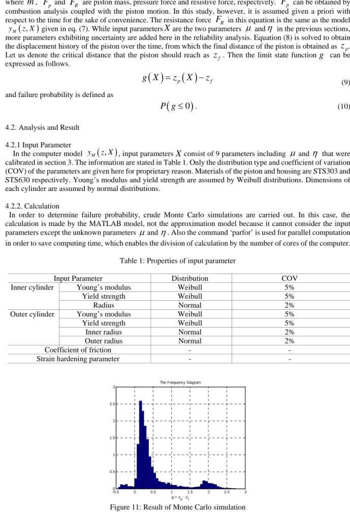
Figure 11: Result of Monte Carlo simulation



,



M y z X

X









p

z

f

z

g

p

F

F

_R

F

p R

F



,



M y z X

X

Random samples with 104 numbers are generated for the input parameters according to the Table 1, in which the two calibrated parameters are taken from the samples already made by the MCMC. Limit state function

g

are calculated using the generated samples. As a result, the failure probability is obtained as . Also the frequency diagram of the

g

values is given in Figure 11, in which the area less than 0 is the failure probability 0.0359.

5. Conclusion

In this study, a simplified analytical model is established for the elasto-plastic piston insertion model in the PAD. The unknown parameters in this model are calibrated in the probabilistic way using the Bayesian formulation, which estimates the parameters as the posterior distribution conditional on the field data. MCMC is employed as the numerical implementation tool to obtain the unknown parameters in the form of samples. In the model, the coefficient of friction and the strain hardening parameter are given as the unknown parameters, which are not easy to measure in the lab experiments. In order to further facilitate the computation, polynomial approximation model is developed in addition and used in the MCMC implementation that determines the posterior distribution of the two parameters. The method proves to be useful as is found in the virtual data example. The model is then applied to the calibration based the real experimental data in the same way. Unlike the case of the virtual data, however, the prediction does not closely match the field data. Nevertheless, the predictive bounds favorably enclose the field data, which proves that the model is as reliable as it is based on the model and the field data. Reliability analysis is carried out using the 9 input variables to obtain the failure probability of the PAD function. Probability distributions of the two variables are taken from the posterior distributions of the previous run while the others are assumed by existing distributions as specified in Table 1. Crude Monte Carlo simulation with the total of 104 numbers is conducted, from which the failure probability of PAD is obtained.

In this study, several limitations are observed. First, as shown in Figure 10, substantial difference between the prediction by the analytical model and the field data is observed. This may be due to the modeling assumption to accommodate numerical efficiency. One option is to develop more elaborate model to reduce the gap between the two, but the efficiency will be compromised instead. Otherwise, the bias can be dealt with from the Bayesian view point, which can be used to compensate the difference. The detail can be found in the reference [1]. Second is about the range of the two unknown parameters, both of which are arbitrarily bounded between 0.1 and 0.5 in the approximation model. As a result, the posterior distribution of the strain hardening parameter seems to be limited at the lower bound as shown in Figure 9, which implies that the value may be lower than 0.1. This problem can be avoided by using the MATLAB model directly, instead of the approximation model in the MCMC implementation, which leads to the much longer computing time.

5.References

[1] M.J. Bayarri, J.O. Berger, D. Higdon, M.C. Kennedy, A. Kottas, R. Paulo, J. Sacks, J.A. Cafeo, J. Cavendish, C.H. Lin and J. Tu, A Framework for Validation of Computer Models, National Institute of Statistical Sciences, 2002.

[2] Adam M. Braud, Keith A. Gonthier and Michele E. Decroix, System Modeling of Explosively Actuated Valves , Journal of Propulsion and Power, Vol.23, No.5, 1080-1095, 2007.

[3] Ahmet N. ERASLAN and Tolga AKIS, Deformation Analysis of Elastic-Plastic Two Layer Tubes Subject to Pressure: an Analytical Approach, Turkish Journal of Engineering and Environmental Sciences 28, 261-268, 2004.

[4] M.C. Kennedy and A. O’Hagan, Bayesian Calibration of Computer Models, Journal of the Royal Statistical Society, Series B, 63, 423-462, 2001



0



0.0359