Jan de Leeuw and Patrick Mair
Simple and Canonical Correspondence Analysis Using the R Package
anacor
Article (Published) (Refereed)
Original Citation:
de Leeuw, Jan and Mair, Patrick (2009) Simple and Canonical Correspondence Analysis Using the R Package anacor. Journal of Statistical Software, 31 (5). pp. 1-18. ISSN 1548-7660
This version is available at: http://epub.wu.ac.at/5020/ Available in ePubWU: April 2016
ePubWU, the institutional repository of the WU Vienna University of Economics and Business, is provided by the University Library and the IT-Services. The aim is to enable open access to the scholarly output of the WU.
This document is the publisher-created published version. It is a verbatim copy of the publisher version.
August 2009, Volume 31, Issue 5. http://www.jstatsoft.org/
Simple and Canonical Correspondence Analysis
Using the
R
Package
anacor
Jan de Leeuw
University of California, Los Angeles
Patrick Mair
WU Wirtschaftsuniversit¨at Wien
Abstract
This paper presents theRpackageanacorfor the computation of simple and canonical correspondence analysis with missing values. The canonical correspondence analysis is specified in a rather general way by imposing covariates on the rows and/or the columns of the two-dimensional frequency table. The package allows for scaling methods such as standard, Benz´ecri, centroid, and Goodman scaling. In addition, along with well-known two- and three-dimensional joint plots including confidence ellipsoids, it offers alternative plotting possibilities in terms of transformation plots, Benz´ecri plots, and regression plots. Keywords:anacor, correspondence analysis, canonical correspondence analysis,R.
1. Introduction
Correspondence analysis (CA;Benz´ecri 1973) is a multivariate descriptive method based on a data matrix with non-negative elements and related to principal component analysis (PCA). Basically, CA can be computed for any kind of data but typically it is applied to frequencies formed by categorical data. Being an exploratory tool for data analysis, CA emphasizes two-and three-dimensional graphical representations of the results.
In this paper we briefly review the mathematical foundations of simple CA and canonical CA in terms of the singular value decomposition (SVD). The main focus is on the computational implementation inR(RDevelopment Core Team 2009), on scaling methods based on Benz´ecri distances, centroid principles, and Fischer-Maung decomposition and on the elaboration of corresponding graphical representations. More details about CA, various extensions and related methods can be found in Greenacre (1984), Gifi (1990) and Greenacre and Blasius
(2006) and numerous practical issues are discussed inGreenacre(2007).
Recently, several relatedRpackages have been implemented and updated, respectively. Theca
on standardized residuals. Multiple CA is carried out in terms of SVD on either the indicator matrix or the Burt matrix. Joint CA, which can be regarded as a variant of multiple CA excluding the diagonal cross tabulations when establishing the Burt matrix, can be performed as well as subset CA. The package provides two- and three-dimensional plots of standard and principal coordinates with various scaling options.
The ade4 package (Chessel, Dufour, and Thioulouse 2004; Dray, Dufour, and Chessel 2007;
Dray and Dufour 2007) which has been developed in an ecological context, allows for multiple CA, canonical CA, discriminant CA, fuzzy CA and other extensions. Another related package is vegan (Dixon 2003; Oksanen, Kindt, Legendre, O’Hara, Henry, and Stevens 2009), also developed in the field of ecology, which allows for constrained and partially constrained CA as well. Another related package ishomals (de Leeuw and Mair 2009) which fits models of the Gifi-family (homogeneity analysis aka multiple CA, nonlinear PCA, nonlinear canonical correlation analysis). Additional CA-related packages and functions in R can be found in
Mair and Hatzinger(2007).
Theanacorpackage we present offers, compared to the packages above, additional possibilities for scaling the scores in simple CA and canonical CA, additional graphical features including confidence ellipsoids. It also allows for missing values which are imputed using Nora’s algo-rithm (Nora 1975). The package is available from the ComprehensiveRArchive Network at
http://CRAN.R-project.org/package=anacor.
2. Simple correspondence analysis
2.1. Basic principles of simple CAThe input unit of analysis is a bivariate frequency table F having n rows (i= 1, . . . , n) and
mcolumns (j = 1, . . . , m). Thus thefij are non-negative integers. Without loss of generality
we suppose thatn ≥m. The row marginals fi• are collected in a n×n diagonal matrix D
and the column marginalsf•j in am×mdiagonal matrixE. Supposeun andum are vectors
of lengthsnandmwith all elements equal to 1. It follows that the grand total can be written asn=u0nF um.
Suppose we want to find row scores and column scores such that the correlation in the bivariate tableF is as large as possible. This means maximizingλ(x, y) =n−1x0F yover the row score vectorxand column score vector y. These vectors arecentered by means of
u0nDx= 0, (1a)
u0mEy= 0, (1b)
andnormalized on the grand mean by
x0Dx=n, (1c)
y0Ey=n. (1d)
Such vectors, i.e., both centered and normalized, are calledstandardized.
In order to solve the constrained optimization ofλ(x, y) over the vectors (x, y) satisfying the conditions above we form the Lagrangian using undetermined multipliers (ξx, ξy, µx, µy) and
set the derivatives equal to zero. Thus, the optimal x and y must satisfy the centering and normalization conditions in (1), as well as the stationary equations
F y=ξxDx+µxDu, (2a)
F0x=ξyEy+µyEu. (2b)
By using the side constraints (1) we find that the Lagrange multipliers must satisfyξx =ξy =
σ(x, y) and µx=µy = 0. Thus we can solve the simpler system
F y=σDx, (3a)
F0x=σEy, (3b)
together with the side conditions in (1). The system in (3) is a singular value problem. We find the stationary values ofσ as the singular values of
Z =D−12F E− 1
2. (4)
Sincem≤n, we have the singular value decompositionZ =PΣQ0. P isn×nand composed of the left singular vectors; Q is m×m and composed of the right singular vectors. Both matrices are orthonormal, i.e., P0P = Q0Q = I. Σ is the diagonal matrix containing the min(n, m) =m singular values in descending order.
Them solutions of the stationary equations (3) can be collected in
X =√nD−12P, (5a)
Y =√nE−12Q, (5b)
whereX is then×m of row scores andY ism×m. Except for the case of multiple singular values, the solutions are uniquely determined. If (x, y, σ) solves (3) we shall call it asingular triple, while the two vectors (x, y) are a singular pair. In total there are s = 0, . . . , m−1 singular triples (xs, ys, σs) wherexs and ys are the columns of X and Y respectively.
We still have to verify if themcolumns ofX and Y satisfy the standardization conditions in (1). First, X0DX = nP0P =nI and Y0EY = nQ0Q= nI, which means both X and Y are normalized. In fact we haveorthonormality, i.e., if (xs, ys, σs) and (xs0, ys0, σs0) are different
singular triples, thenx0sDxs0 = 0 andys0Eys0 = 0.
To investigate centering, we observe that (un, um,1) is a singular triple, which is often called
the trivial solution, because it does not depend on the data. All other singular triples (xs, ys, λs) with σs<1 are consequently orthogonal to the trivial one, i.e., satisfyu0nDx= 0
and u0mEy = 0. If there are other singular triples (xs, ys,1) with perfect correlation, then
xs and ys can always be chosen to be orthogonal to un and um as well. It follows that all
singular triples define stationary values ofσ, except for (un, um,1) which does not satisfy the
centering conditions.
The squared singular valuesσ2 correspond to the eigenvaluesλofZ0Z and ZZ0, respectively. Let us denote the corresponding diagonal matrix of eigenvalues by Λ. In classical CA termi-nology (see e.g. Greenacre 1984) these eigenvalues are referred to as principal inertias. By ignoringλ0based on the trivial triple (x0, y0,1), the Pearson decomposition can be established
by means of n m−1 X s=1 σs2=n m−1 X s=1 λs=n(tr Z0Z−1) =χ2(F). (6)
χ2(F) is called total inertia and corresponds to the Pearson chi-square statistic for indepen-dence of the table F with df = (n−1)(m−1). The single composites are the contributions of each dimension to the total inertia. Correspondingly, for each dimension a percentage reflecting the contribution of dimension sto the total intertia can be computed. The larger the eigenvalue, the larger the contribution. In practical applications, a “good” CA solution is characterized by large eigenvalues for the first few dimensions.
2.2. Methods of scaling in simple CA
The basic plot in CA is the joint plot which draws parts of X and Y jointly in a low-dimensional Euclidean space. Note that instead of joint plot sometimes the term CA map is used. Both symmetric and asymmetric CA maps can be drawn with theca package and corresponding descriptions are given inNenadic and Greenacre(2007).
We provide additional methods for scaling X and Y which lead to different interpretations of the distances in the joint plot. Ideally we want the dominant geometric features of the plot (distances, angles, projections) to correspond with aspects of the data. So let us look at various ways of plotting row-points and column-points in p dimensions using the truncated solutionsXp which isn×p, and Yp which ism×p.
In the simplest case we can use the standardized solution ofXp andYp without any additional
rescaling and plot the coordinates into a device. This corresponds to a symmetric CA map and the coordinates are referred to asstandard coordinates.
An additional option of scaling is based on Benz´ecri distances, also known as chi-square distances. A Benz´ecri distance between two rows iandk is defined by
δik2(F) = m X j=1 fij fi• − fkj fk• 2 /f•j. (7)
If we use ei and ek for unit vectors of lengthn, then
δik2(F) = (ei−ek)0D−1F E−1F0D−1(ei−ek) = = (ei−ek)0D− 1 2ZZ0D− 1 2(ei−ek) = = (ei−ek)0D− 1 2PΣ2P0D− 1 2(ei−ek) = = (ei−ek)0XΣ2X0(ei−ek).
Thus, the Benz´ecri distances between the rows of F are equal to the Euclidean distances between the rows of XΣ. Again, Xp is the row scores submatrix and Σp the submatrix
containing the first p ≤ m −1 singular values. Based on these matrices fitted Benz´ecri distances can be computed. It follows that
dik(X1Σ1)≤dik(X2Σ2)≤ · · · ≤dik(Xm−1Σm−1) =δik(F). (8)
In the same way the Euclidean distances between the rows of YΣ approximate the Benz´ecri distances between the columns ofF. In CA terminology this type of coordinates is sometimes referred to as principal coordinates of rows and columns. Based on these distances we can compute a Benz´ecri root mean squared error (RSME) for the rows and columns separately (see alsode Leeuw and Meulman 1986). For the rows it can be expressed as
RM SE = s 1 n(n−1) X i X k (δik(F)−δik(XpΣp))2. (9)
A third way to scale the scores is based on thecentroid principle. The row centroids (averages) expressed by means of the column scores areX(Y) =D−1F Y. In the same way, the column centroids are given by Y(X) = E−1F0X. These equations will be used in Section 5.1 to produce the regression plot. Using this notation, the stationary equations can be rewritten as
X(Y) =XΣ, (10a)
Y(X) =YΣ. (10b)
This shows that for each singular triple (x, y, σ) the regression ofy on x and the regression of x on y are both linear, go through the origin, and have slopesλ and λ−1. Depending on whetherX and/or Y are centered, the distances between the points in the joint plot can be interpreted as follows. Suppose that we plot the standard scores ofXp together with Y(Xp).
Distances between column points approximate Benz´ecri distances and distances between row points and column points can be interpreted in terms of the centroid principle. Observe that in this scaling the column points will be inside the convex hull of the row points, and if the singular values are small, column points will form a much smaller cloud than row-points. The same applies if we reverse the role ofXp andYp. If we plotY(Xp) andX(Yp) in the plane,
then distances between row points in the plane approximate Benz´ecri distances between rows and distances between column points in the plane approximate Benz´ecri distances between columns. Unfortunately, distances between row points and column points do not correspond directly to simple properties of the data.
A further possibility of scaling isGoodman scaling which starts with the Fisher-Maung de-composition. Straightforwardly, Z =PΣQ0 can be rewritten as nD−12F E−
1 2 =D 1 2XΣY0E 1 2. It follows that nF = DXΣY0E. Now we plot the row-points XpΣ
1 2
p and the column points
YpΣ
1 2
p. The scalar product of the two sets of points approximatesXΣY0, which is the matrix
of Pearson residuals (trivial dimension removed)
nfij
fi•f•j
−1. (11)
For this Goodman scaling there does not seem to be an obvious interpretation in terms of distances. This is somewhat unfortunate because people find distances much easier to understand and work with than scalar products.
It goes without saying that if the singular values in Σp are close to one, the four different joint
plots will be similar. Generally, plots based on the symmetric Benz´ecri and Goodman scalings will tend to be similar, but the asymmetric centroid scalings can lead to quite different plots.
3. Canonical correspondence analysis
3.1. Basic principles of canonical CATer Braak (1986) presented canonical CA within an ecological context having the situation where the whole dataset consists of two sets: data on the occurrence or abundance of a number of species, and data on a number of environmental variables measured which may
help to explain the interpretation of the scaled solution. In other words, they are incorporated as effects in the CA computation in order to examine their influence on the scores.
To give a few examples outside ecology, in behavioral sciences such environmental variables could be various types schools, in medical sciences different hospitals etc. Thus, from this particular point of view canonical CA reflects multilevel situations in some sense; from a general point of view it reflects any type of effects on the rows and/or columns of the table. We introduce canonical CA from the general perspective of having covariatesA on the row margins fi• and/or covariates B on the column margins f•j. Hence, canonical CA can be
derived by means of a linear regression ofAandBon the row scoresX and the column scores
Y, i.e.
X=AU, (12a)
Y =BV, (12b)
whereA and B are known matrices of dimensionsn×aand m×b, respectively, and U and
V are weights. We suppose, without loss of generality, thatA andB are of full column rank. We also suppose that un is in the column-space of A and um is in the column-space of B.
Note that ordinary CA is a special case of canonical CA in which bothAand B are equal to the identity.
By using basically the same derivation as in the previous section, we find the singular value problem
(A0F B)V = (A0DA)UΣ, (13a)
(B0F0A)U = (B0EB)VΣ. (13b)
Analogous to Section2.1, X and Y, expressed by means of (12), satisfy the standardization conditionsU0A0DAU =nI andV0B0EBV =nI. Ifun=Agandum=Bh, then (g, h) defines
a solution to (13) with σ = 1. Thus we still have the dominant trivial solution which makes sure that all other singular pairs are centered.
The problem that we have to solve is the SVD onZ which for canonical CA can be expressed as
Z = (A0DA)−12A0F B(B0EB)− 1
2 (14)
using the inverse of the symmetric square roots of A0DA and B0EB. Suppose again that
Z = PΣQ0 is the singular value decomposition of Z. Then U = (A0DA)−12P and V = (B0EB)−12Qare the optimal solutions for the weights in our maximum correlation problem, and the corresponding scores are
X=A(A0DA)−12P, (15a)
Y =B(B0EB)−12Q. (15b)
BothX and Y are normalized, orthogonal, and, except for the dominant solution, centered. Again,XandY are the standard coordinates which can be rescaled by means of the principles described in Section 3.2.
If we assume, for convenience, that un is the first column of A and um is the first column
which is equal to one. The other (a−1)(b−1) elements of Z are, under the hypothesis of independence, asymptotically independentN(0,1) distributed. Thus
n p X s=1 σ2s =n p X s=1 λs=n(trZ0Z−1) =χ2(FA,B), (16)
which is asymptotically a chi-square with df = (a−1)(b−1). Hence, in canonical CA we compute a canonical partition of the components of chi-square corresponding with orthogonal contrastsA and B.
3.2. Methods of scaling in canonical CA
In this section the same methods of rescaling of row and column scores used for simple CA, are applied to canonical CA. Again, we start with Benz´ecri distances δik2 (FAB) between two
rowsiand k and using unit vectorsei and ek of length n:
δ2ik(FAB) = (ei−ek)0(A0DA)−1A0F B(B0EB)−1B0F0A(A0DA)−1(ei−ek) = = (ei−ek)0(A0DA)− 1 2ZZ0(A0DA)− 1 2(ei−ek) = = (ei−ek)0(A0DA)− 1 2PΣ2P0(A0DA)− 1 2(ei−ek) = = (ei−ek)0XΣ2X0(ei−ek) = = (ei−ek)0AUΣ2U0A0(ei−ek).
Analogous to (8) the monotonicity property holds for the distances for the first p singular values in terms of the row scores submatrix Xp and the singular value submatrix Σp. The
Benz´ecri distances for the columns can be derived in an analogous manner.
For the centroid principle we rewrite the stationary equations in (13) as follows (cf. Equa-tion 10):
A(A0DA)−1A0DX? =XΣ, (17a)
B(B0EB)−1B0EY? =YΣ, (17b)
where the site scores are given by
X?=D−1F Y =X(Y), (17c)
Y? =E−1F0X=Y(X), (17d)
and of courseX =AU andY =BV. We see that the columns of X are proportional to the projections in the metricDofX?on the space spanned by the columns ofA. The same applies to the column scoresY. Note that if we solve the linear regression problem of minimizing
tr (X?−AT)0D(X?−AT) (18) then the minimizer is T = (A0DA)−1A0DX?. As a solution of the stationary equations is follows thatT =UΣ. Ter Braak(1986) callsT thecanonical coefficients. In our more general setup there are also canonical coefficients for the columns, which are the regression coefficients when regressingY? onB.
Within the context of canonical CA there are various matrices of correlation coefficients that can be computed to give canonical loadings. For the rows, we can correlate X, X?, and A
(intraset correlations). If the columns of A are centered and normalized, the correlations become Σ. For the columns, the situation is the same forY, Y? and B. The package returns the site scores, the intraset correlations, and the canonical loadings.
The Fisher-Maung decomposition is merely a rewriting of the singular value decomposition. The most obvious generalization in the constrained case uses
(A0DA)−12A0F B(B0EB)− 1 2 =PΣQ0, (19a) or (A0DA)−1A0F B(B0EB)−1 =UΣV0, (19b) or A0F B= (A0DA)UΣV0(B0EB) =A0(DXΣY0E)B. (19c) This can be written asA0RB= 0 with
rij =fij −fi•f•j(1 + c−1 X s=1 σsxisyjs), (20) wherec=min(a, b).
Note that the joint plots pertaining to the different scaling methods are again based on the
p-dimensional solution with the corresponding row scoresXp based on the linear combination
of matrix A, and the corresponding column scores Yp based on the linear combination of
matrixB.
4. Additional topics
4.1. Confidence ellipsoids using the delta methodThe core computation in theanacor package is the SVD on Z = PΣQ0. As a result we get then×mmatrixP of left singular vectors, them×mmatrixQof the right singular vectors, the diagonal matrix Σ of order m containing the singular values, and, correspondingly, the eigenvalue matrix Λ. Based on these results the n×p row score matrix Xp and the m×p
column score matrix are computed (standard scores). At this point an important issue is the replication stability of the results in terms of confidence ellipsoids around the standard scores in the joint plot.
A general formal framework to examine stability in multivariate methods is given in Gifi
(1990, Chapter 12). The starting point of the replication stability is the well-known delta method. Let us assume that we have a sequence of asymptotically normal random vectorsxn.
Thus √n(xn−µ)
D
→ N(0,Σ). If we apply a transformation φ(xn) the delta method states
that√n(φ(xn)−φ(µ))≈ √
n∇φ(µ)(xn−µ)
D
→N(0,∇φ(µ)0Σ∇φ(µ)). In simple words: The delta method provides the transformed variance-covariance (VC) matrix which is based on the gradient ofφ evaluated atµ.
To apply this method for CA we have to embed our observationspij =fij/ninto a sequence
of random variables, i.e., a sequence of multinomial distributed random variables with cell probabilitiesπij. Asymptotic theory states that
√
n(p−π)→D N(0,Π−ππ0) wherep andπ are the vectors of relative frequencies and probabilities and Π is the diagonal matrix with the elements ofπ on the diagonal.
The transformation of the proportions to the singular values and vectors are given by the equations in (3). Expressions for the partial derivatives ∂p∂φ
ij are long and complicated, and
not very informative. They are special cases of the partials for the generalized singular value decompositions given in (de Leeuw 2007, Section 2.2.1). For CA they were given earlier by
O’Neill(1978a,b) and Kuriki(2005).
4.2. Reconstitution algorithm for incomplete tables
As an additional feature of theanacorpackage, incomplete tables are allowed. The algorithm we use was proposed by Nora(1975) and revised by de Leeuw and van der Heiden(1988). This algorithm should not be mistaken for the CA reconstitution formula which allows for the reconstruction of the data matrix from the scores. Nora’s algorithm is rather based on the complementary use of CA and log-linear models (seevan der Heiden and de Leeuw 1985) and provides a decomposition of the residuals from independence. It is related, however, to Greenacre’s joint correspondence analysis (JCA) for multivariate data (Greenacre 1988). We will describe briefly the reconstitution of order 0 which is implemented inanacor.
We start at iteration l = 0 by setting the missing values in F to zero. The corresponding table which will be iteratively updated is denoted by F(0). Correspondingly, the row margins
are fi(0)• , the column margins f•(0)j and the grand meanf••(0). The elements of the new table F(1) are computed under independence. Pertaining to iterationl, this corresponds to
fij(l+1) = f (l) i• f (l) •j f••(l) . (21)
Within each iteration a measure for the change in the frequencies is computed, i.e., H(l) =
Pn i=1 Pm j=1f (0) ij logf (l)
ij . The iteration stops if|H(l)−H(l−1)|< . After reaching convergence,
we set F := F(l) and we proceed with the computations from Section 2 and Section 3, respectively.
5. Applications of simple and canonical CA
5.1. Plotting options in anacor
The basic function in the package is anacor which performs simple or canonical CA with different scaling options. The NA cells in the table will be imputed using the reconstitution algorithm. The results are stored in an object of class "anacor". For objects of this class a
print and a summarymethod is provided. Two-dimensional plots can be produced with the
plot method, static scatterplot3d plots (Ligges and M¨achler 2003) with the plot3dstatic
method and dynamicrglplots (Adler and Murdoch 2009) with theplot3dmethod. The type of the plot can be specified by the argument plot.type:
"jointplot": Plots row and column scores into the same device (also available as 3-D).
"rowplot","colplot": Plots the row/column scores into separate devices (also avail-able as 3-D).
"graphplot": This plot type is an unlabeled version of the joint plot where the points are connected by lines. Options are provided (i.e., wlines) to steer the line thickness indicating the connection strength.
"regplot": Regression plots are conditional plots on the weighted score averages. First, the unscaled solution is plotted. Conditional on a particular category of one variable, the expected value (i.e., the weighted average score) of the other variable is plotted. This is done for both variables which leads to two regression lines within one plot. Second, the scaled solition is taken and plotted in the same manner.
"transplot": The transformation plot plots the initial row/column categories against
the scaled row/column scores.
"benzplot": The Benz´ecri plot shows the observed distances against the fitted Benz´ecri distances; assumed that the row and/or columns in the CA result are Benz´ecri scaled. For the rows the observed distances are based on D−12ZZ0D−
1
2 and the fitted distances on XpΣ2pXp0; for the columns on E−
1
2ZZ0E− 1
2 and YpY0
p, respectively.
"orddiag": The ordination diagram for CCA produces a joint plot and includes the
column and row covariates based on intraset correlations.
In addition,anacoroffers various CA utility functions: expandFrame()expands a data frame into a indicator supermatrix, burtTable() establishes the Burt matrix, and mkIndiList()
returns a list of codings with options for crisp indicators, numerical versions, and fuzzy coding. 5.2. Applications of simple CA
We start with an application of simple CA on Tocher’s eye color data (Maung 1941) collected on 5387 Scottish school children. This frequency table consists of the eye color in the rows (blue, light, medium, dark) and the hair color in the columns (fair, red, medium, dark, black).
R> library("anacor") R> data("tocher")
R> res <- anacor(tocher, scaling = c("standard", "centroid")) R> res
CA fit:
Sum of eigenvalues: 0.2293315
Total chi-square value: 1240.039 Chi-Square decomposition:
Chisq Proportion Cumulative Proportion
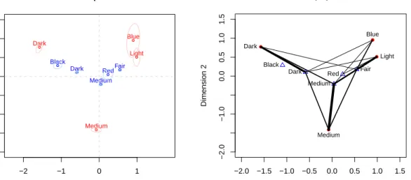
● ● ● ● −2 −1 0 1 −2.0 −1.0 0.0 0.5 1.0 1.5 Joint plot Dimension 1 Dimension 2 ● ● ● ● ● Blue Light Medium Dark Fair Red Medium Dark Black ● ● ● ● ● ● ● ● ● ● ● ● ● −2.0 −1.5 −1.0 −0.5 0.0 0.5 1.0 1.5 −2.0 −1.0 0.0 0.5 1.0 1.5 Graphplot Dimension 1 Dimension 2 Blue Light Medium Dark Fair Red Medium Dark Black
Figure 1: Joint plot and graph plot for Tocher data.
Component 2 162.077 0.131 0.996
Component 3 4.630 0.004 1.000
R> plot(res, plot.type = "jointplot", xlim = c(-2, 1.5), ylim = c(-2, 1.5), + asp = 1)
R> plot(res, plot.type = "graphplot", xlim = c(-2, 1.5), ylim = c(-2, 1.5), + wlines = 5, asp = 1)
For this two-dimensional solution we use asymmetric scaling by having standard coordinates for the rows and principal coordinates for the columns. As graphical representation methods the joint plot including 95% confidence ellipsoids and the graph plot are chosen (see Figure1). As mentioned above the coordinates of the points in both plots are the same. Note that the column scores (blue points) in the joint plot are scaled around their centroid. The row scores (red points) are not rescaled. In the graph plot the columns scores are represented by blue triangles and the row scores by red points. The thickness of the connecting lines reflect the frequency of the table or, in other words, the strength of the connection. The distances within row/column categories can be interpreted and we see that black/dark hair as well as fair/red hair are quite close to each other. The same applies to blue/light eyes. The distances between single row and column categories can not be interpreted.
We can run a χ2-test of independence
R> chisq.test(tocher)
Pearson's Chi-squared test
data: tocher
and see that it is highly significant. Looking at theχ2-decomposition of the CA result we see that the first component accounts for 88.6% of the totalχ2-value (i.e., inertia).
In a second example we show two CA solutions for the Bitterling dataset (Wiepkema 1961) which concerns the reproductive behavior of male bitterlings. The data are derived from 13 sequences using a moving time-window of size two (time 1 in rows, time 2 in columns) and are organized in a 14×14 table with the following categories: jerking (jk), turning beats (tu), head butting (hb), chasing (chs), fleeing (ft), quivering (qu), leading (le), head down posture (hdp), skimming (sk), snapping (sn), chafing (chf), and finflickering (ffl).
We fit a two-dimensional and a five-dimensional CA solution using Benz´ecri scaling. With two dimensions we explain 53.2% of the total inerita (sum of eigenvalues is 1.33) and with five dimensions we explain 85.8% (sum of eigenvalues is 2.15).
R> data("bitterling")
R> res1 <- anacor(bitterling, ndim = 2, scaling = c("Benzecri", "Benzecri")) R> res2 <- anacor(bitterling, ndim = 5, scaling = c("Benzecri", "Benzecri")) R> res2
CA fit:
Sum of eigenvalues: 2.147791
Benzecri RMSE rows: 0.0002484621
Benzecri RMSE columns: 0.000225833
Total chi-square value: 14589.07 Chi-Square decomposition:
Chisq Proportion Cumulative Proportion
Component 1 4026.287 0.276 0.276 Component 2 3730.218 0.256 0.532 Component 3 1996.814 0.137 0.669 Component 4 1635.673 0.112 0.781 Component 5 1145.514 0.079 0.859 Component 6 904.313 0.062 0.921 Component 7 832.702 0.057 0.978 Component 8 284.566 0.020 0.998 Component 9 31.421 0.002 1.000 Component 10 1.357 0.000 1.000 Component 11 0.206 0.000 1.000
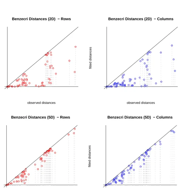
R> plot(res1, plot.type = "benzplot", main = "Benzecri Distances (2D)") R> plot(res2, plot.type = "benzplot", main = "Benzecri Distances (5D)")
The improvement of the five-dimensional solution with respect to the two-dimensional one is reflected by the Benz´ecri plots in Figure2. For a perfect (saturated) solution the points would lie on the diagonal. This plot can be used as an overall goodness-of-fit plot or, alternatively, single distances can be interpreted.
The data for the next example were collected byGlass (1954). In this 7×7 table the occupa-tional status of fathers (rows) and sons (columns) of 3497 British families were cross-classified.
●● ● ● ● ● ● ● ● ● ● ● ● ●● ● ● ● ● ● ● ● ● ● ● ● ●● ● ● ● ● ● ● ● ● ● ● ● ● ● ● ● ● ● ● ● ● ● ●● ● ● ● ● ● ● ● ● ● ● ● ● ● ● ●● ●● ● ● ● ● ● ● ● ● ● ● ● ● ● ● ● ● ● ●● ● ● ● ● ● ● ● ● ● ● ●● ● ● ● ● ● ● ● ● ● ●● ● ● ● ● ● ● ● ● ●●●●● ● ● ● ● ● ● ● ● ●● ● ● ● ● ● ● ● ● ● ●
Benzecri Distances (2D) − Rows
observed distances fitted distances ● ● ● ● ● ● ● ● ● ● ● ● ● ● ● ● ● ● ● ●●● ● ● ● ● ●● ● ● ● ● ● ● ● ● ● ● ● ● ● ● ● ● ● ● ● ● ● ● ●● ● ● ● ● ● ● ● ● ● ● ● ● ● ● ● ● ● ● ● ● ● ● ● ● ● ● ● ● ● ● ● ● ● ● ● ● ● ● ● ● ●● ● ● ● ● ● ● ● ● ● ● ● ● ● ● ● ● ● ● ● ● ● ● ● ● ● ● ●●●● ● ● ● ● ● ● ● ● ●●● ● ● ● ● ● ● ● ● ●
Benzecri Distances (2D) − Columns
observed distances fitted distances ●● ● ● ● ● ● ● ●● ● ● ● ●● ● ● ● ● ● ● ● ● ● ● ● ●● ● ● ● ● ● ● ● ● ● ● ● ● ● ● ● ● ● ● ● ● ● ●● ● ● ● ● ● ● ● ● ● ● ● ● ● ● ● ● ● ● ● ● ● ● ●● ● ● ● ● ● ● ● ● ● ● ● ●● ● ● ● ● ● ● ● ● ● ● ●● ● ● ● ● ● ● ● ● ● ●● ● ● ● ● ● ● ● ● ● ● ● ●● ● ● ● ● ● ● ● ● ● ● ● ● ● ● ● ● ● ● ● ●
Benzecri Distances (5D) − Rows
observed distances fitted distances ● ● ● ● ● ● ● ● ● ● ● ● ● ● ● ● ● ● ● ● ● ● ● ●● ● ●● ● ● ● ● ● ● ● ● ● ● ● ● ● ● ● ● ● ● ● ● ● ● ●● ● ● ● ● ● ● ● ● ● ● ● ● ● ● ● ● ● ● ● ● ● ● ●● ● ● ● ● ● ● ● ● ● ● ● ● ● ● ● ● ● ● ● ● ● ● ● ● ● ● ● ● ● ● ● ● ● ● ● ● ● ● ● ● ● ● ● ● ● ● ● ● ● ● ● ● ● ● ● ● ● ● ●● ● ● ● ● ● ● ● ●
Benzecri Distances (5D) − Columns
observed distances
fitted distances
Figure 2: Benz´ecri plots for Bitterling data.
The categories are professional and high administrative (PROF), managerial and executive (EXEC), higher supervisory (HSUP), lower supervisory (LSUP), skilled manual and routine non-manual (SKIL), semi-skilled manual (SEMI), and unskilled manual (UNSK).
R> data("glass")
R> res <- anacor(glass)
R> plot(res, plot.type = "regplot", xlab = "fathers occupation", + ylab = "sons occupation", asp = 1)
Unscaled Solution Dimension 1
fathers occupation categories
sons occupation categor
ies
PROF HSUP SKIL UNSK
PR OF HSUP SKIL UNSK ● ● ● ● ● ● ● ● ● ● ● ● ● ● 50 19 26 8 18 6 2 16 40 34 18 31 8 3 12 35 65 66 123 23 21 11 20 58 110 223 64 32 14 36 114 185 714 258 189 0 6 19 40 179 143 71 0 3 14 32 141 91 106 −0.5 0.0 0.5 1.0 1.5 2.0 2.5 −0.5 0.0 0.5 1.0 1.5 2.0
Scaled Solution Dimension 1
fathers occupation scores
sons occupation scores
● ● ● ● ● ● ● ● ● ● ● ● ● ● 50 19 26 8 18 6 2 16 40 34 18 31 8 3 12 35 65 66 123 23 21 11 20 58 110 223 64 32 14 36 114 185 714 258 189 0 6 19 40 179 14371 0 3 14 32 141 91 106
UNSK LSUP EXEC PROF
UNSK LSUP HSUP EXEC PR OF
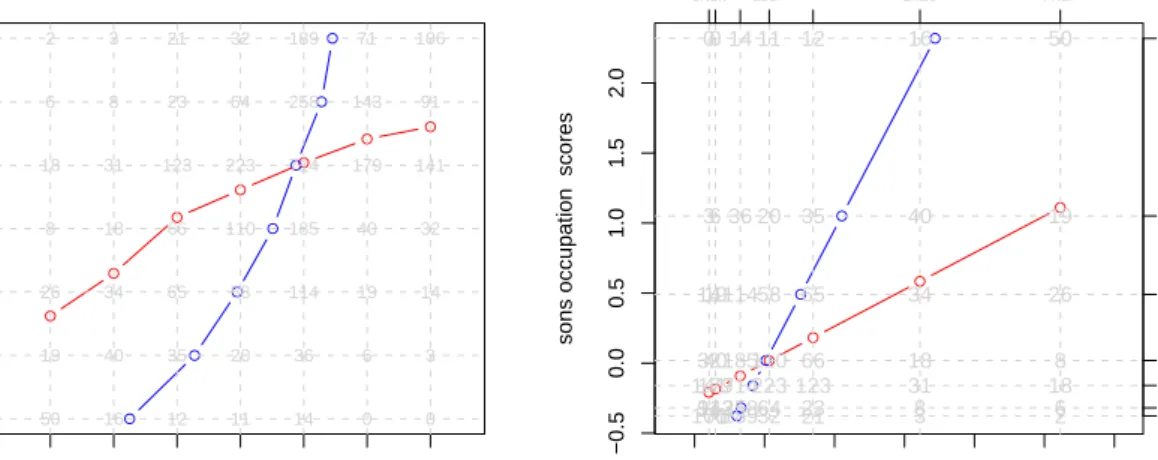
Figure 3: Regression plots for Glass data.
On the left hand side we show the unscaled solution. The father’s occupation is on the abscissae and the occupation of the sons on the ordinate. The grid represents the table with the corresponding frequencies. The red line is drawn conditional on the categories of father’s occupation: For each of these categories the expected value of son’s occupation is computed. Remind that before the CA computation the category values range from 1 to 7 (or m in general). The observed frequencies represent the weights for the category scores. Based on the scores and the weights we can compute the expected value of son’s occupation conditional on each category of father’s occupation. Analogously, the blue line represents the expected father’s occupation conditional on the son’s occupation. The monotonicity of both line is not surprising since the categories (professions) are ordered in the table (from PROF down to UNSK) and the variables are highly dependent (χ2= 1361.742,df = 36,p <0.000).
On the right hand side of Figure3we find the scaled solution. The first obvious characteristic is that the grid components are not equidistant anymore due to the category scaling performed by CA. The regression lines are computed in an analogous fashion than in the unscaled solution; with the exception that we operate on the transformed category scores. This leads to two linear “regressions” with the row/column scores as predictors. It is an important property of simple CA that the scores are always linearized. This phenomenon is known as bilinearizability. A thorough discussion is given in Mair and de Leeuw(2009).
5.3. Canonical CA on Maxwell Data
A hypothetical dataset byMaxwell(1961) is used to demonstrate his method of discriminant analysis. We will use it to illustrate canonical CA. The data consist of three criterion groups (columns), i.e., schizophrenic, manic-depressive and anxiety state; and four binary predictor variables each indicating either presence or absence of a certain symptom. The four symptoms are anxiety suspicion, schizophrenic type of thought disorders, and delusions of guilt. These
● ● ● ● ● ● ● ● ● ● ● ● ● ● ● ● −2 −1 0 1 −2.0 −1.0 0.0 0.5 1.0 1.5 Ordination Diagram Dimension 1 Dimension 2 ● ● ● 1 2 3 4 5 6 7 8 9 10 11 12 13 14 15 16 schizophrenic manic.depressive anxiety.disorder anxiety suspicion thought.disorders delusions.of.guilt ● ● ● ● ● ● ● ● ● ● ● ● ● ● ● ● −2.0 −1.0 0.0 0.5 1.0 1.5
Transformation Plot − Rows
row categories ro w scores ● ● ● ● ● ● ● ● ● ● ● ● ● ● ● ● 1 2 3 4 5 6 7 8 9 11 13 15 Dimension 1 Dimension 2
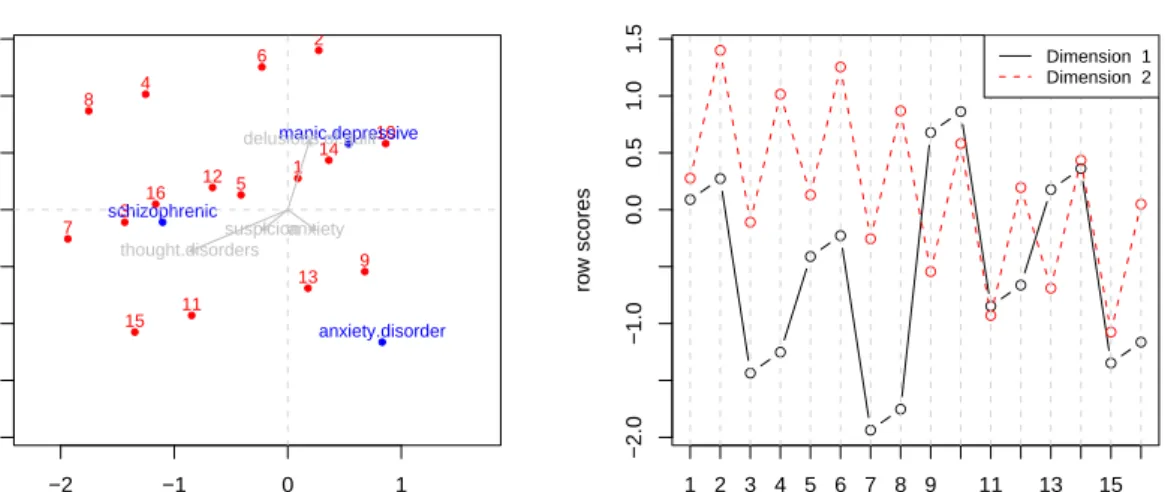
Figure 4: Ordination diagram and transformation plot for Maxwell data.
four binary variables were factorially combined to form 16 distinct patterns of symptoms (predictor patterns), and each of these patterns is identified with a row of the table. In total we have a cross-classification of 620 patients according to the 16 patterns of symptoms and the three criterion groups.
We fit a symmetric (Goodman scaled) two-dimensional solution and get an amount of ex-plained inertia of 87.2%.
R> data("maxwell")
R> res <- anacor(maxwell$table, row.covariates = maxwell$row.covariates, + scaling = c("Goodman", "Goodman"))
R> res
CA fit:
Sum of eigenvalues: 0.6553413
Total chi-square value: 406.312 Chi-Square decomposition:
Chisq Proportion Cumulative Proportion
Component 1 302.568 0.650 0.650
Component 2 103.743 0.223 0.872
R> plot(res, plot.type = "orddiag", asp = 1)
R> plot(res, plot.type = "transplot", legpos = "topright")
The ordination on the left hand side of Figure4is a joint plot including the covariates based on the intraset correlations. It shows that the mental diseases go into somewhat different
directions and thus they are not really related to each other. Furthermore we can see how each symptom pattern (determined by the covariates which are plotted as well) is related to each mental disease.
The transformation plot on the right hand side shows interesting patterns. For the first dimension a cyclic behavior over the predictors is identifiable. The scores (y-axis) for pairs of points 1-2, 3-4, 5-6, etc. do not change much within these pairs. Note that these pairs are contrasted by the (fourth) predictor “delusions of guilt”. Between these pairs some obvious differences in the scores are noticeable. These between-pairs-differences are contrasted by the (third) predictor “thought disorders”: 1-2 has 0, 3-4 has 1, 5-6 has 0 etc. Therefore, the first dimension mainly reflects thought disorders.
The second dimension shows an alternating behavior. Referring to the pair notation above, it reflects within-pair-differences based on “delusions of guilt”. In addition a slight downward trend due to “anxiety” (first predictor) can be observed.
6. Discussion
Theanacor package provides additional features which are not offered by other CA packages on CRAN. These features are additional scaling methods for simple and canonical CA, missing data, and graphical representations such as regression plots, Benz´ecri plots, transformation plots, and graphplots. The included utilities make it possible to switch from the data format used in anacor to the data format used in homals, and this gives the user a great deal of flexibility. The confidence ellipsoids from CA are a powerful tool to visualize the dispersions of the row and column projections in the plane.
References
Adler D, Murdoch D (2009). rgl: 3D Visualization Device System (OpenGL). R package version 0.84, URLhttp://CRAN.R-project.org/package=rgl.
Benz´ecri JP (1973). Analyse des Donn´ees. Dunod, Paris.
Chessel D, Dufour AB, Thioulouse J (2004). “The ade4 Package I: One-Table Methods.” RNews,4(1), 5–10. URLhttp://CRAN.R-project.org/doc/Rnews/.
de Leeuw J (2007). “Derivatives of Generalized Eigen Systems, with Applications.”Technical Report 528, UCLA Statistics Preprint Series. URL http://preprints.stat.ucla.edu/ download.php?paper=528.
de Leeuw J, Mair P (2009). “Gifi Methods for Optimal Scaling inR: The Package homals.” Journal of Statistical Software,31(4), 1–20. URL http://www.jstatsoft.org/v31/i04/. de Leeuw J, Meulman J (1986). “Principal Component Analysis and Restricted Multidimen-sional Scaling.” In W Gaul, M Schrader (eds.), Classification as a Tool of Research, pp. 83–96. North Holland Publishing Company, Amsterdam.
de Leeuw J, van der Heiden P (1988). “Correspondence Analysis of Incomplete Contingency Tables.”Psychometrika,53, 223–233.
Dixon P (2003). “vegan: A Package of R Functions for Community Ecology.” Journal of Vegetation Science,14, 927–930.
Dray S, Dufour AB (2007). “The ade4 Package: Implementing the Duality Diagram for Ecologists.” Journal of Statistical Software, 22(4), 1–20. URL http://www.jstatsoft. org/v22/i04/.
Dray S, Dufour AB, Chessel D (2007). “Theade4Package II: Two-Table and K-Table Meth-ods.”RNews,7(2), 47–52. URLhttp://CRAN.R-project.org/doc/Rnews/.
Gifi A (1990). Nonlinear Multivariate Analysis. John Wiley & Sons, Chichester. Glass DV (1954). Social Mobility in Britain. Free Press, Glencoe.
Greenacre MJ (1984).Theory and Applications of Correspondence Analysis. Academic Press, London.
Greenacre MJ (1988). “Clustering the Rows and Columns of a Contingency Table.” Journal of Classification,5, 39–51.
Greenacre MJ (2007). Correspondence Analysis in Practice. 2nd edition. Chapman & Hall/CRC, Boca Raton.
Greenacre MJ, Blasius J (2006). Multiple Correspondence Analysis and Related Methods. Chapman & Hall/CRC, Boca Raton.
Kuriki S (2005). “Asymptotic Distribution of Inequality-Restricted Canonical Correlation With Application to Tests for Independence in Ordered Contingency Tables.” Journal of Multivariate Analysis,94, 420–449.
Ligges U, M¨achler M (2003). “scatterplot3d – An R Package for Visualizing Multivariate Data.” Journal of Statistical Software, 8(11), 1–20. URL http://www.jstatsoft.org/ v08/i11/.
Mair P, de Leeuw J (2009). “A General Framework for Multivariate Analysis with Optimal Scaling: The R Package aspect.” Technical Report 561, UCLA Statistics Preprint Series. URLhttp://preprints.stat.ucla.edu/download.php?paper=561.
Mair P, Hatzinger R (2007). “Psychometrics Task View.” R News,7(3), 38–40. URL http: //CRAN.R-project.org/doc/Rnews/.
Maung K (1941). “Discriminant Analysis of Tocher’s Eye Color Data for Scottish School Children.” Annals of Eugenics,11, 64–67.
Maxwell AE (1961). “Canonical Variate Analysis When the Variables are Dichotomous.” Educational and Psychological Measurement,21, 259–271.
Nenadic O, Greenacre MJ (2007). “Correspondence Analysis in R, with Two- and Three-Dimensional Graphics: ThecaPackage.”Journal of Statistical Software,20(3), 1–13. URL
Nora C (1975).Une m´ethode de reconstitution et d’analyse de donn´ees incompl`etes [A Method for Reconstruction and for the Analysis of Incomplete Data]. Master’s thesis, Unpublished Th`ese d’Etat, Universit´e P. et M. Curie, Paris VI.
Oksanen J, Kindt R, Legendre P, O’Hara B, Henry M, Stevens H (2009). vegan: Community Ecology Package. Rpackage version 1.15-3, URL http://CRAN.R-project.org/package= vegan.
O’Neill ME (1978a). “Asymptotic Distribution of the Canonical Correlations From Contin-gency Tables.”Australian Journal of Statistics,20, 75–82.
O’Neill ME (1978b). “Distributional Expansions for Canonical Correlations From Contingency Tables.”Journal of the Royal Statistical Society B,40, 303–312.
RDevelopment Core Team (2009).R: A Language and Environment for Statistical Computing.
RFoundation for Statistical Computing, Vienna, Austria. ISBN 3-900051-07-0, URLhttp: //www.R-project.org/.
Ter Braak CJF (1986). “Canonical Correspondence Analysis: A New Eigenvector Technique for Multivariate Direct Gradients.”Ecology,67, 1167–1179.
van der Heiden P, de Leeuw J (1985). “Correspondence Analysis Used Complementary to Loglinear Analysis.”Psychometrika,50, 429–447.
Wiepkema PR (1961). “An Ethological Analysis of the Reproductive Behavior of the Bitterling (rhodeus amarus bloch).”Archives Neerlandais Zoologique,14, 103–199.
Affiliation: Jan de Leeuw
Department of Statistics
University of California, Los Angeles E-mail: [email protected]
URL: http://www.stat.ucla.edu/~deleeuw/
Patrick Mair
Department of Statistics and Mathematics WU Wirtschaftsuniversit¨at Wien
E-mail: [email protected]
URL: http://statmath.wu.ac.at/~mair/
Journal of Statistical Software
http://www.jstatsoft.org/published by the American Statistical Association http://www.amstat.org/
Volume 31, Issue 5 Submitted: 2008-11-25