Three Dimensional Hydrodynamic Modelling of Lake Erie: Kelvin Wave Propagation and Potential Effects of Climate Change on Thermal Structure and Dissolved Oxygen

(1)

Three Dimensional Hydrodynamic

Modelling of Lake Erie: Kelvin Wave

Propagation and Potential Effects of

Climate Change on Thermal Structure

and Dissolved Oxygen

by

Wentao Liu

A thesis

presented to the University of Waterloo in fulfillment of the

thesis requirement for the degree of Doctor of Philosophy

in

Applied Mathematics

(2)

(3)

I hereby declare that I am the sole author of this thesis. This is a true copy of the thesis, including any required final revisions, as accepted by my examiners.

(4)

(5)

Abstract

This thesis investigates physical processes in Lake Erie, a large, shallow mid-latitude lake, from two perspectives: climate change impacts on the thermal structure and dissolved oxygen concentration and small-scale eddy dynamics generated by internal Kelvin wave propagation. A three-dimensional hydrodynamic and aquatic ecological coupled model ELCOM-CAEDYM, validated by the field data collected in 2008, is first used to investi-gate the responses of the thermal structure and dissolved oxygen concentration in Lake Erie to potential changes in air temperature and wind speed. A new method is pre-sented to define spatially and temporally varying regions for the epilimnion, thermocline, and hypolimnion. Four metrics are selected to quantify the characteristics of the ther-mal structure: mean epilimnion temperature, mean hypolimnion temperature, onset and breakdown of stratification, and thermocline depth. Exploiting the power of the three dimensional model to provide a more authentic characterization of thermal structure in such large lakes, it is shown that patterns inferred from simple isotherm dynamics, as typ-ically done with one dimensional models, are not always accurate. In the dissolved oxygen studies similar analyses are presented. Three factors related to lake hydrodynamics have strong influences on hypolimnetic hypoxia: water temperature, stratification duration, and hypolimnion thickness. In a warm and quiescent year the hypolimnetic hypoxia will likely become more severe if considering the effects of meteorological forcing changes only. The present results show the potential for complicated and interactive effects of climate forcing on important biogeochemical processes in Lake Erie as well as other large mid-latitude lakes. Taking advantage of high performance computing, the generation of eddies when a baroclinic Kelvin wave propagates past a peninsula is studied using the MITgcm. The grid resolution can be refined from 2 km to 200 m in the parallel computing environment. With the finer resolution small-scale processes which cannot be resolved in the coarse resolution applied previously are able to be explored. The eddy dynamics are studied in detail in both an idealized lake and in Lake Erie. This work presents a first attempt at simulating small-scale hydrodynamic processes in large lakes and contributes to our understanding of how energy is moved from large scales (the scale of the basins in Lake Erie) to smaller scales (the scale of the peninsula or Point Pelee).

(6)

(7)

Acknowledgements

First and foremost, I would like to thank my supervisor Dr. Kevin Lamb. Counting my Master’s it has been more than six years, and Kevin has greatly influenced my de-velopment as a researcher and as a person. I am extremely grateful for his inspiration, guidance, encouragement, financial support, and not to mention the extra efforts of editing my mediocre English writing. More than just a supervisor, Kevin has been a good friend as well as a strong competitor in soccer and cycling.

I would like to thank my committee members Dr. Jinyu Sheng, Dr. Ralph Smith, Dr. Marek Stastna, and Dr. Francis Poulin for taking the time to review my thesis and provide valuable guidance. I thank Marek for numerous helpful discussions on my projects and his leadership in short-table ping pong, basketball, soccer, field trip, beer, BBQ, and “success at success”. The CAEDYM setup and tuning were conducted by Dr. Serghei Bocaniov, Dr. Ralph Smith, Dr. Luis Leon, and their colleagues in the Department of Biology. Thanks also go to Dr. Leon Boegman and Dr. Ram Yerubandi for their guidance during collaboration. Ship time in the field was courtesy of Environment Canada (NWRI) and Ontario Ministry of Natural Resources (Wheatley). Part of this work was made possible by the high performance computing facilities SciNet and SHARCNET.

I would like to thank everyone in the fluids group for creating such an enjoyable work environment: Dr. Waite, Nancy, Kris, Michael, Chris, Tim, Anton, Derek, Jason, Sina, Subasha, Jared, Robbie, Aaron, Yangxin, Georges, and Vladimir. Thanks also go to my good friends from the department in the teaching team, soccer buddies, and immigration group: Rahul, Venkata, Andree, Ruibin, Alex, and Wilten. I would also like to express my appreciation to the department staff Stephanie and Helen and Robyn from MFCF. Thank 72 wonderful Management Engineering class of 2017 students that I had a delightful first ever teaching semester. I would like thank my high school math teacher Mr. Tianyun Liu for proving me a solid foundation in mathematics and his great inspiration.

Most importantly, I would like to thank my family. I thank my little cousin Dan at WLU for all the joys she brings in the past four years. I am grateful to my parents who always believe in me and encourage me. To let me acquire top-notch education is always their higher priority, even it means that we can only have several weeks of family time every year. There is no word to express my appreciation and gratefulness, and I love you both! Finally I would like to thank my fiancée and my love Yang. Time does fly when one is in love. From Harbin to Vancouver, to Waterloo, St. Catharines, and Calgary, it has been eleven years since we first met. I am so lucky to have you by my side. Without your support I could not have achieved my goals. You are my deepest love and I will always

(8)

(9)

Dedication

(10)

(11)

List of Tables

3.1 Deployment details at meteorological stations by NWRI in 2008 . . . 23

3.2 A list of variables used in converting wind speeds to 10 m height . . . 30

3.3 Deployment details at mooring stations by NWRI in 2008 . . . 37

4.1 Responses in the mean epilimnion temperature. . . 66

4.2 Responses in the mean hypolimnion temperature . . . 66

4.3 Responses of the stratification breakdown time based on the number of stratified grid-columns . . . 67

4.4 Responses of the stratification duration based on the 18◦_{C contours} _{. . . .} ₆₇

4.5 Impacts due to air temperature and wind speed changes . . . 75

4.6 Responses in the mean epilimnion DO . . . 85

4.7 Responses in the mean hypolimnion DO . . . 85

5.1 Flow past a circular cylinder using the MITgcm setup . . . 102

5.2 Idealized internal Kelvin wave simulations setup . . . 117

5.3 Group 1: effects of the horizontal eddy viscosity Ah . . . 118

5.4 Group 2: effects of the lateral boundary condition . . . 125

(16)

5.7 Group 5: effects of the peninsula width with fixed Lp = 5 km . . . 128

5.8 Group 6: effects of the upwelling length and position . . . 133

(17)

List of Figures

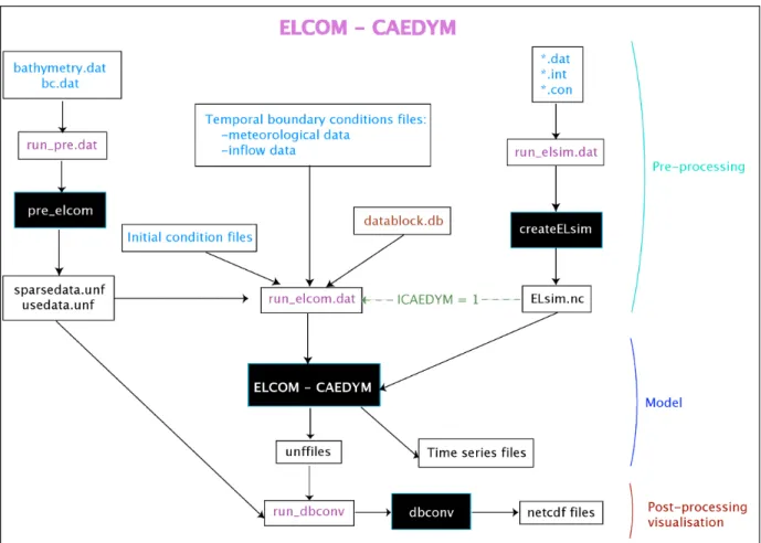
2.1 ELCOM-CAEDYM organization (from CAEDYM User Manual 2006).. . . 10

2.2 The MITgcm can be applied to a wide range of phenomenon, from convection on the left to the global circulation on the right (from MITgcm Manual 2013). 12

2.3 The global annual mean Earth’s energy budget from March 2000 to May 2004 (from Trenberth et al. 2009). . . 13

2.4 Typical thermal stratification of a temperate lake. . . 16

2.5 Two-dimensional representation of the effects of wind on a stratified lake: (a) to (c) stages in the development of the epilimnetic wedge and of shear instability at the downwind end of the thermocline; (d) isotherm distribution in Windermere, northern basin, after about 12 hours of relatively steady wind (from Mortimer 1974). . . 17

2.6 A long Kelvin wave in a uniform depth model (fromMortimer 1974). . . . 18

2.7 A standing Poincaré wave in a wide, rotating channel of uniform depth (from Mortimer 1974). . . 20

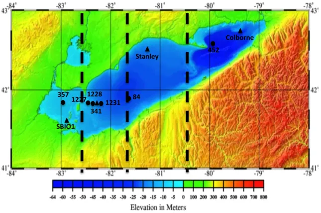
3.1 Available meteorological stations in Lake Erie from both NWRI (maple leaf) and NDBC (star). The elevation and bathymetry map is from the NOAA Great Lakes Environmental Research Laboratory (GLERL). . . 24

3.2 Solar radiation comparison in 2009 at: (A) EC452 and EC341, and (B) EC452 and NARR. . . 25

(18)

3.4 Relative humidity comparison in 2009 at: (A) EC452 and EC341, and (B) EC452 and NARR. . . 27

3.5 Air temperature comparison in 2008 at: (A,C) EC341 and NARR, and (B,D) EC Colborne and NARR. . . 28

3.6 (A) EC Colborne wind speeds comparison at 5 m and 10 m above, and (B) NDBC SBIO1 wind speeds comparison at 21 m and 10 m above. . . 31

3.7 Lake Erie bathymetry (from GLERL) with four forcing sections (divided by dash lines) and the locations of meteorological buoys (N) and thermistor

chains ( ). . . 34

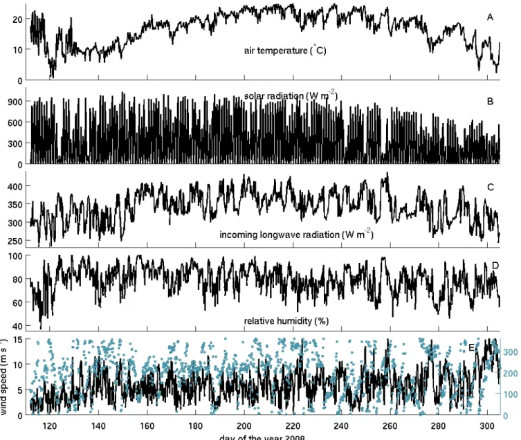
3.8 Time series of 3-hour averaged meteorological data at station 341: (A) air temperature, (B) solar radiation, (C) downward longwave radiation, (D) rel-ative humidity, and (E) wind speed (lines) and wind direction (dots, mea-sured clockwise from north in direction wind is coming from). . . 35

3.9 Contour plots: the observed (A-C) and EL-CD modelled (D-F) temperature comparison at (A,D) station 357, (B,E) 1227, and (C,F) 341. Line plots: (G) mean surface temperature; (J) station 357 at−1m; station 1227 at (H)

−1 m and (K) −8m; and station 341 at (I) −6m and (L) −15 m.. . . 40

3.10 Contour plots: the observed (A-C) and EL-CD modelled (D-F) temperature comparison at (A,D) station 1231, (B,E) 84, and (C,F) 452. Line plots: station 1231 at (G) −7 m and (J) −16m; station 84 at (H) −5 m and (K)

−20 m; and station 452 at (I)−20 m and (L) −40m. . . 41

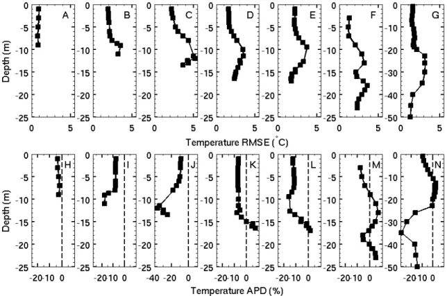
3.11 The vertical profiles of the root mean square error (RMSE, top panels) and the average percentage difference (APD, bottom panels) between the modelled and observed temperature at stations: (A,H) 357, (B,I) 1227, (C,J) 1228, (D,K) 1231, (E,L) 341, (F,M) 84, and (G,N) 452. . . 42

3.12 Contour plots: velocities (m s−1_{) comparison at station 341: (A) observed}

and (C) modelled east-west U, (B) observed and (D) modelled north-south V. Line plots: U (left panels) and V (right panels) at station 341 at: (E,F) −3 m; (G,H)−6 m; (I,J) −9 m; and (K,L)−12 m. . . 44

(19)

3.15 Upper half: observed (A-C) and EL-CD modelled (D-F) DO (mg L−1₎

pro-file comparison at station 1228 (A,D), 341 (B,E), and 1231 (C,F). Lower half: observed (G-I) and EL-CD modelled (J-L) temperature (◦_{C) profile}

comparison at station 1228 (G,J), 341 (H,K), and 1231 (I,L). . . 47

3.16 Top panels: station 1228 at (A) 5 mab, (D) 3 mab, (G)0.5mab; station 341

at (B) 3 mab, (E) 2 mab, (H) 1 mab, (K) 0.5 mab; station 1231 at (C) 5

mab, (F) 2 mab, (I) 1 mab, (L)0.5mab; (J) station 84 at 0.5mab. Bottom

panels: DO RMSE at stations: (M) 1231, (N) 341, and (O) 1231. . . 48

3.17 MODIS satellite image near Rondeau on Aug 28 (from NASA). . . 49

3.18 Meteorological stations used in 2012 simulations (bathymetry from GLERL). Three computational domains are divided by the dot lines. . . 50

3.19 Meteorological forcing at Port Stanley: (A) air temperature, (B) wind di-rection, and (C) wind speed. . . 51

3.20 Surface temperature at (A) 12:00, 17 Aug 2012 and (B) 06:00, 01 Sep 2012. 52

4.1 The modelled temperature profiles at station (A) 1231 and (B) 452. The black line is the calculated thermocline, two white lines are the epilimnion and hypolimnion boundaries withcepi =chyp = 25%, and the blue line is the

epilimnion boundary using the definition in Carignan et al. (2000).. . . 59

4.2 The modelled temperature profiles at station (A) 1231 and (B) 452. The lines are calculated epilimnion and hypolimnion boundaries with: cepi =

chyp = 15% (purple), 25% (white), and35% (blue). . . 60

4.3 Mean temperature response to the air temperature changes in: (A,F) west-ern basin, (B,G) central basin epilimnion, (C,H) eastwest-ern basin epilimnion, (D,I) central basin hypolimnion, and (E,J) eastern basin hypolimnion. The upper five are the mean temperature and the lower five are the difference from the base case. . . 68

4.4 Total number of stratified grid-columns in response to air temperature change in (A) central basin and (B) eastern basin, where the dash line is 25%of the

total number of water grid-columns and the dot line is 10%. The right label

shows the percentage of the total basin surface area. The 18◦_{C contours in}

(C) central basin and (D) eastern basin. Mean thermocline depth in (E) central basin and (F) eastern basin. Please refer to Fig. 4.3 for the colour

(20)

4.5 Mean thermocline depth in October when the air temperature is changed by: (A) −4◦C, (B) −2◦C, (C) −1◦C, (D) +1◦C, (E) +2◦C, (F) +4◦C, and

when the wind speed is changed by: (G) −20%, (H) −10%, (I) −5%, (J) +5%, (K) +10%, (L) +20%. . . 70

4.6 Mean temperature response to the wind speed changes in: (A,F) western basin, (B,G) central basin epilimnion, (C,H) eastern basin epilimnion, (D,I) central basin hypolimnion, and (E,J) eastern basin hypolimnion. The upper five are the mean temperature and the lower five are the difference from the base case. . . 73

4.7 Total number of stratified grid-columns in response to wind speed change in (A) central basin and (B) eastern basin, where the dash line is 25% of the

total number pf water grid-columns and the dot line is10%. The right label

shows the percentage of the total basin surface area. The 18◦_{C contours in}

(C) central basin and (D) eastern basin. Mean thermocline depth in (E) central basin and (F) eastern basin. Please refer to Fig. 4.6 for the colour legend. . . 74

4.8 Temperature (◦_{C) contours at station 1231 (western central basin) with the}

air temperature changed by: (A) −4◦C, (B) −2◦C, (C) −1◦C, (D) 0 (base

case), (E) +1◦C, (F) +2◦C, and (G) +4◦C. The blue lines are calculated

thermoclines. . . 79

4.9 Temperature (◦_{C) contours at station 452 (eastern basin) with the air}

tem-perature changed by: (A)−4◦C, (B)−2◦C, (C)−1◦C, (D) 0 (base case), (E) +1◦C, (F)+2◦C, and (G)+4◦C. The blue lines are calculated thermoclines. 80

4.10 Temperature (◦_{C) contours at station 1231 (western central basin) with}

the wind speed changed by: (A) −20%, (B) −10%, (C) −5%, (D) 0 (base

case), (E) +5%, (F) +10%, and (G) +20%. The blue lines are calculated

thermoclines. . . 81

4.11 Temperature (◦_{C) contours at station 452 (eastern basin) with the wind}

speed changed by: (A) −20%, (B) −10%, (C) −5%, (D) 0 (base case), (E) +5%, (F) +10%, and (G) +20%. The blue lines are calculated thermoclines. 82

(21)

4.13 (A) Total number of stratified grid-columns and (B) total number of bottom hypoxic cells in the central basin in response to air temperature change. The dash line is 25% of the total number of water grid-columns. The right label

shows the percentage of the total basin surface area. Please refer to Fig. 4.12 for the colour legend. . . 87

4.14 Bottom DO (mg L−1_{) on September 1 when the air temperature is changed}

by: (A) −4◦C, (B) −2◦C, (C) −1◦C, (D) +1◦C, (E) +2◦C, (F) +4◦C, and

when the wind speed is changed by: (G) −20%, (H) −10%, (I) −5%, (J) +5%, (K) +10%, (L) +20%. . . 88

4.15 The mean DO response to wind speed changes in: (A,F) western basin, (B,G) central basin epilimnion, (C,H) eastern basin epilimnion, (D,I) central basin hypolimnion, and (E,J) eastern basin hypolimnion. The upper five are the mean DO and the lower five are the difference from the base case. . . . 91

4.16 (A) Total number of stratified grid-columns and (B) total number of bottom hypoxic cells in the central basin in response to wind speed change. The dash line is 25% of the total number of water grid-columns. The right label

shows the percentage of the total basin surface area. Please refer to Fig. 4.15 for the colour legend. . . 92

4.17 Average bottom layer DO in the central basin when air temperature (A) and wind speed (B) are changed. Please refer Fig. 4.12 and 4.15 for colour legends. 94

4.18 DO (mg L−1_{) contours at station 1231 (western central basin) with the}

air temperature changed by: (A) −4◦C, (B) −2◦C, (C) −1◦C, (D) 0 (base

case), (E) +1◦C, (F) +2◦C, and (G) +4◦C. The white lines are calculated

hypolimnion boundaries. . . 96

4.19 DO (mg L−1_{) contours at station 452 (eastern basin) with the air}

temper-ature changed by: (A) −4◦C, (B) −2◦C, (C) −1◦C, (D) 0 (base case), (E) +1◦C, (F)+2◦C, and (G)+4◦C. The white lines are calculated hypolimnion

boundaries. . . 97

4.20 DO (mg L−1_{) contours at station 1231 (western central basin) with the wind}

speed changed by: (A) −20%, (B) −10%, (C) −5%, (D) 0 (base case), (E) +5%, (F)+10%, and (G)+20%. The white lines are calculated hypolimnion

(22)

4.21 DO (mg L−1_{) contours at station 452 (eastern basin) with the wind speed}

changed by: (A) −20%, (B) −10%, (C) −5%, (D) 0 (base case), (E) +5%,

(F) +10%, and (G) +20%. The white lines are calculated hypolimnion

boundaries. . . 99

5.1 MITgcm simulations: streamlines when Re = 200 at (A)t = 12, (B) 34, (C)

100, (D) 229, (E) 280, (F) 300, (G) 305, (H) 316, (I) 324, (J) 350, (K) 360, (L) 364, (M) 372, and (N) 400 s.. . . 105

5.2 Streamlines when Re = 200 from KR. . . 106

5.3 MITgcm simulations: vorticity contours when Re = 200 at (A) t =t0, (B) t0+T /2, (C) t0+T, (D) t0+ 2T, (E) t0+ 3T, and (F) t0+ 4T. t0 = 262 s

and T = 4 s. . . 107

5.4 Vorticity contours when Re = 200 from KR. . . 107

5.5 MITgcm simulations: streamlines when Re = 200 at (A)t=t0, (B)t0+T /2,

(C) t0+T, (D)t0+ 2T, (E) t0+ 3T, and (F) t0+ 4T, where t0 = 262s and T = 4 s. . . 108

5.6 Streamlines when Re = 1000 att= 3.5s (left: the MITgcm, right: from KR).108

5.7 MITgcm simulations: vorticity contours when Re = 1000 at (A) t = 1.25,

(B) 1.75, (C) 2.50, (D) 3.50, (E) 4.50, and (F) 6.00 s. . . 109

5.8 Vorticity contours when Re = 1000 from KR. . . 110

5.9 The Gaussian peninsula with: (A)Wp = 4km andLp varies and (B)Lp = 15

km and Wp varies. . . 113

5.10 Full width at half maximum of a Gaussian function. . . 113

5.11 The horizontal initial temperature profile atz =−4.7m . . . 114

5.12 The vertical initial temperature profile on the tilted side, and the white x’s denote the vertical grid spacing. . . 114

5.13 Uneven grid spacing in: (A) x direction and (B) z direction. . . 116

(23)

5.16 Velocity field at z=−4.7m on day 5 with varying Ah’s: (A) 0.01, (B) 0.1,

(C) 0.25, (D) 0.5, (E) 1.0, and (F) 10.0 m2_s−1_. _{. . . 121}

5.17 Vorticity evolution at z = −4.7 m with Ah = 0.25 m2s−1 at (A) 10 hours,

(B) 16 hours, (C) 2 days, (D) 5 days, (E) 7 days, and (F) 10 days. . . 122

5.18 Temperature evolution at z = −4.7 m with Ah = 0.25 m2s−1 at (A) 10

hours, (B) 16 hours, (C) 2 days, (D) 5 days, (E) 7 days, and (F) 10 days. . 123

5.19 Vorticity atZ =−4.7m on day 5 with varying lateral boundary conditions:

(A) no-slip and (B) free-slip. . . 126

5.20 East-West velocityU atX = 63 km Z =−4.7 m on day 5 with (A) no-slip

and (B) free-slip lateral boundary conditions. North-South velocity V at Y = 20km Z =−4.7 m on day 5 with (C) no-slip and (D) free-slip lateral

boundary conditions. . . 126

5.21 Vorticity atz =−4.7m on day 3 with varyingLp’s: (A) 25, (B) 20, (C) 15,

(D) 10, (E) 5, and (F) 3 km. . . 129

5.22 Vorticity at z = −4.7 m on day 10 with a fixed Wp = 4 km and varying

Lp’s: (A) 25, (B) 20, (C) 15, (D) 10, (E) 5, and (F) 3 km. . . 130

5.23 Vorticity at z = −4.7 m on day 10 with a fixed Lp = 15 km and varying

Wp’s: (A) 1, (B) 2, (C) 4, (D) 8, (E) 12, and (F) 16 km. . . 131

5.24 Vorticity atz =−4.7m on day 10 with a fixedLp = 5km and varyingWp’s:

(A) 1, (B) 2, (C) 5, (D) 6, (E) 7, (F) 8, (G) 10, and (H) 12 km. . . 132

5.25 Initial temperature profiles atz =−4.7m: (A) from 40 to 160, (B) from 60

to 140, (C) from 80 to 160, (D) from 40 to 120, (E) from 120 to 160, and (F) from 40 to 80 km. . . 134

5.26 Vorticity at z =−4.7 m on day 10 with varying initial upwelling: (A) from

40 to 160, (B) from 60 to 140, (C) from 80 to 160, (D) from 40 to 120, (E) from 120 to 160, and (F) from 40 to 80 km. . . 135

5.27 The horizontal initial temperature profile atz =−4.5m . . . 138

5.28 The vertical initial temperature profile on the tilted side. . . 138

5.29 Vorticity evolution near Point Pelee atz =−4.5 m with on (A) 3 days, (B)

6 days, (C) 8 days, (D) 9 days, (E) 10 days, and (F) 12 days. . . 140

(24)

(25)

Chapter

1

Introduction

The Laurentian Great Lakes are a collection of freshwater lakes in eastern North Amer-ica which form the largest group of their kind on Earth by total surface area. The Great Lakes have strong impacts on local weather and climate due to their large scales (Obolkin and Potemkin 2006). Conversely, climate change through changes in air temperature, wind, precipitation, and evaporation can in turn significantly affect lakes’ thermal structure and biochemical processes (Lam and Schertzer 1999; Lehman 2002). Past work on lakes has focused on large spatial (several kilometres in grid size) and temporal (seasonal) scales. In light of the recent realization that high frequency internal waves can play important roles in biogeochemical processes in lakes and that many ecosystem processes occur at small spatial scales, small-scale hydrodynamic processes have recently received growing attention (Wuest and Lorke 2003; Lamb 2004). This thesis investigates physical processes in Lake Erie, which is a large, shallow mid-latitude lake, from two different perspectives: climate change impacts on the thermal structure and dissolved oxygen concentration and small-scale eddy dynamics generated by internal Kelvin wave propagation.

(26)

1.1

Climate impacts

The mean global surface air temperature has increased by about 0.5 to 0.9◦_{C during} the 20th century, and it is predicted to rise a further 1.1 to 2.9◦C for low greenhouse gas emission scenarios and 2.4 to 6.4◦_{C for high emission scenarios during the} ₂₁st _century

(Intergovernmental Panel on Climate Change 2007). Climate warming is anticipated to have great impacts on the Laurentian Great Lakes ecosystem (Lam and Schertzer 1999), including hydrology (Mortsch et al. 2000), plankton (Lehman 2002) and fisheries (Lynch et al. 2010). Recently Trolle et al. (2011) applied a one-dimensional ecosystem model to three morphologically different lakes, and suggested that a warmer climate can produce effects similar to increased nutrient loading. By contrast Rucinski et al. (2010) used a coupled one-dimensional temperature-dissolved oxygen model to argue that changes in the production of organic matter, rather than climate variability, is the dominant factor in dissolved oxygen changes in the central basin of Lake Erie. With the complexities inherent in modelling and predicting ecological impacts, it is important to start with an accurate account of the most direct impacts of climate variations, notably changes in thermal structure.

The thermal structure includes two fundamental components, water temperature and seasonal thermocline depth. Temperature determines the solubility of many substances, influences organism distributions based on thermal habitat preferences (Lynch et al. 2010), and affects the rate of chemical reactions and biological processes such as photosynthesis and respiration (Falkowski and Raven 2007). The epilimnion depth influences sedimen-tation losses (Diehl et al. 2002), phytoplankton biomass concentration (Kunz and Diehl 2003), and availability of light and nutrients in the surface mixed layer (Kunz and Diehl 2003) while also playing an important role in hypolimnetic hypoxia (Lam and Schertzer 1987). The epilimnion depth also affects the production to respiration balance of plankton communities (Bocaniov and Smith 2009) and thus the potential for export of organic

(27)

mat-Mortsch and Quinn(1996) developed a series of climate change scenarios for the Great Lakes Basin using general circulation models (GCMs), and stated that the direct impacts of climate change would occur through higher air and water temperatures. Rodgers(1987) examined how the onset of summer stratification in Lake Ontario responded to changes in air and water temperatures using records from 1965 to 1985. Robertson and Ragotzkie

(1990) applied both a one-dimensional hydrodynamics model DYnamical REservoir Simu-lation Model (DYRESM) and a statistical regression approach to investigate the response of the thermal structure to changes in air temperature in Lake Mendota [Wisconsin, USA]. More recentlyAustin and Allen(2011) studied the sensitivity of the summer thermal struc-ture in the western end of Lake Superior to meteorological forcing using the Regional Ocean Modeling System (ROMS) model run in a one-dimensional mode. Previous work leaves room for uncertainty about how the physical effects of climate change will be manifested in large lakes, and what they will mean for the ecology. From Austin and Allen (2011) it is expected that higher air temperatures will make the epilimnion shallower and increase its temperature, while higher winds will tend to have the opposite effect. However, three dimensional processes such as upwelling, inter-basin advection and nearshore-offshore ex-change may be expected to influence the predicted sensitivity of the thermal structure to environmental forcing. Lake or basin depths will also affect the situation by changing the rate of equilibration between lake and atmosphere (Austin and Allen 2011).

Of great concern in recent years is hypoxia in the deep water of the central basin of Lake Erie, which is generally defined as oxygen concentration less than 2 mg L−1_{. Seasonal}

hypoxia has significant effects on fish habitat in the lake (Arend et al. 2011). Billions of dollars have been spent on control of nutrient loading to Lake Erie in Canada and the United States. There has been success in meeting a variety of water quality targets, notably chlorophyll and phosphorus, in offshore lake waters. However, the hypoxia phenomenon may have worsened (Charlton and Milne 2004). The management of hypolimnetic hypoxia requires an understanding of physical, biological, and chemical coupling processes, which fortunately can be represented by computational models. The hypoxia issue in Lake Erie has been studied using various tools and numerical models (Rao et al. 2008; Leon et al.

(28)

tion with the unusual meteorological conditions (Michalak et al. 2013). However, like the thermal structure, there have been no sensitivity studies of the effects of climate change on dissolved oxygen conducted using fully three dimensional models. Not only is the Lake Erie hypoxia issue important in its own, it presents an excellent opportunity to advance the incorporation of hydrodynamics into ecological modelling in a system.

1.2

Small-scale dynamics

Due to limitations of current computational resources, most hydrodynamic models of large lakes focus on large spatial (several kilometres in grid size) and temporal (seasonal) scales. However, small-scale dynamics such as high frequency internal waves, boundary layer effects, turbulent mixing etc, also play important roles in the lake hydrodynamic and biochemical processes (Wuest and Lorke 2003). Bouffard et al. (2012) investigated Poincaré waves in Lake Erie, and found that wave induced mixing can significantly modify the energy flux paths. Leon et al. (2012) performed a nested (100 m grid nested in a 2 km grid) modelling of Lake Ontario. Their nearshore model captured the complexity of stratification, mixing, upwelling, and circulation that cannot be simulated on the lake-wide scale.

In coastal oceans leeward eddies have often been observed behind headlands and capes (Pattiaratchi et al. 1987; McCabe et al. 2006; Magaldi et al. 2008). These eddies affect coastal physical dynamics and play important roles in biological, chemical, and ecological processes. The eddy generation is related to flow separation and can be explained by the adverse pressure gradients and boundary layer theory (Schlichting and Gersten 2004). Due to their large horizontal scales the Great Lakes are dynamically similar to coastal oceans in some aspects, and certainly on the scale of headlands and capes. In Lake Superior McK-inney et al. (2012) observed 45 eddies during the spring and summer using fine resolution

(29)

knowledge there are no studies focusing on the eddy generation due to Kelvin wave prop-agation in lakes. A higher resolution than the current lake-scale numerical simulations is utilized to investigate such dynamics. By taking advantage of parallel computing capabil-ity in the MITgcm, the resolution can be refined by a factor of 10 from 2 km to 200 m. At the finer resolution it is expected to be able to explore more small-scale processes that cannot be resolved when the resolution is on the order of kilometres, including eddies with diameters of a few kilometres.

1.3

Thesis organization

Chapter 2 briefly describes some necessary theoretical background and introduces the numerical models which are applied in this thesis. In Chapter3a coupled numerical model ELCOM-CAEDYM is applied to conduct hydrodynamic and biochemical modelling in Lake Erie. The numerical model is validated using 2008 field data, via water temperature, currents, and dissolved oxygen. An attempt to explain the 2012 Lake Erie fish kill from a hydrodynamic point of view is presented in the end. Chapter 4 studies climate change impacts on the lake at the basin scale. By combining three dimensional modelling with an original method for defining the extent of thermal stratification, a more complete portrayal of how thermal structure and dissolved oxygen responds to a changing climate is presented. To my knowledge, no previous study of the sensitivity of the thermal structure and dissolved oxygen to climate change scenarios has been conducted using a three-dimensional numerical model. In Chapter 5 an aspect of smaller scale dynamics in lakes, i.e. eddies, is studied. Internal Kelvin wave propagation around both a Gaussian peninsula in a rectangular lake and Point Pelee in Lake Erie are investigated in detail. A brief conclusion of this thesis and a list of future work are summarized in Chapter6.

(30)

(31)

Chapter

2

Background

This chapter briefly presents some necessary background material about the numerical models used in this thesis and physical processes in lakes. Two numerical models that are applied in this thesis: ELCOM-CAEDYM and the MITgcm are introduced in Section

2.1. In Section 2.2 the heat budget and thermodynamics are discussed through their implementation in ELCOM. A short introduction to physical processes in large temperate lakes is given in Section2.3.

2.1

Numerical models

Hydrodynamic modelling development for the Laurentian Great Lakes has been ongoing since the 1960s using many different numerical tools. The first three-dimensional hydro-dynamic model for the Great Lakes used a finite difference method and was based on the hydrostatic and Boussinesq approximations (Simons 1974). Schwab and Bedford (1994) developed an experimental Great Lakes forecasting system using POM (Princeton Ocean Model). POM was developed in the late 1970’s and is a sigma coordinate, free surface, three-dimensional, primitive equation ocean model, which includes a turbulence sub-model (Blumberg and Mellor 1987). The MITgcm (Massachusetts Institute of Technology’s

(32)

Gen-capable of simulating these fluids at a wide range of scales and can resolve many different processes (Marshall et al. 1997a; Marshall et al. 1997b). Bennington et al. (2010) investi-gated the general circulation of Lake Superior using the MITgcm. Sheng and Rao (2006) applied a nested system based on the three-dimensional, primitive-equation z-level ocean model CANDIE (CANadian version of DIEcast, where DIEcast stands for the Dietrich Center for Air Sea Technology model) to simulate Lake Huron dynamics in 1974–75. An unstructured grid, finite-volume, sigma-coordinate terrain following ocean model known as the FVCOM (Finite Volume Coastal Ocean Model) was applied to Lake Ontario byShore

(2009). ELCOM (Estuary and Lake Computer Model) has been successfully applied to many large lakes including Lake Erie (Leon et al. 2005) and Lake Ontario (Huang et al. 2010a). ELCOM and the MITgcm are the two numerical models applied in this thesis, so both models will be discussed in the following sections in detail.

2.1.1

ELCOM-CAEDYM

ELCOM was developed at the Centre for Water Research at the University of West-ern Australia, implemented in FORTRAN 90 with F95 extensions. ELCOM is a numerical modelling tool that applies hydrodynamic and thermodynamic models to simulate the tem-poral behaviour of stratified water bodies with environmental forcing (ELCOM User Man-ual 2006). It is a nonlinear, three-dimensional, hydrostatic, free surface,z-level model. The

hydrodynamic algorithms are based on the TRIM approach of Casulli and Cheng (1992) with modifications for accuracy, scalar conservation, numerical diffusion, and implemen-tation of a mixed-layer turbulence closure. An eddy viscosity parametrization is used to represent horizontal subgrid-scale turbulent mixing. In the vertical ELCOM uses either a vertical eddy viscosity parametrization or a mixed-layer model which is discussed in de-tail in Hodges et al. (2000). The mean governing equations solved in ELCOM (ELCOM

(33)

Science Manual 2006) are Momentum: ∂Uα ∂t +Uj ∂Uα ∂xj =−g ∂η ∂xα + 1 ρ0 ∂ ∂xα Z η x3 ρ0dz+ ∂ ∂x1 ν1 ∂Uα ∂x1 + ∂ ∂x2 ν2 ∂Uα ∂x2 + ∂ ∂x3 ν3 ∂Uα ∂x3 −δαβf Uβ, (2.1) Continuity: ∂Uj ∂xj = 0, (2.2) Transport of scalars: ∂C ∂t + ∂ ∂xj (CUj) = ∂ ∂x1 κ1 ∂C ∂x1 + ∂ ∂x2 κ2 ∂C ∂x2 + ∂ ∂x3 κ3 ∂C ∂x3 +SC. (2.3)

The equations are written in the Einstein summation convention, that is, whenever an index

j occurs twice in a term, a summation over the repeated index is implied. (x1, x2, x3) are

the coordinates wherex3 denotes the vertical component. (U1, U2, U3)are the velocities. α

andβ are running indices (i.e. they take the values 1, 2, 3) for the components of velocity. η is the free surface height. ρ0 and ρ0 is the reference density and density perturbation.

(ν1, ν2, ν3) are the kinematic viscosity in each direction. f is the Coriolis parameter. δαβ is the Kronecker delta. C is the scalar property being transported. (κ1, κ2, κ3) are the

diffusivity of the scalar in each direction and SC is the source term of the scalar.

Through coupling with a water quality module CAEDYM (Computational Aquatic Ecosystem DYnamics Model), ELCOM can be used to simulate three-dimensional transport and interactions of flow physics, biology and chemistry. CAEDYM consists of a system of mathematical equations representing the major biogeochemical processes influencing water quality. At its most basic, CAEDYM is a set of library subroutines that contain process descriptions for primary production, secondary production, nutrient and metal cycling, and oxygen dynamics and the movement of sediment (CAEDYM User Manual 2006). The coupling between ELCOM and CAEDYM is dynamic: ELCOM provides CAEDYM the hydrodynamic driver, and the thermal structure of the water body is dependent on the water quality concentrations by feeding back through water clarity which is simulated by

(34)

(35)

2.1.2

The MITgcm

The MITgcm is a numerical model designed for the study of the atmosphere, ocean, and climate, which has a number of novel aspects (Marshall et al. 1997a;Marshall et al. 1997b;

MITgcm Manual 2013). It can be used to study both atmospheric and oceanic phenomena using a single dynamical kernel. It has non-hydrostatic capability and can be used to study both small-scale and large-scale processes. Finite volume techniques are employed yielding an intuitive discretization and some support for the treatment of irregular geometries. Also the model is developed to perform efficiently on a wide variety of computational platforms. In the ocean environment the MITgcm solves the incompressible, non-hydrostatic, Navier-Stokes equations under the Boussinesq approximation on the f-plane (MITgcm Man-ual 2013). D−→Vh Dt +f ˆ k×−→Vh+ 1 ρ0 −→ ∇hp= −→ Fh, (2.4) nh DW Dt + ρ0g ρ0 + 1 ρ0 ∂p ∂z =nhFW, (2.5) −→ ∇h· − → Vh+ ∂W ∂z = 0, (2.6) ρ0 =ρ(T, S), (2.7) DT Dt =QT, (2.8) DS Dt =QS, (2.9)

where−→V = (−→Vh, W)is the velocity, _DtD = _∂t∂ +

− →

V ·−→∇ is the total derivative,f is the Coriolis

parameter,−∇→h is the horizontal gradient, kˆ is a unit vector in the vertical,

− →

F = (−F→h, FW) is a vector combining the effects of forcing and dissipation, ρ0 is the reference density, ρ0

is the density perturbation,nh is a switch that turns non-hydrostatic effects on and off,T is the temperature,QT is the temperature forcing, S is the salinity, and QS is the salinity forcing. When nonhydrostatic effects are turned on,nh= 1, and whennh = 0, the vertical

(36)

Figure 2.2: The MITgcm can be applied to a wide range of phenomenon, from convection on the left to the global circulation on the right (fromMITgcm Manual 2013).

2.2

Heat budget and thermodynamics in lakes

Solar radiation is fundamentally important to the lake ecosystem. The solar radiation spectrum is generally divided into three groups by the wavelength (Wetzel 2001): ultra-violet (10 to 400 nm), visible (380 to 780 nm), and infrared (700 to 106 _{nm). Shortwave}

radiation contains visible, near-ultraviolet, and near-infrared, and the wavelength is nor-mally in the range between 280 and 2800 nm. Longwave radiation is the radiant energy with wavelength greater than 2800 nm (Hodges 1998). Shortwave radiation is usually mea-sured directly, while the longwave radiation emitted from clouds and water vapour can be measured or calculated. Trenberth et al. (2009) presented the global annual mean Earth’s energy budget from March 2000 to May 2004 (Fig.2.3). In this figure the incoming arrows show shortwave radiation from the sun reflected to space and absorbed in the atmosphere and at the surface, and the outgoing arrows show longwave radiation.

Heat transfer at a free surface is generally classified into radiation, convection, conduc-tion, and evaporation. For numerical modelling it is convenient to classify it by its ability to penetrate the water surface. Evaporation, conduction, and longwave radiation occur

(37)

Figure 2.3: The global annual mean Earth’s energy budget from March 2000 to May 2004 (from Trenberth et al. 2009).

materials in this section are based onELCOM Science Manual(2006) andHodges(1998). Shortwave radiation can be divided into four components, and ELCOM 2.2 assumes the following percentages for each component: Photosynthetically Active Radiation (PAR) 45%, Near Infrared (NIR) 41%, Ultra Violet A (UVA) 3.5%, and Ultra Violet B (UVB) 0.5%. The distance of the radiation penetrating into the water column depends on the extinction coefficient for each bandwidth, which is a function of water colour, turbidity, plankton concentration, etc. ELCOM allows users to set the extinction coefficient for each band. If water quality is simulated in the coupled model then the PAR extinction coefficient is calculated by CAEDYM. The net solar radiation penetrating the water is given by

Qsw =Qsw(total) 1−r(sw)a

, (2.10)

(38)

water surface depending on the latitude and day of year. Shortwave radiation penetrates the water column according to the Beer-Lambert law,

Q(z) =Qswe−ηαz, (2.11)

wherez is the depth and ηα is the attenuation coefficient for each band.

Longwave radiation is calculated in ELCOM by one of three methods depending on the input data. (i) If given measurements of the incident long wave radiation, then the net longwave radiation is calculated by the difference of the parts penetrating the surface and emitted from the water,

Qlw= 1−r(lw)a

Qlw(incident)−wσTw4, (2.12)

whereQlw(incident) is the total incident longwave radiation, r (lw)

a = 0.03 is the albedo, w =

0.96 is the emissivity of the water surface, σ is the Stefan-Boltzmann constant, and Tw is

the water temperature in degree Kelvin. (ii) If the net longwave radiation measurement is given,

Qlw= 1−r(lw)a

Qlw(net). (2.13)

(iii) Long wave radiation can also be estimated from atmospheric conditions, using cloud cover fraction (0 ≤ C ≤ 1). The net longwave radiation is calculated the same way as in Equation (2.12), and Qlw(incident) is obtained through the atmospheric conditions,

Qlw(incident)= (1 + 0.17C2)a(Ta)σTa4, (2.14)

where the subscript refers to properties of the air.

Sensible heat is heat exchanged due to a change of temperature. In ELCOM it is formulated as

(39)

the wind speed at 10 m reference height.

Latent heat is the heat released or absorbed during a constant temperature process, typically a change of state. In lake thermodynamics the latent heat flux typically results from evaporation. In ELCOM the latent heat flux is given by

Qlh=min 0,0.622 P CLρaLEUa ea−es(TS) , (2.16)

whereP is the atmospheric pressure, CL is the latent heat transfer coefficient for wind at 10 m height, LE the latent heat of evaporation of water, ea the air vapour pressure, and es the saturation vapour pressure at the water surface temperature TS. The condition of

Qlh ≤0is because no condensation effects are considered.

The total non-penetrative heat flux is given by the sum of longwave radiation, sensible heat, and latent heat

Qnon-pen =Qlw+Qsh+Qlh. (2.17)

2.3

Physical processes in temperate lakes

Most fresh water lakes in temperate regions undergo a seasonal change, alternating between a two-layer stratification and a complete mixed state. The greatest source of heat is solar radiation, and most of the solar radiation is absorbed in the upper few meters with an exponential decay with depth. As the surface water is warmed and becomes less dense, the relative thermal resistance to mixing increases, which is defined as a measure of a body’s ability to prevent heat from flowing through it. A difference of only a few degrees in the vertical is sufficient to prevent complete mixing of the water column (Wetzel 2001). Because of wind-induced mixing, the surface layer is well mixed with an almost vertically uniform temperature. The water temperature at the bottom remains relatively cold due to the thermal resistance of the middle stratified layer. From that time onward, the water column is thermally divided into three regions: the epilimnion, metalimnion, and

(40)

more or less uniformly warm, circulating, and fairly turbulent water”, the hypolimnion

is “the lower stratum of more dense, cooler, and relatively quiescent water lying below the epilimnion”, the metalimnion is “the transitional stratum of marked thermal change between epilimnion and hypolimnion”, and finally the thermocline is“the plane or surface of maximum rate of decreases of temperature in the metalimnion”. Figure 2.4shows a typical

thermal stratification of a temperate lake, and the dotted lines indicate the approximated boundaries of three regions.

Figure 2.4: Typical thermal stratification of a temperate lake.

The metalimnion is a barrier to the mixing of surface and bottom water. Kinetic energy is required for mixing, which is primarily provided by wind in the absence of inflows and outflows during the stably stratified period. Convection, which converts potential energy to kinetic energy, is another source of kinetic energy. During the summer stratified period convection driven by surface cooling often occurs at night during the stratified summer

(41)

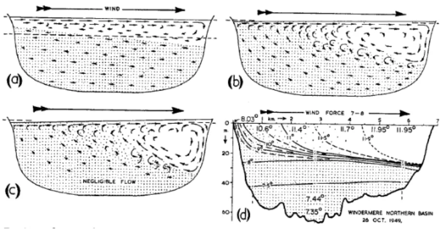
of the metalimnion, it flows back in a direction opposite to the wind (Fig.2.5, Mortimer 1974). The metalimnion is tilted in the process. When the wind stops blowing, the tilted metalimnion is released and adjusts through the generation of basin-scale internal waves. In general the response of the metalimnion to an imposed wind stress is a complex function of geometry, stratification, and the temporal dynamics of the wind forcing (Monismith 1986). For simply shaped and small-to-medium sized lakes, modal-type responses are usually observed (Rao 1966).

Figure 2.5: Two-dimensional representation of the effects of wind on a stratified lake: (a) to (c) stages in the development of the epilimnetic wedge and of shear instability at the downwind end of the thermocline; (d) isotherm distribution in Windermere, northern basin, after about 12 hours of relatively steady wind (fromMortimer 1974).

The Rossby number is a dimensionless number used to characterize the importance of Coriolis effects generated by the Earth rotation (Kundu and Cohen 2004). It is a ratio of inertia to Coriolis terms

Ro= U

2_/L

f U =

U

f L, (2.18)

where f is the Coriolis parameter, and U and L are characteristic velocity and length of

(42)

Figure 2.6: A long Kelvin wave in a uniform depth model (from Mortimer 1974). which length Coriolis effects become important,

R= c

f, (2.19)

wherec is the non-rotating phase speed. R is classified as the external or internal Rossby

radius of deformation for barotropic and baroclinic motions respectively. For small lakes the effect of Earth’s rotation is negligible. The baroclinic motions are then mostly standing waves. The internal waves can be characterized by numbers (modes) indicating the number of the wave nodes in the horizontal and the vertical. When the lake dimension is larger than the internal Rossby radius, the Coriolis effects cannot be neglected. The effect of rotation changes the characteristics of basin-scale internal waves. The wave crests begin to propagate around the boundaries of the lake. The modified long gravity waves usually appear in two different forms: Kelvin waves and Poincaré waves (Wetzel 2001). Kelvin

(43)

the waves travel along the shore of basins in a counterclockwise direction in the northern hemisphere (clockwise in the southern hemisphere). In large lakes long gravity waves can travel in open water without the interference of shore boundaries. Influenced by rotation, these long waves, named Poincaré waves, form a wave pattern of alternating hills and valleys with corresponding cellular patterns of currents (Fig, 2.7, Wetzel 2001). In the northern hemisphere, they have clockwise rotating structures with maximum velocities in the centre. Both types of waves have been observed and studied in many large lakes including Lake Biwa (Saggio and Imberger 1998), Lake Kinneret (Hodges et al. 2000), and Lake Erie (Bouffard et al. 2012).

(44)

Figure 2.7: A standing Poincaré wave in a wide, rotating channel of uniform depth (from

(45)

Chapter

3

Hydrodynamic and Biochemical

Modelling in Lake Erie

In this chapter the coupled ELCOM-CAEDYM is utilized to conduct hydrodynamic and biochemical modelling in Lake Erie. In Section 3.1 the meteorological forcing data are compared and analyzed, and the numerical model is set up in detail in Section3.2. In Section 3.3 the numerical model is validated using field data collected in 2008, via water temperature, currents, and dissolved oxygen. Section3.4demonstrates another application of the ELCOM modelling, where an attempt to explain the 2012 Lake Erie fish kill from a hydrodynamic point of view is proposed.

3.1

Meteorological data process

Lake Erie has three major physiographic divisions: the western, central, and eastern basins. The western basin is the shallowest, with average and maximum depths of 7.4 and 18.9 m. The central basin has average and maximum depths of 18.5 and 25.6 m. It is separated from the western basin by a chain of islands and Point Pelee, and from the

(46)

The eastern basin is the deepest with a mean depth of 24.4 m and a 64.0 m maximum (Bolsenga and Herdendorf 1993). Water levels vary by about0.5m on seasonal time scales. The Detroit river provides about95% of the inflow to Lake Erie at the western end of the western basin. This water then passes through the flat central basin, the bowl-shaped eastern basin, and is finally drained through the Niagara River. The residence time of Lake Erie is about2.6years (O’Sullivan and Reynolds 2004).

In 2008 an intensive field investigation was carried out to gather new information about the meteorology, water temperature, currents, dissolved oxygen, and nutrients in Lake Erie. This field program was part of a project funded by a Strategic Project Grant awarded by the Natural Sciences and Engineering Research Council (NSERC). Ship time was cour-tesy of Environment Canada (National Water Research Institute) and Ontario Ministry of Natural Resources (Wheatley). We thank Ram Yerubandi from NWRI and the crews of these vessels for support in the field. Some of the data used in this study were obtained from Environment Canada, the Great Lake Environmental Research Laboratory, and the National Data Buoy Center.

This section compares available observational meteorological data and prepares the environmental forcing input for ELCOM-CAEDYM, namely, solar and longwave radiation, air temperature, wind, and relative humidity.

3.1.1

Available dataset

There are two sets of observational data available. The first is available from the National Water Research Institute (NWRI) of Environment Canada (EC) and the second from the United State National Data Buoy Center (NDBC) of the National Oceanic and Atmospheric Administration (NOAA). The locations of all available stations are marked in Fig. 3.1. The deployment details at NWRI meteorological stations in 2008 are listed

(47)

over the North American region (Mesinger et al. 2006). It covers 1979 to near present and is provided 8-times daily on a Northern Hemisphere Lambert Conformal Conic grid (32 km in the horizontal and 45 vertical layers).

Most of the NDBC stations are on the coast, but NWRI buoys were deployed off shore. Schwab and Morton (1984) found that the wind speeds from over-land stations need adjustments in order to accurately approximate the over-lake wind speeds. Moreover, the NWRI buoys also recorded the solar and longwave radiation data which were not measured by NDBC stations. Therefore the NWRI buoy data are chosen over NDBC data if available in the desired locations.

Table 3.1: Deployment details at meteorological stations by NWRI in 2008

Station latitude (N), longitude (W) Deployment time (GMT) Sampling interval Air tem-perature sensor height Wind sensor height Components 341 41-47-40, 82-17-35

May 1 - Oct 15 10 min 3.5m 3.5m wind, air temperature, solar and longwave radiation, and relative humidity

Stanley 42-28-00, 81-13-00

Mar 18 - Dec 4 1 hour 5.0m 5.0m wind and air temperature

Colborne 42-44-12, 79-17-24

Mar 14 - Dec 4 1 hour 5.0m 5.0m wind and air temperature

452 42-34-55, 79-55-23

N.A. in 2008, has 2009 data

10 min 3.5m 3.5m wind, air temperature, solar and longwave radiation, and relative humidity

3.1.2

Data comparison

In this sub-section the available observational data are compared and analyzed. The methods to generate input files required by ELCOM-CAEDYM are described, to be spe-cific, solar and longwave radiation, relative humidity, air temperature, and wind.

Solar radiation

(48)

Stanley Colborne EC 341 SBIO1 THLO1 EC 452 THRO1 HHLO1 MRHO1 CNDO1 OWXO1 FAIO1 GELO1 CBLO1 DBLN6 PSTN6 BUFN6

Figure 3.1: Available meteorological stations in Lake Erie from both NWRI (maple leaf) and NDBC (star). The elevation and bathymetry map is from the NOAA Great Lakes Environmental Research Laboratory (GLERL).

(49)

and EC452, which are more than 200 km apart, have solar radiation recorded in 2009. Therefore we can compare the measurements at two stations along with the NARR simu-lated data to investigate how accurate the approximation will be. Notice that EC data are cumulative for 10 mins with the unit KJ m−2_{, so it needs to be converted to SI units W}

m−2_{, using 1 (KJ m}−2₎_/_{600 s = 1000}_/_{600 W m}−2_{. Figure} _3.2 _{compares three sets of data}

from day 185 to 200. Solar radiation has a clear on and off pattern due to the sunrise and sunset every day. In Fig. 3.2(A) EC452 and EC341 data are very similar, indicating that the solar radiation is nearly uniform across the lake. Hence it is reasonable to use one set of data for the whole lake. Figure 3.2(B) compares EC452 and NARR data generated at the same location, and the agreement is satisfactory. Therefore NARR solar radiation will be used to “fill in” when the field observational data are not available.

Figure 3.2: Solar radiation comparison in 2009 at: (A) EC452 and EC341, and (B) EC452 and NARR.

Longwave radiation

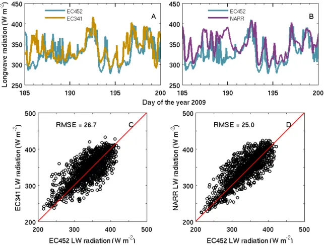
The measurements of downward longwave radiation are in the same situation as those for the solar radiation, namely that the measurements are only available at EC341 in 2008. Figure 3.3 compares the three sets of data again. The agreement is not as good as in the case of solar radiation, but they do follow a similar trend and have comparable

(50)

27 W m−2. The longwave radiation is in the range between 250 and 450 W m−2, so it

is reasonable to assume that data from EC341 can be used to represent the whole lake. The NARR prediction at EC452 agrees well with the observations (Fig.3.3(B,D)), and the RMSE is only 25 W m−2_{. Therefore the NARR data for longwave radiation should also}

be trustworthy when the field data are not available.

Figure 3.3: Downward longwave radiation comparison in 2009 at: (A,C) EC452 and EC341, and (B,D) EC452 and NARR.

(51)

Relative humidity

The relative humidity data were again only measured at EC341 in 2008. Unlike solar and longwave radiation, the relative humidity depends more on local air temperature and pressure, so data from EC452 and EC341 are not expected to be in good agreement, which is shown in Fig. 3.4(A). The NARR prediction is fairly close to the field data at EC452 between day 185 and 200 in Fig. 3.4(B); however, NARR has a warmer bias in air temperature (discussed in the following sub-section). The relative humidity strongly depends on the air temperature, so NARR data should not be used unless there are no field data at all. Hence the dataset from EC341 (the only one available) is chosen for the whole lake in the model setup.

Figure 3.4: Relative humidity comparison in 2009 at: (A) EC452 and EC341, and (B) EC452 and NARR.

Air temperature

Air temperature observations are available from all stations but measured at different heights. Unlike winds, air temperature does not vary much in a few metres above the ground. Therefore, all the air temperature data can be treated at a standard height, say 3.5 m which is the sensor height at EC341.

(52)

Figure3.5plots the air temperature at EC341 and EC Colborne in 2008 and the NARR generated data at the same locations. The NARR data are clearly warmer at both stations through the whole season. In Fig.3.5(C,D) the data distribution has a strong bias towards the NARR side and the RMSE is about2.2◦C at EC341 and2.5◦C at EC Colborne, which are not negligible in both cases. This warmer air temperature bias has been previously mentioned in the literature (e.g. Bennington et al. 2010).

Figure 3.5: Air temperature comparison in 2008 at: (A,C) EC341 and NARR, and (B,D) EC Colborne and NARR.

(53)

Wind

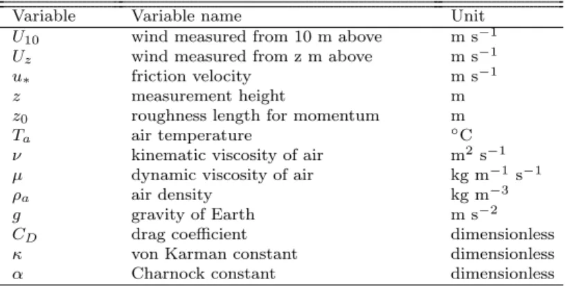
Wind speeds and directions were recorded at all available stations. Similar to the air temperature situation, different stations have various anemometer heights, ranging from 5 to 26 m above the ground (or water). The different measurement heights will significantly affect wind speeds, so we need to convert the wind data to a standard height of 10 m. The conversion method follows Verburg and Antenucci (2010). There is no such method to adjust the wind directions, so they are assumed to remain unchanged in the conversion process.

Table3.2lists all the variables and constants that will be used in the conversion process. First estimate U10 by

u10guess =Uz(10/z)1/7. (3.1) Then the friction velocity is initialized by

u∗guess =u10guess 0.0015 1 +exp(−u10guess+ 12.5 1.56 ) −1 + 0.001041/2. (3.2)

The roughness length for momentum is given by

z0 =αu2∗/g+ 0.11ν/u∗, (3.3) whereν is the kinematic viscosity defined as

ν=µ/ρa. (3.4)

The dynamic viscosity of air is

µ= 4.94×10−8Ta+ 1.7184×10−5. (3.5) There is not enough information to calculate the air density exactly, so it is estimated by the empirical relation between density and temperature. From z0 the friction velocity is

(54)

obtained

u∗ = (CDUz2)1/2 =κUz[ln(z/z0)]. (3.6)

Next loop over (3.3) and (3.6) until z0 is within 0.001% of the previous value of z0. After

obtaining z0 the wind speeds at 10 m height can be calculated by

U10=Uzln(10/z0)/[ln(z/z0)]. (3.7)

Station SBIO1 (South Bass Island, Ohio, Fig. 3.1) from NDBC had wind speeds mea-sured from 21 m above the ground and EC Colborne had data from 5 m above. Figure3.6

compares the original data in both stations with the converted 10 m data. In general wind is stronger when measured further away from the ground. Smaller wind speed values are not affected much by the measurement height, but when the wind speed is larger than 10 m s−1_{, the difference becomes noticeable.}

Table 3.2: A list of variables used in converting wind speeds to 10 m height

Variable Variable name Unit

U10 wind measured from 10 m above m s−1

Uz wind measured from z m above m s−1

u∗ friction velocity m s−1

z measurement height m

z0 roughness length for momentum m

Ta air temperature ◦C

ν kinematic viscosity of air m2 _s−1

µ dynamic viscosity of air kg m−1 _s−1

ρa air density kg m−3

g gravity of Earth m s−2

CD drag coefficient dimensionless

κ von Karman constant dimensionless

(55)

Figure 3.6: (A) EC Colborne wind speeds comparison at 5 m and 10 m above, and (B) NDBC SBIO1 wind speeds comparison at 21 m and 10 m above.

(56)

3.1.3

Summary

In this section the meteorological forcing data from the field observations are compared and analyzed. (i) Solar radiation is almost uniform at two measurement stations 200 km apart in 2009, which indicates very little variation in the horizontal. Hence it is reasonable to use one set of data for the whole lake. The NARR data is compared with EC452 and the agreement is quite good as well. Therefore the NARR outputs can be used to “fill in” solar radiation forcing if the observational data are not available. (ii) The situation for downward longwave radiation is similar. Two sets of field data from Environment Canada in 2009 show reasonable agreement, and the NARR prediction is considered acceptable as well. Hence one set of data for can be used for the whole lake and NARR data are adequate to estimate if needed. (iii) Unlike solar and longwave radiation, the relative humidity strongly depends on local air temperature and pressure, and the comparison of two sets of field data in 2009 confirms it. Unfortunately there is only one dataset containing the relative humidity measurement in 2008. Although NARR does provide the desired data, the warmer bias in the air temperature makes the NARR data problematic. In the model setup the EC341 relative humidity data are chosen to force the whole lake instead of using NARR data. (iv) It was assumed that temperature variations between 2 and 10 m above the surface are insignificant. The comparison between field data and NARR data at the same location shows an obvious warmer bias in NARR. The RMSE is as large as 2.5◦C through the ice-free season. We should always keep this in mind when dealing with the air temperature in NARR. (v) Finally using the method in Verburg and Antenucci (2010) the wind speeds from various measurement heights are converted to the standard 10 m. The difference in the measurement heights has a larger effect on stronger winds (larger than 10 m s−1).

(57)

3.2

Model setup

Numerical simulations were conducted using ELCOM-CAEDYM (EL-CD). In order to address the spatial variability of meteorological conditions across the lake, the computa-tional domain was divided into four sections: the eastern, east-central, west-central, and western (Fig 3.7). In each section the environmental forcing was set to be uniform and equal to the observational data at the nearby station, i.e., Port Colborne in the eastern section, Port Stanley in the east-central, and station 341 in the west-central. Due to in-sufficient field data in the western basin from NWRI, data from station SBIO1 at NDBC were used instead. Only the buoy at station 341 recorded solar and longwave radiation and relative humidity, so these values are used over the whole lake. Data from station 341 were only available from May 2 to October 15 so data from NDBC and reanalysis NARR were used for the time periods from April 21 to May 2 and Oct 16 to 30. The time series of 3-hour averaged meteorological data at station 341 is plotted in Fig.3.8.

Inflow from eleven major tributaries to Lake Erie (Detroit, Raisin, Maumee, Sandusky, Vermilion, Rocky, Cuyahoga, Grand [Ohio, USA], Cattaraugus, Buffalo and Grand [On-tario, Canada]) was included in the study. The Detroit River, which is the largest inflow, and ten other inflows together account for 99.7% of all lake inflows. The remaining tribu-taries have negligible impact on the lake’s physical dynamics or heat budget. Lake water is drained through the Niagara River to Lake Ontario. The data on flow rates and water temperatures for the modelled tributaries were obtained by Dr. Serghei Bocaniov from several datasets that included the US Geological Service, the US EPA database on water quality monitoring data (STORET), Water Survey of Canada from Environment Canada and Grand River Conservation Authorities (GRCA, Ontario).

Processing the river data and the CAEDYM setup were performed by Dr. Serghei Bocaniov, formerly in the Department of Biology at the University of Waterloo, along with Professor Ralph Smith and their colleagues. CAEDYM simulates the C, N, P, DO, and Si cycles, along with inorganic suspended solids and phytoplankton. Twelve state variables are required to model the algal biomass. Five dissolved inorganic nutrients (PO , NO ,

(58)

Stanley Colborne 341 1227 1228 1231 84 357 SBIO1 452

Figure 3.7: Lake Erie bathymetry (from GLERL) with four forcing sections (divided by dash lines) and the locations of meteorological buoys (N) and thermistor chains ( ).

(59)

Figure 3.8: Time series of 3-hour averaged meteorological data at station 341: (A) air temperature, (B) solar radiation, (C) downward longwave radiation, (D) relative humidity, and (E) wind speed (lines) and wind direction (dots, measured clockwise from north in direction wind is coming from).

(60)

detrital organic matter groups (POC, PON, and POP), two inorganic suspended solids size classes (SS1 and SS2), and dissolved oxygen (DO) were simulated.

The Lake Erie bathymetry was obtained from the Great Lake Environmental Research Laboratory (GLERL). The computational grid used a 2 km horizontal resolution and 45 unevenly spaced vertical layers with thicknesses varying between 0.5 to 5 m. The simula-tions started with the lake at rest with the water temperature initialized with observational data from mooring stations, which is then horizontally interpolated using the inverse dis-tance weighting method (ELCOM User Manual 2006). The typical spin up time of the lake circulation is relatively short, largely because of the shallow depth of the lake and the strong wind-driven character of the lake hydrodynamics (Beletsky and Schwab 2001). Therefore, the effect of initial conditions on the seasonal scale is negligible after a few weeks. A mixed-layer turbulence scheme and a drag parametrization along the bottom and side boundaries was applied. The model runs for a period of 193 days, from April 21 to October 30 with a 5-minute time step, which is used to achieve both numerical stability and a reasonable completion time. A seasonal ELCOM simulation takes about 13 physical hours to finish using one 3.0 GHz Intel Xeon processor, and a coupled EL-CD run takes approximately seven times longer.

3.3

Model validation

In the 2008 field investigation seven temperature logger chains with a 10-minute sam-pling interval were deployed at stations 357, 1227, 1228, 1231, 341, 84, and 452 (Fig.3.7). Three high frequency data sets with a 10-second sampling time interval were recorded at stations 1227, 1228, and 1231 as well. One Acoustic Doppler Current Profiler (ADCP) was set at station 341. The deployment details are listed in Table 3.3. In addition, the lake surface temperature averaged over the Great Lakes derived from satellite remote sensing

(61)

2005; Leon et al. 2011). In this section another model validation in a different year is provided to confirm its modelling ability to capture the lake dynamics. The ability of the model to simulate quantities of interest is quantified by calculating the root mean square error (RMSE) and average percentage difference (APD):

RMSE= 1 M M X i=1 (f_im−f_io)21/2, (3.8) APD= 1 M M X i=1 fm i −fio fo i ×100%, (3.9) where fm

i and fio are modelled and observed quantities for sample case i out of M cases (Huang et al. 2010a).

Table 3.3: Deployment details at mooring stations by NWRI in 2008

Station latitude (N), longitude (W) Depth (m) Type Deployment time (GMT) Sampling interval (min) Depth of measurement (m)

357 41-49-59, 82-57-03 10.1 Temperature May 1 - Oct 14 10 [1 3 5 7 9]

1227 41-48-36, 82-30-09 11.5 Temperature Jun 3 - Oct 15 10 [1 2 3 4 6 7 8 8.7 9.2 11]

1228 41-47-40, 82-21-13 14.5 Temperature Jun 4 - Oct 15 10 [1 2 3 5 6 7 8 11.5 12 12.5 13 13.5] 1231 41-47-30, 82-11-38 19.8 Temperature Jun 3 - Oct 15 10 [1 2 3 4 5 6 7 8 10 11.5 12.5 13 14

15 15.5 16 16.5]

341 41-47-40, 82-17-35 17.6 Temperature May 2 - Oct 14 15 [1 2 3.5 4.5 5.5 6.5 7.5 8.5 9.5 12.75 13.5 14.5 15 15.5 15.9 16.5 17] 341 41-47-40, 82-17-35 15.3 ADCP Apr 28 - Nov 8 15 [1 2 3 4 5 6 7 8 9 10 11 12 13 14 15] 84 41-55-07, 81-38-46 23.6 Temperature Apr 29 - Oct 16 10 [1 3 5 7 9 11 13 15 16 17 18 19 20

21 22 23]

452 42-34-55, 79-55-23 53.5 Temperature Apr 29 - Oct 16 10 [1 3 5 7 9 11 13 15 16 17 18 19 20 23 26 30 35 40 45 50]

3.3.1

Water temperature

Temperature determines the solubility of many substances, influences organism distri-butions based on thermal habitat preferences (e.g. Lynch et al. 2010), and affects the rate of chemical reactions and biological processes such photosynthesis and respiration (Falkowski and Raven 2007).

(62)

Figures 3.9 and 3.10 compare the observed and modelled temperature time series at several different locations. (i) At station 357 the numerical model successfully predicts the heating of the lake in the spring and summer and cooling in the fall (Fig. 3.9(A,D,J)). Station 357 is located in the shallowest western basin where the stratification is very weak, so the excellent agreement is not surprising. (ii) Moving eastwards to station 1227 in the central basin, the lake becomes slightly deeper (11.5 m) and is only weakly stratified near the bottom in the summer. The model correctly captures the stratification but with slightly warmer predictions (Fig.3.9(B,E,H,K)). (iii) At station 341 (Fig.3.9(C,F,I,L)) and 1231 (Fig.3.10(A,D,G,J)) the stratification becomes stronger and lasts longer. The model captures the seasonal evolution; however, the water temperature is overestimated in the summer, and the predicted metalimnion is deeper and thicker. The modelled metalimnion is thicker than observed due to numerical diffusion and this is a known problem of all current hydrodynamic models (Huang et al. 2010b). Moreover it also may be caused by the weaknesses of the mixing parametrization in ELCOM. Around day 210 (July 28) a strong storm was believed to emerge near station 1231, which is indicated in the obser-vational data by the colder 10◦_{C water that appears at depths between 6 to 10 m. This} cooling event was not simulated by the model, probably because the s