An aly si s fo r F o r e c a s ti n g
Ty p e
Ar ticl e
U RL
h t t p s :// u al r e s e a r c h o nli n e . a r t s . a c . u k/i d/ e p ri n t/ 1 5 6 4 8 /
D a t e
2 0 2 0
Cit a ti o n
H a s s a n i, H . a n d Yeg a n e g i, M . R. a n d Kh a n , A. a n d Silv a,
E . S. ( 2 0 2 0 ) T h e Eff e c t of D a t a T r a n sf o r m a ti o n o n Si n g u l a r
S p e c t r u m An aly si s fo r F o r e c a s ti n g . Si g n a l s, 1 ( 1). IS S N
2 6 2 4-6 1 2 0
C r e a t o r s
H a s s a n i, H . a n d Yeg a n e g i, M . R. a n d Kh a n , A. a n d Silv a,
E . S.
U s a g e G u i d e l i n e s
Pl e a s e r ef e r t o u s a g e g u i d eli n e s a t
h t t p :// u al r e s e a r c h o n li n e . a r t s . a c . u k / p olici e s . h t m l
o r a l t e r n a tiv ely c o n t a c t
u a l r e s e a r c h o n li n e @ a r t s . a c . u k
.
Lic e n s e : C r e a tiv e C o m m o n s Att ri b u ti o n N o n-c o m m e r ci al N o D e riv a tiv e s
U nl e s s o t h e r wi s e s t a t e d , c o p y ri g h t o w n e d b y t h e a u t h o r
Article
The Effect of Data Transformation on Singular
Spectrum Analysis for Forecasting
Hossein Hassani1,*,† , Mohammad Reza Yeganegi2,† , Atikur Khan3,† and Emmanuel Sirimal Silva4,†
1 Department of Business & Management, Webster Vienna Private University, 1020 Vienna, Austria
2 Department of Accounting, Islamic Azad University, Central Tehran Branch, Tehran 477893855, Iran;
3 Qantares, 97 Broadway, Nedlands 6009 (Perth), Western Australia, Australia; [email protected]
4 Centre for Fashion Business and Innovation Research, Fashion Business School, London College of Fashion,
University of the Arts London, London W1G 0BJ, UK; [email protected]
* Correspondence: [email protected]
† These authors contributed equally to this work.
Received: 14 January 2020; Accepted: 17 April 2020; Published: 7 May 2020
Abstract: Data transformations are an important tool for improving the accuracy of forecasts from time series models. Historically, the impact of transformations have been evaluated on the forecasting performance of different parametric and nonparametric forecasting models. However, researchers have overlooked the evaluation of this factor in relation to the nonparametric forecasting model of Singular Spectrum Analysis (SSA). In this paper, we focus entirely on the impact of data transformations in the form of standardisation and logarithmic transformations on the forecasting performance of SSA when applied to 100 different datasets with different characteristics. Our findings indicate that data transformations have a significant impact on SSA forecasts at particular sampling frequencies.
Keywords:logarithmic transformation; standardisation; forecasting; singular spectrum analysis
1. Introduction
Amidst the emergence of Big Data and Data Mining techniques, forecasting continues to remain an important tool for planning and resource allocation in all industries. Accordingly, researchers, academics, and forecasters alike invest time and resources into methods for improving the accuracy of forecasts from both parametric and nonparametric forecasting models. One approach to improving the accuracy of forecasts is via data transformations prior to fitting time series models. For example, it is noted in [1] that data transformations can simplify the forecasting task, whilst evidence from other research indicates that, in economic analysis, taking logarithms can provide forecast improvements if it results in stabilising the variance of a series [2]. However, studies also indicate that data transformations will not always improve forecasts [3] and that they could complicate time series analysis models [4,5].
In fact, a key challenge for forecasting under data transformation is to transform the data back to its original scale, a process which could result in a forecasting bias [6,7]. Historically, most studies have focused on the impact of data transformations on parametric models such as Regression and Autoregressive Integrated Moving Average (ARIMA) models [8,9]. More recently, authors have resorted to evaluating the impact of data transformations on several other forecasting models [10,11], further highlighting the relevance and importance of the topic. Our interest is focused on the evaluation of the impact of data transformations on a time series analysis and forecasting technique called Singular Spectrum Analysis (SSA).
In brief, the SSA technique is a popular denoising, forecasting, and missing value prediction technique with both univariate and multivariate capabilities [12,13]. Recently, its diverse applications have focused on forecasting solutions for varied industries and fields, from tourism [14,15] and economics [16–18] to fashion [19], climate [20,21], and several other sectors [22–24]. Regardless of its wide and varied applications, researchers have yet to explore the effect of data transformations on the forecasting performance of this nonparametric forecasting technique. Previously, in [25], the authors evaluated the forecasting performance of the two basic SSA algorithms under different data structures. However, their work did not extend to evaluating the impact of data transformations to provide empirical evidence for future research. Accordingly, through this paper, we aim to contribute to the existing research gap by studying the effects of different data transformation options on the forecasting behaviour of SSA.
Logarithmic transformation is the most commonly used transformation in time series analysis. It has been used to convert multiplicative time series structures to additive structures or to reduce the time series skewness volatility and increase stability [2,26]. The autocorrelation structure in the time series may change under different transformations that may affect the model, and different transformations may result in different specifications for ARIMA models [6,27]. Like ARIMA models, SSA too can be greatly influenced by transformations. For instance, if data transformation makes noise uncorrelated or reduces the complexity of the time series, it can improve SSA performance [21,26]. As data standardisation and logarithmic transformations are the easiest in terms of interpretability and back-transformation to the original scale, we explore the effect of these data transformations on the forecasting performance of SSA.
The remainder of this paper is organised as follows. In Section 2, we provide a detailed exposition of SSA and its recurrent and vector forecasting algorithms. In Section 3, we present data transformation techniques and their effect on forecasting accuracy. Procedures for examining the effect of transformation based on different characteristics of time series are presented in Section4. In Section5, we analyse different datasets of varied characteristics and present our results for an evidence-based exploration of the effect of data transformations on SSA forecasts. Finally, we present our concluding remarks in Section6.
2. SSA Forecasting
There are two different algorithms for forecasting with SSA, namely recurrent forecasting and vector forecasting [12,28]. Those interested in a comparison of the performance of both algorithms are referred to [25]. Both of these forecasting algorithms require that one follows two common steps of SSA, the decomposition and reconstruction of a time series [12,28]. In what follows, we provide a brief description of forecasting processes in SSA.
2.1. Decomposition and Reconstruction of Time Series
In SSA, we embed the time series{x1,x2, . . . ,xN}into a high-dimensional space by constructing a Hankel structured trajectory matrix of the form:
X= x1 x2 x3 . . . xn x2 x3 x4 . . . xn+1 .. . ... ... . . . ... xm xm+1 xm+2 . . . xN = [x1 . . . xi . . . xn], (1)
wheremis the window length, them−lagged vectorxi = (xi,xi+1, . . . ,xi+m−1)0is theith column of
The singular value decomposition (SVD) of the trajectory matrixXcan be expressed as X=Sk+Ek= k
∑
j=1 q λjujv0j+ m∑
j=k+1 q λjujv0j (2)whereujis thejth eigenvector ofX X0corresponding to the eigenvalueλjandvj =X0uj/
q
λj. Ifkis the number of signal components,Sk =∑kj=1
q
λjujv0jrepresents a matrix of signal, and
Ek = ∑mj=k+1
q
λjujv0j is the matrix of noise. We apply the diagonal averaging procedure toSk to reconstruct the signal seriesxetsuch that the observed series can be expressed as
xt=ext+eet, (3)
wherexetis the less noisy, filtered series. A detailed explanation of decomposition in Equation (3) can
be found in [28,29].
To construct the trajectory matrixXin Equation (1) and to conduct the SVD in Equation (2), we have to select the Window Lengthmand the number of signal componentsk. Since our aim is not to demonstrate the selection of SSA choices (mandk), we opt not to reproduce the selection procedures for SSA choices, as these are already covered in depth in [12,28]. As our interest is in examining the effect of transformation on the forecasting performance of SSA, we selectmandksuch that the Root Mean Squared Error (RMSE) in forecasting is minimised.
2.2. Recurrent Forecasting
Recurrent forecasting in SSA is also known asR-forecasting, and the findings in [25] indicate that R-forecastingis best when dealing with large samples. Ifu∇j = (u1j, . . . ,u(m−1)j)0is the vector of the firstm−1 elements of thejth eigenvectoruj, andumjis the last element ofuj. The coefficients of linear recurrent equation can be estimated as
a= (a(m−1), . . . ,a1)0= 1 1−∑k j=1u2mj k
∑
j=1 umju∇j . (4)With the parameters in Equation (4), a linear recurrent equation of the form
e xt= m−1
∑
i=1 a(m−i)ext−m+i (5)is used to obtain a one-step-ahead recursive forecast [29]. This linear recurrent formula in Equation (5) is used to forecast the signal at timet+1 given the signal at timet,t−1, . . . ,t−m+2 [28] (Section2.1, Equations (1)–(6)), and the one-step-ahead recursive forecast ofxN+jis
ˆ xN+j = ( ∑ij=−11aixˆN+j−i+∑m −j i=1 am−iexN+j−m+i forj≤m−1; ∑m−1 i=1 aixˆN+j−i forj>m−1. (6) We apply the recursive forecasting method in Equation (6) to obtain a one-step-ahead forecast. 2.3. Vector Forecasting
In contrast, the SSA Vector forecasting algorithm has proven to be more robust than the R-forecastingalgorithm in most cases [25]. Let us defineU∇k =
u∇1 . . . u∇k
as the(m−1)×kmatrix consisting of the firstm−1 elements ofkeigenvectors. The vector forecasting algorithm computes
m−lagged vectors ˆzi and constructs a trajectory matrix Z = [zˆ1 . . . zˆn zˆn+1 . . . zˆn+h] such that ˆ zi = si fori=1, 2, . . . ,n; U∇kU∇k0+ (1−∑k j=1u2mj)aa0 ˆ z4i−1 a0zˆ4i−1 ! fori=n+1, . . . ,n+h. (7)
wheresi is theith column of the reconstructed signal matrixSk =∑kj=1
q
λjujv0j, and ˆz
4
i is the last
m−1 elements of the vector ˆzi.
After a diagonal averaging of the matrix Z = [zˆ1 . . . zˆn zˆn+1 . . . zˆn+h] constructed by employing Equation (7), we obtain a time series{zˆ1, . . . , ˆzN, ˆzN+1, . . . , ˆzN+h}, as has also been explained in [28] (Section 2.3) . Thus, ˆxN+j = zˆN+j produces a forecast corresponding toxN+j for
j=1, . . . ,h.
3. Transformation of Time Series
Data transformation is useful when the variation increases or decreases with the level of the series [1]. Whilst logarithmic transformation and standardisation are the most commonly used data transformation techniques in time series analysis, it is noteworthy that there are other transformations from the family of power transformation such as square root and cube root transformations. However, the interpretability is not as simple and common as that for standardisation and logarithmic transformation.
3.1. Standardisation
Standardisation of time series{xt}is formulated as
yt= xt −x¯
σx , (8)
where ¯x and σx are the mean and standard deviation of the series {xt}, respectively. Data standardisation is another common data transformation in preprocessing. Standardisation is mostly common in machine learning techniques to reduce training time and error. In time series forecasting, standardisation has proven advantages when we are using machine learning algorithms (e.g., neural networks and deep neural networks) [30]. In terms of SSA, the theoretical literature does not investigate the effect of standardisation on SSA forecasts in detail. However, in Golyandina and Zhigljavski [26], the authors addressed the effect of centering the time series as preprocessing. In theory, if the time series can be expressed as an oscillation around a linear trend, centering will increase the SSA’s accuracy [26].
3.2. Logarithmic Transformation
In this paper, the following logarithmic transformation is applied on time series{xt}:
yt=log(C+xt), (9)
whereCis a constant value, large enough to guarantee that the term inside the logarithm is positive. As mentioned before, log-transform is a common preprocessing to handle variance instability or right skewness. Furthermore, one may use log-transform as a form of preprocessing to convert a time series with a multiplicative structure to an additive one. Given that SSA can be applied to time series with both additive and multiplicative structures, it does not necessarily need log-transform pre-processing [26]. However, the authors in Golyandina and Zhigljavski [26] showed that using log-transform could affect SSA’s forecasting accuracy. In fact, SSA’s forecasting accuracy will increase if the rank of a transformed series is smaller than the original one.
4. Comparison between Transformations
Time series with different characteristics will behave differently after transformation. For instance, forecasting accuracy in time series, with positive skewness, non-stationarity, and non-normality, may improve with logarithmic transformation. Furthermore, in time series with large observations or large variance, standardisation can improve the forecasting accuracy. Sampling frequency is another potential factor affecting forecasting accuracy. Time series with high sampling frequency (e.g., hourly or daily) usually have an oscillation frequency close to its noise frequency and consequently show instable and noisy behaviour. On the other hand, time series with larger sampling frequency are smoother. These characteristics of time series may affect forecasting and accuracy as well. As such, to investigate the practical effect of data transformation in SSA forecasting, we should consider “Sampling Frequency,” “Skewness,” “Normality,” and “Stationarity” as control factors.
To observe the effectiveness of data transformation prior to the application of SSA, we may compare the forecasting performance of SSA under different transformations and control factors: firstly, by comparing the Root Mean Squared Forecast Error (RMSFE), and secondly, by employing a nonparametric test to examine the treatment effect (data transformation).
4.1. Root Mean Squared Forecast Error (RMSFE)
The most commonly adopted approach for comparing the predictive accuracy between forecasts is to compute and compare the RMSFE from out of sample forecasts. The RMSFE can be defined as
RMSEh= v u u t1 h N+h
∑
t=N+1 (xt−xˆt)2, (10)wherehis the forecast horizon, N is the number of observations,xtis observed value of time series, and ˆxtis the forecasted value.
The application of data transformation prior to forecasting with SSA may significantly affect the forecasting outcome and the affect may vary based on the properties of a time series. Thus, we need to examine the effect of data transformation on RMSFE along with the differing properties of time series. Comparisons between the RMSFE of the original and transformed time series can be used to learn about the forecasting performance of a model for a given time series. However, comparison of RMSFE for a pool of time series with different characteristics is not straightforward. We compute RMSEhforh=1, 3, 6, 12 (h=1 for a short-term forecast,h=12 for a long-term forecast, andh=3, 6 as a medium-term forecasting horizon) for each of the time series in the pool and examine the effect of transformation by using statistical tests.
4.2. Nonparametric Repeated Measure Factorial Test
Treatment effects in the presence of factors can be examined by employing the nonparametric repeated measure factorial test [31,32] for a pool of time series of different characteristics. Thus, the effect of data transformation (treatment) can be examined by using this test under different characteristics of a time series.
Let us assume that we haveKtime series in the pool with series codeAk, k=1, . . . ,Kand for each of the seriesRMSEhforh=1, 3, 6, 12 are computed. If the interest lies on exploring the effect of transformation for the skewness property of time series, we essentially perform the test for treatment effect (transformation) for categories of skewness properties of these time series. There are three factor levels of the factor Skewness, namely Skew Negative, Skew Positive, and Skew Symmetric. Similarly, we will have two levels for the factor Normality (Yes = normal; No = not normal) and two levels for the factor Stationarity (Yes = stationary; No = nonstationary). To test the effect of transformation (No transformation, Standardisation, and Logarithmic transformation), we follow the procedures described below.
First, we learn some basic characteristics of a time series such as normality, stationarity, skewness, and frequency. For example, the frequency of a time series can be learnt by examining the time of measurement: hourly, daily, weekly, monthly, or annually. We also classify time series into different categories via a series of statistical tests such as the Jarque-Bera test for normality [33], the KPSS test for stationarity [34], and the D’Agostino test for skewness [35].
Secondly, the nonparametric repeated measure factorial test [31,32] is used to test the effect of the transformation on RMSFE, across different categories where categories are defined based on Frequency, Normality, Skewness, and Stationarity.
5. Data Analysis
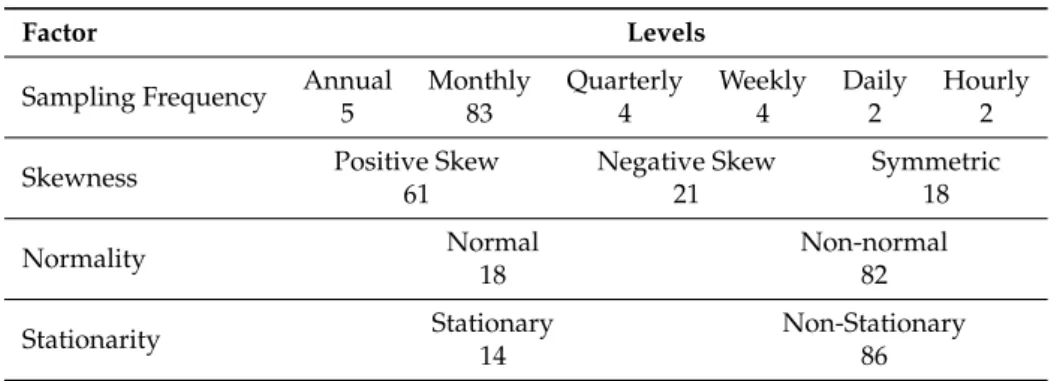
We used the same set of time series employed by Ghodsi et al. [25] to test the effect of data transformation on SSA forecasting accuracy, with different characteristics. The dataset contains 100 real time series with different sampling frequencies and stationarity, normality, and skewness characteristics, representing various fields and categories, obtained via the Data Market (http:// datamarket.com). Table1presents the number of time series with each feature. It is evident that the real data includes data recorded at varying frequencies (annual, monthly, weekly, daily, and hourly) alongside varying distributions (normal distribution, skewed, stationary, and non-stationary). Interestingly, the majority of the data are non-stationary overtime, which resonates with expectations within real-life scenarios.
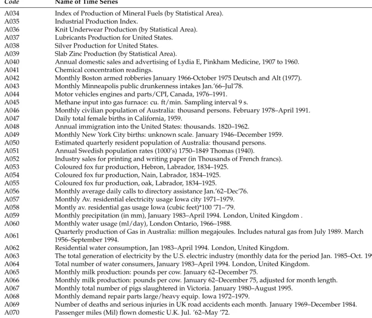
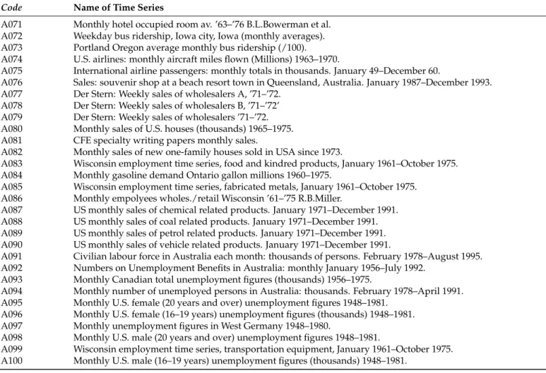
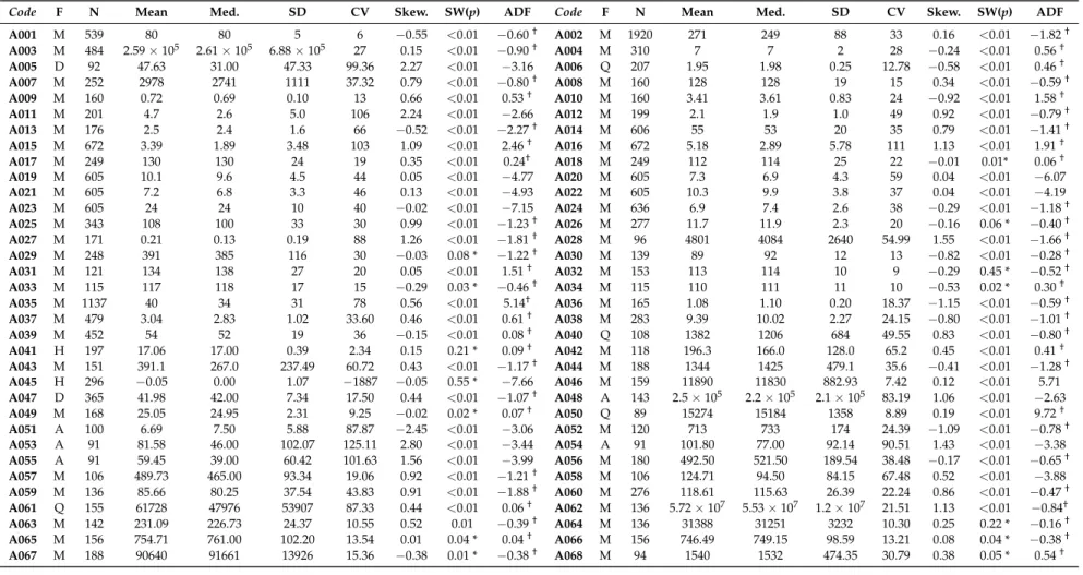
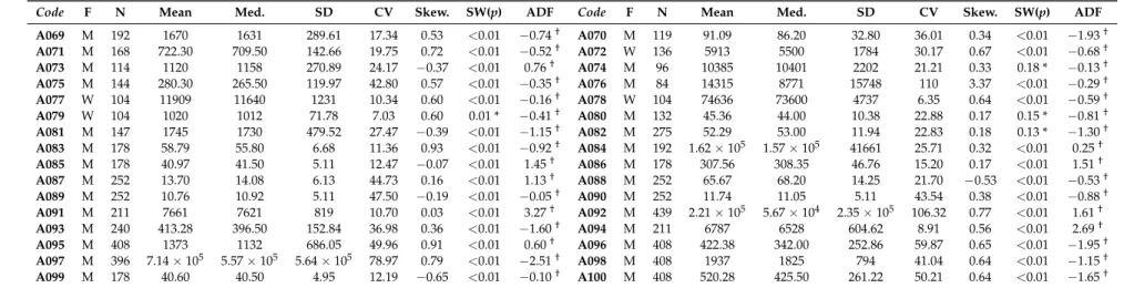
The name and description of each time series and their codes assigned to improve presentation are presented in TableA1. TableA2presents descriptive statistics for all time series to enable the reader to obtain a rich understanding of the nature of the real data. This also includes skewness statistics, and results from the normality (Shapiro-Wilk) and stationarity (Augmented Dickey-Fuller) tests. As visible in TableA1, the data comes from different fields such as energy, finance, health, tourism, housing market, crime, agriculture, economics, chemistry, ecology, and production.
Table 1.Number of time series with each feature.
Factor Levels
Sampling Frequency Annual Monthly Quarterly Weekly Daily Hourly
5 83 4 4 2 2
Skewness Positive Skew Negative Skew Symmetric
61 21 18
Normality Normal Non-normal
18 82
Stationarity Stationary Non-Stationary
14 86
Figure1shows the time series for a selection of 9/100 series used in this study. This enables the reader to obtain a further understanding of the different structures underlying the data considered in the analysis. For example, A007 is representative of an asymmetric non-stationary time series for the labour market in a U.S. county. This monthly series shows seasonality with an increasing non-linear trend. In contrast, A022 is related to a meteorological variable that is asymmetric, yet stationary and highly seasonal in nature. An example of a time series that is both asymmetric and non-stationary is A038, which represents the production of silver. Here, structural breaks are visible throughout. A055 is an annual time series, which is stationary and asymmetric, and relates to the production of coloured fox fur. An example of a quarterly time series representing the energy sector is shown via A061. This time series is non-stationary and asymmetric with a non-linear trend and an increasing seasonality over time. Another example focuses on the airline industry (A075) and is also asymmetric and non-stationary in nature. It appears to showcase a linear and increasing trend along with seasonality. A skewed and non-stationary sales series is shown via A081, with the trend indicating increasing seasonality with
major drops in the time series between each season. A time series for house sales (A082) can be found to be normally distributed and non-stationary over time. It also shows a slightly curved non-linear trend and a sine wave that is disrupted by noise. Finally, the labour market is drawn on again via A094, but this is an example of a time series affected by several structural breaks leading to a non-stationary, asymmetric series, which also has seasonal periods and a clear non-linear trend.
A007 Month W or kf orce 1950 1955 1960 1965 1000 3000 5000 7000 A022 Month Celsius Degrees 1960 1980 2000 0 5 10 15 A038 Month
Millions Of Fine Ounces
1925 1930 1935 1940 1945 2 4 6 8 10 14 A055 Year Fur Production 1840 1860 1880 1900 1920 0 50 150 250 A061 Quarter Millions of Megajoules 1960 1970 1980 1990 0 50000 150000 A075 Month Thousands of P assengers 1950 1954 1958 100 300 500 A081 Month Sales of Wr iting P apers 2002 2006 2010 500 1500 2500 A082 Month House Sales 1975 1980 1985 1990 1995 30 50 70 90 A094 Month Number of P eople 1980 1985 1990 1995 4e+05 7e+05 1e+06
Figure 1.A selection of nine real time series.
R packages “Rssa” [36–38] and “nparLD” [39] are employed to implement SSA forecasting and the nonparametric repeated measure factorial test, respectively. We apply SSA to three versions of a dataset: a dataset without any transformation, a standardised dataset, and a log-transformed dataset. For each of the three datasets, we obtain RMSFE from out-of-sample forecasting at forecast horizons h=1, 3, 6, 12. It is noteworthy that our aim in this paper is to examine the effect of transformation in SSA forecasting. Thus, we consider the best forecast based on the RMSFE of the last 12 data points regardless of whether the forecast is from the recurrent or vector-based approach.
We also know that the window lengthm, the number of componentsk, and the forecasting methods (recurrent and vector) affect the forecasting outcome. Thus, we adopt a computationally intensive approach by considering combinations ofmandk, and methods that provide the minimum RMSFE for the out-of-sample forecast for the last 12 data points. The RMSFEs obtained from the computationally intensive approach are given in TablesA3–A6.
Given that the best forecasting results are achieved by util ising a computationally intensive approach, we seek to identify the factors that can affect the RMSFE. In order to address this, we employ statistical tests described in Section4.2. For each of the series with RMSFE reported in Tables
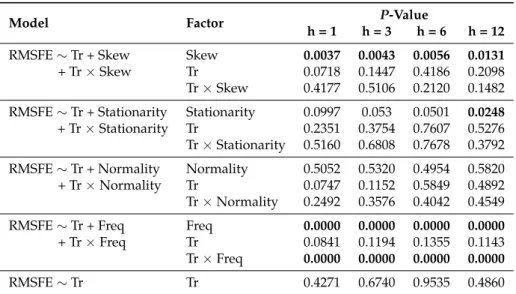
A3–A6, we examine the characteristics of the time series by employing a statistical test, as described in Section4.2. At this stage, we are ready with the inputs for nonparametric repeated measure factorial test to conduct testing on the treatment effect (data transformation) under different characteristics of these time series. Results obtained from the Wald type tests are provided in Table2.
Table 2.Wald-type test results.
Model Factor P-Value
h = 1 h = 3 h = 6 h = 12
RMSFE∼Tr + Skew Skew 0.0037 0.0043 0.0056 0.0131
+ Tr×Skew Tr 0.0718 0.1447 0.4186 0.2098
Tr×Skew 0.4177 0.5106 0.2120 0.1482
RMSFE∼Tr + Stationarity Stationarity 0.0997 0.053 0.0501 0.0248
+ Tr×Stationarity Tr 0.2351 0.3754 0.7607 0.5276
Tr×Stationarity 0.5160 0.6808 0.7678 0.3792
RMSFE∼Tr + Normality Normality 0.5052 0.5320 0.4954 0.5820
+ Tr×Normality Tr 0.0747 0.1152 0.5849 0.4892
Tr×Normality 0.2492 0.3576 0.4042 0.4549
RMSFE∼Tr + Freq Freq 0.0000 0.0000 0.0000 0.0000
+ Tr×Freq Tr 0.0841 0.1194 0.1355 0.1143
Tr×Freq 0.0000 0.0000 0.0000 0.0000
RMSFE∼Tr Tr 0.4271 0.6740 0.9535 0.4860
Here, Freq, Skew, and Tr represent frequency, skewness, and transformation, respectively. Bold values show the significant effects at theα=0.05 significance level.
Based on the Wald-type test results in Table2, we may conclude that, at theα=0.05 significance level,
1. normality does not affect SSA forecasting performance;
2. stationarity affects SSA forecasting performance in long-term forecasting (h = 12) but not at shorter horizons;
3. skewness and sampling (observation) frequency affect SSA forecasting performance;
4. transformation does not affect SSA forecasting performance, but the interaction between sampling frequencies and transformation is significant, which means the SSA performance is affected by transformation at some sampling frequencies.
The above findings are important in the practice for several reasons. First, in the real world, it is well known that most time series do not meet the assumption of normality. However, as the effect of normality and its interactions with transformations are not significant, when faced with normally distributed data, our findings indicate that there is no impact on the forecasting accuracy of SSA with or without data transformations. Furthermore, these findings also indicate that data transformations do not improve the forecast accuracy in non-normal data either. Secondly, we find that, when series are stationary, it affects the long-term forecasting accuracy of SSA. However, when generating short-term forecasts, the forecasting accuracy of SSA is not affected by stationarity. Thirdly, in reality, as most time series are skewed and increasingly found at varying frequencies (especially following the emergence of Big Data), these findings show that forecasters should remember that varying skewness and frequency of data are features indicative of the need for careful exploration of the use of SSA as the forecasts are sensitive to these features. In general, transformations are not required when forecasting with SSA, as there is no evidence of transformations impacting the SSA forecasting performance; however, there could be a significant impact at certain sampling frequencies. This indicates that, when modelling
data with different frequencies, the sensitivity of SSA forecasts to such frequencies could potentially be controlled by transforming the input data.
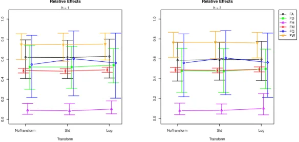
Since the interaction between sampling frequency and transformation is significant, we explore the relative effect of frequencies on RMSFE. Figure2shows the effect plot of treatment (transformation) for different forecast horizonsh=1, 3, 6, 12.
0.47 0.49 0.51 0.53 Relative Effects Transform NoTransform Std Log h = 1 0.47 0.49 0.51 0.53 Relative Effects Transform NoTransform Std Log h = 3 0.47 0.49 0.51 0.53 Relative Effects Transform NoTransform Std Log h = 6 0.46 0.48 0.50 0.52 0.54 Relative Effects Transform NoTransform Std Log h = 12
Figure 2.Effect plot: RMSFE∼Tr.
To explore the relative effects of sampling frequency for different forecast horizons, we plot the relative effect of frequencies in Figures3and4.
0.0 0.2 0.4 0.6 0.8 1.0 Relative Effects Transform NoTransform Std Log h = 1 0.0 0.2 0.4 0.6 0.8 1.0 Relative Effects Transform NoTransform Std Log h = 3 FA FD FH FM FQ FW
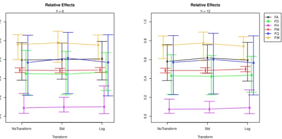
0.0 0.2 0.4 0.6 0.8 1.0 Relative Effects Transform NoTransform Std Log h = 6 0.0 0.2 0.4 0.6 0.8 1.0 Relative Effects Transform NoTransform Std Log h = 12 FA FD FH FM FQ FW
Figure 4.Effect plot: RMSFE∼Tr + Freq + Tr×Freq for forecast horizonsh=6 andh=12.
Sampling frequencies under investigation are hourly (F H), daily (F D), weekly (F W), monthly (F M), and annual (F A). When the relative effect plots in Figures3and4are compared with the effect plots in Figure2, we can evaluate how the hourly (F H), weekly (F W), quarterly (F Q), and annual (F A) sampling frequencies are affecting the forecasting performance of SSA. Moreover, the change in shape of the transform’s relative effects (e.g., see the difference between the shapes of “F Q” and “F H” lines in Figures3and4) suggests an interaction between transformation and sampling frequency.
We analyse the results by forecasting horizon. It can be seen in Figure3that, in very short-term forecasting (h=1), the standardisation produces a comparatively large RMSFE in quarterly frequencies, while the log transformation reports a slightly larger RMSFE at daily, quarterly, hourly, and annual frequencies. This indicates that users should certainly avoid transforming data with quarterly frequencies when forecasting ath = 1 step ahead with SSA. In the short-term forecasting horizon (h=3) (see Figure3), the smallest RMSFE belongs to standardisation for monthly frequencies, while standardisation has the largest RMSFE at quarterly frequencies. In mid- and long-term forecasting horizons (h=6 and 12), which are visible in Figure4, the following can be seen. Ath=6 steps ahead, standardisation produces the lowest RMSFE at monthly sampling frequencies, whilst it has the largest RMSFE in quarterly and weekly time series data. The log transformation produces higher RMSFEs at daily, hourly, and annual frequencies. Accordingly, the only instance when standardisation could produce better forecasts with SSA at this horizon is when faced with monthly data. Ath=12 steps ahead, standardisation leads to better forecasts at daily frequencies, whilst log transformations can provide better forecasts with SSA at weekly frequencies.
Finally, these findings indicate that standardisation should only be used to transform data when forecasting with SSA ath=12 steps ahead at the daily frequency, ath=3 orh=6 steps ahead when dealing with a monthly frequency, and ath =1 step ahead when forecasting data with monthly or weekly frequencies. At the same time, standardisation should not be employed when forecasting quarterly data at any frequency, as it worsens the forecasting accuracy by comparatively larger margins. Interestingly, log transformations are only suggested when dealing with forecasting weekly data at h = 6 or h = 12 steps ahead. In the majority of the instances, SSA is able to provide superior forecasts without the need for data transformations when compared with time series following varied frequencies.
6. Concluding Remarks
This paper focused on evaluating the impact of data transformations on the forecasting performance of SSA, a nonparametric filtering and forecasting technique. Following a concise introduction, the paper introduces the SSA forecasting approaches followed by the transformation techniques considered here. Regardless of its popularity (and in contrast to other methods such as ARIMA and neural networks), there has been no empirical attempt to quantify the impact of data transformations on the forecasting capabilities of SSA. Accordingly, we consider the impact of standardisation and logarithmic transformations on the forecasting performance of both vector and recurrent forecasting in SSA. In order to ensure robustness within the analysis, we not only compare the forecasts using the RMSFE but also rely on a nonparametric repeated measure factorial test.
The forecast evaluation is based on 100 time series with varying characteristics in terms of frequencies, skewness, normality, and stationarity. Following the application of SSA to three versions of the same dataset, i.e. the original data, standardised data, and log transformed data, we generate out-of-sample forecasts at horizons of 1, 3, 6, and 12 steps ahead. Our findings indicate that, in general, data transformations do not affect SSA forecasts. However, the interaction between sampling frequency and transformations are found to be significant, indicating that data transformations are significant at certain sampling frequencies.
According to the results of this study, in time series with a higher sampling frequency (i.e. daily or hourly data), standardisation can improve SSA forecasting accuracy in the very long term at daily frequencies only. On the other hand, in time series with low sampling frequencies (i.e. quarterly and annual), neither logarithmic transformation nor standardisation is suitable across all horizons. In other time series’ sampling frequencies (weekly and monthly), data transformation with standardisation can affect all forecasting horizons (excepth =12) when faced with monthly data and ath =1 step ahead when faced with weekly data. The results also show improvement in forecasting accuracy in weekly data with logarithmic transformations ath = 6 andh = 12 steps ahead. These findings provide additional guidance to forecasters, researchers, and practitioners alike in terms of improving the accuracy of forecasts when modelling data with SSA.
Future research should consider the relative gains of suggested data transformations at different sampling frequencies in relation to other benchmark forecasting models as well as theories explaining the mechanism of these effects in detail. Moreover, the development of automated SSA forecasting algorithms could be informed by the findings of this paper to ensure that data transformations are conducted prior to forecasting at selected sample frequencies.
Author Contributions: Conceptualisation, H.H.; methodology, H.H. and M.R.Y.; software, A.K. and M.R.Y.; validation, A.K. and M.R.Y.; formal analysis, M.R.Y. and E.S.S.; investigation, H.H.; data curation, E.S.S.; writing—original draft preparation, all authors contributed equally; writing—review and editing, all authors contributed equally; visualisation, M.R.Y. and A.K.; supervision, H.H. All authors have read and agreed to the published version of the manuscript.
Funding:This research received no external funding.
Appendix A
Table A1.List of 100 real time series.
Code Name of Time Series
A001 US Economic Statistics: Capacity Utilization.
A002 Births by months 1853–2012.
A003 Electricity: electricity net generation: total (all sectors).
A004 Energy prices: average retail prices of electricity.
A005 Coloured fox fur returns, Hopedale, Labrador, 1834–1925.
A006 Alcohol demand (log spirits consumption per head), UK, 1870–1938.
A007 Monthly Sutter county workforce, Jan.1946-Dec.1966 priesema (1979).
A008 Exchange rates—monthly data: Japanese yen.
A009 Exchange rates—monthly data: Pound sterling.
A010 Exchange rates—monthly data: Romanian leu.
A011 HICP (2005 = 100)—monthly data (annual rate of change): European Union (27 countries).
A012 HICP (2005 = 100)—monthly data (annual rate of change): UK.
A013 HICP (2005 = 100)—monthly data (annual rate of change): US.
A014 New Homes Sold in the United States.
A015 Goods, Value of Exports for United States.
A016 Goods, Value of Imports for United States.
A017 Market capitalisation—monthly data: UK.
A018 Market capitalisation—monthly data: US.
A019 Average monthly temperatures across the world (1701–2011): Bournemouth.
A020 Average monthly temperatures across the world (1701–2011): Eskdalemuir.
A021 Average monthly temperatures across the world (1701–2011): Lerwick.
A022 Average monthly temperatures across the world (1701–2011): Valley.
A023 Average monthly temperatures across the world (1701–2011): Death Valley.
A024 US Economic Statistics: Personal Savings Rate.
A025 Economic Policy Uncertainty Index for United States (Monthly Data).
A026 Coal Production, Total for Germany.
A027 Coke, Beehive Production (by Statistical Area).
A028 Monthly champagne sales (in 1000’s) (p.273: Montgomery: Fore. and T.S.).
A029 Domestic Auto Production.
A030 Index of Cotton Textile Production for France.
A031 Index of Production of Chemical Products (by Statistical Area).
A032 Index of Production of Leather Products (by Statistical Area).
Table A1.Cont.
Code Name of Time Series
A034 Index of Production of Mineral Fuels (by Statistical Area).
A035 Industrial Production Index.
A036 Knit Underwear Production (by Statistical Area).
A037 Lubricants Production for United States.
A038 Silver Production for United States.
A039 Slab Zinc Production (by Statistical Area).
A040 Annual domestic sales and advertising of Lydia E, Pinkham Medicine, 1907 to 1960.
A041 Chemical concentration readings.
A042 Monthly Boston armed robberies January 1966-October 1975 Deutsch and Alt (1977).
A043 Monthly Minneapolis public drunkenness intakes Jan.’66–Jul’78.
A044 Motor vehicles engines and parts/CPI, Canada, 1976–1991.
A045 Methane input into gas furnace: cu. ft/min. Sampling interval 9 s.
A046 Monthly civilian population of Australia: thousand persons. February 1978–April 1991.
A047 Daily total female births in California, 1959.
A048 Annual immigration into the United States: thousands. 1820–1962.
A049 Monthly New York City births: unknown scale. January 1946–December 1959.
A050 Estimated quarterly resident population of Australia: thousand persons.
A051 Annual Swedish population rates (1000’s) 1750–1849 Thomas (1940).
A052 Industry sales for printing and writing paper (in Thousands of French francs).
A053 Coloured fox fur production, Hebron, Labrador, 1834–1925.
A054 Coloured fox fur production, Nain, Labrador, 1834–1925.
A055 Coloured fox fur production, oak, Labrador, 1834–1925.
A056 Monthly average daily calls to directory assistance Jan.’62–Dec’76.
A057 Monthly Av. residential electricity usage Iowa city 1971–1979.
A058 Montly av. residential gas usage Iowa (cubic feet)*100 ’71–’79.
A059 Monthly precipitation (in mm), January 1983–April 1994. London, United Kingdom .
A060 Monthly water usage (ml/day), London Ontario, 1966–1988.
A061 Quarterly production of Gas in Australia: million megajoules. Includes natural gas from July 1989. March
1956–September 1994.
A062 Residential water consumption, Jan 1983–April 1994. London, United Kingdom.
A063 The total generation of electricity by the U.S. electric industry (monthly data for the period Jan. 1985–Oct. 1996).
A064 Total number of water consumers, January 1983–April 1994. London, United Kingdom.
A065 Monthly milk production: pounds per cow. January 62–December 75.
A066 Monthly milk production: pounds per cow. January 62–December 75, adjusted for month length.
A067 Monthly total number of pigs slaughtered in Victoria. January 1980–August 1995.
A068 Monthly demand repair parts large/heavy equip. Iowa 1972–1979.
A069 Number of deaths and serious injuries in UK road accidents each month. January 1969–December 1984.
Table A1.Cont.
Code Name of Time Series
A071 Monthly hotel occupied room av. ’63–’76 B.L.Bowerman et al.
A072 Weekday bus ridership, Iowa city, Iowa (monthly averages).
A073 Portland Oregon average monthly bus ridership (/100).
A074 U.S. airlines: monthly aircraft miles flown (Millions) 1963–1970.
A075 International airline passengers: monthly totals in thousands. January 49–December 60.
A076 Sales: souvenir shop at a beach resort town in Queensland, Australia. January 1987–December 1993.
A077 Der Stern: Weekly sales of wholesalers A, ’71–’72.
A078 Der Stern: Weekly sales of wholesalers B, ’71–’72’
A079 Der Stern: Weekly sales of wholesalers ’71–’72.
A080 Monthly sales of U.S. houses (thousands) 1965–1975.
A081 CFE specialty writing papers monthly sales.
A082 Monthly sales of new one-family houses sold in USA since 1973.
A083 Wisconsin employment time series, food and kindred products, January 1961–October 1975.
A084 Monthly gasoline demand Ontario gallon millions 1960–1975.
A085 Wisconsin employment time series, fabricated metals, January 1961–October 1975.
A086 Monthly empolyees wholes./retail Wisconsin ’61–’75 R.B.Miller.
A087 US monthly sales of chemical related products. January 1971–December 1991.
A088 US monthly sales of coal related products. January 1971–December 1991.
A089 US monthly sales of petrol related products. January 1971–December 1991.
A090 US monthly sales of vehicle related products. January 1971–December 1991.
A091 Civilian labour force in Australia each month: thousands of persons. February 1978–August 1995.
A092 Numbers on Unemployment Benefits in Australia: monthly January 1956–July 1992.
A093 Monthly Canadian total unemployment figures (thousands) 1956–1975.
A094 Monthly number of unemployed persons in Australia: thousands. February 1978–April 1991.
A095 Monthly U.S. female (20 years and over) unemployment figures 1948–1981.
A096 Monthly U.S. female (16–19 years) unemployment figures (thousands) 1948–1981.
A097 Monthly unemployment figures in West Germany 1948–1980.
A098 Monthly U.S. male (20 years and over) unemployment figures 1948–1981.
A099 Wisconsin employment time series, transportation equipment, January 1961–October 1975.
Table A2.Descriptives for the 100 time series.
Code F N Mean Med. SD CV Skew. SW(p) ADF Code F N Mean Med. SD CV Skew. SW(p) ADF
A001 M 539 80 80 5 6 −0.55 <0.01 −0.60† A002 M 1920 271 249 88 33 0.16 <0.01 −1.82† A003 M 484 2.59×10⁵ 2.61×10⁵ 6.88×10⁵ 27 0.15 <0.01 −0.90† A004 M 310 7 7 2 28 −0.24 <0.01 0.56† A005 D 92 47.63 31.00 47.33 99.36 2.27 <0.01 −3.16 A006 Q 207 1.95 1.98 0.25 12.78 −0.58 <0.01 0.46† A007 M 252 2978 2741 1111 37.32 0.79 <0.01 −0.80† A008 M 160 128 128 19 15 0.34 <0.01 −0.59† A009 M 160 0.72 0.69 0.10 13 0.66 <0.01 0.53† A010 M 160 3.41 3.61 0.83 24 −0.92 <0.01 1.58† A011 M 201 4.7 2.6 5.0 106 2.24 <0.01 −2.66 A012 M 199 2.1 1.9 1.0 49 0.92 <0.01 −0.79† A013 M 176 2.5 2.4 1.6 66 −0.52 <0.01 −2.27† A014 M 606 55 53 20 35 0.79 <0.01 −1.41† A015 M 672 3.39 1.89 3.48 103 1.09 <0.01 2.46† A016 M 672 5.18 2.89 5.78 111 1.13 <0.01 1.91† A017 M 249 130 130 24 19 0.35 <0.01 0.24† A018 M 249 112 114 25 22 −0.01 0.01* 0.06† A019 M 605 10.1 9.6 4.5 44 0.05 <0.01 −4.77 A020 M 605 7.3 6.9 4.3 59 0.04 <0.01 −6.07 A021 M 605 7.2 6.8 3.3 46 0.13 <0.01 −4.93 A022 M 605 10.3 9.9 3.8 37 0.04 <0.01 −4.19 A023 M 605 24 24 10 40 −0.02 <0.01 −7.15 A024 M 636 6.9 7.4 2.6 38 −0.29 <0.01 −1.18† A025 M 343 108 100 33 30 0.99 <0.01 −1.23† A026 M 277 11.7 11.9 2.3 20 −0.16 0.06 * −0.40† A027 M 171 0.21 0.13 0.19 88 1.26 <0.01 −1.81† A028 M 96 4801 4084 2640 54.99 1.55 <0.01 −1.66† A029 M 248 391 385 116 30 −0.03 0.08 * −1.22† A030 M 139 89 92 12 13 −0.82 <0.01 −0.28† A031 M 121 134 138 27 20 0.05 <0.01 1.51† A032 M 153 113 114 10 9 −0.29 0.45 * −0.52† A033 M 115 117 118 17 15 −0.29 0.03 * −0.46† A034 M 115 110 111 11 10 −0.53 0.02 * 0.30† A035 M 1137 40 34 31 78 0.56 <0.01 5.14† A036 M 165 1.08 1.10 0.20 18.37 −1.15 <0.01 −0.59† A037 M 479 3.04 2.83 1.02 33.60 0.46 <0.01 0.61† A038 M 283 9.39 10.02 2.27 24.15 −0.80 <0.01 −1.01† A039 M 452 54 52 19 36 −0.15 <0.01 0.08† A040 Q 108 1382 1206 684 49.55 0.83 <0.01 −0.80† A041 H 197 17.06 17.00 0.39 2.34 0.15 0.21 * 0.09† A042 M 118 196.3 166.0 128.0 65.2 0.45 <0.01 0.41† A043 M 151 391.1 267.0 237.49 60.72 0.43 <0.01 −1.17† A044 M 188 1344 1425 479.1 35.6 −0.41 <0.01 −1.28† A045 H 296 −0.05 0.00 1.07 −1887 −0.05 0.55 * −7.66 A046 M 159 11890 11830 882.93 7.42 0.12 <0.01 5.71 A047 D 365 41.98 42.00 7.34 17.50 0.44 <0.01 −1.07† A048 A 143 2.5×10⁵ 2.2×10⁵ 2.1×10⁵ 83.19 1.06 <0.01 −2.63 A049 M 168 25.05 24.95 2.31 9.25 −0.02 0.02 * 0.07† A050 Q 89 15274 15184 1358 8.89 0.19 <0.01 9.72† A051 A 100 6.69 7.50 5.88 87.87 −2.45 <0.01 −3.06 A052 M 120 713 733 174 24.39 −1.09 <0.01 −0.78† A053 A 91 81.58 46.00 102.07 125.11 2.80 <0.01 −3.44 A054 A 91 101.80 77.00 92.14 90.51 1.43 <0.01 −3.38 A055 A 91 59.45 39.00 60.42 101.63 1.56 <0.01 −3.99 A056 M 180 492.50 521.50 189.54 38.48 −0.17 <0.01 −0.65† A057 M 106 489.73 465.00 93.34 19.06 0.92 <0.01 −1.21† A058 M 106 124.71 94.50 84.15 67.48 0.52 <0.01 −3.88 A059 M 136 85.66 80.25 37.54 43.83 0.91 <0.01 −1.88† A060 M 276 118.61 115.63 26.39 22.24 0.86 <0.01 −0.47† A061 Q 155 61728 47976 53907 87.33 0.44 <0.01 0.06† A062 M 136 5.72×10⁷ 5.53×10⁷ 1.2×10⁷ 21.51 1.13 <0.01 −0.84† A063 M 142 231.09 226.73 24.37 10.55 0.52 0.01 −0.39† A064 M 136 31388 31251 3232 10.30 0.25 0.22 * −0.16† A065 M 156 754.71 761.00 102.20 13.54 0.01 0.04 * 0.04† A066 M 156 746.49 749.15 98.59 13.21 0.08 0.04 * −0.38† A067 M 188 90640 91661 13926 15.36 −0.38 0.01 * −0.38† A068 M 94 1540 1532 474.35 30.79 0.38 0.05 * 0.54†
Table A2.Cont.
Code F N Mean Med. SD CV Skew. SW(p) ADF Code F N Mean Med. SD CV Skew. SW(p) ADF
A069 M 192 1670 1631 289.61 17.34 0.53 <0.01 −0.74† A070 M 119 91.09 86.20 32.80 36.01 0.34 <0.01 −1.93† A071 M 168 722.30 709.50 142.66 19.75 0.72 <0.01 −0.52† A072 W 136 5913 5500 1784 30.17 0.67 <0.01 −0.68† A073 M 114 1120 1158 270.89 24.17 −0.37 <0.01 0.76† A074 M 96 10385 10401 2202 21.21 0.33 0.18 * −0.13† A075 M 144 280.30 265.50 119.97 42.80 0.57 <0.01 −0.35† A076 M 84 14315 8771 15748 110 3.37 <0.01 −0.29† A077 W 104 11909 11640 1231 10.34 0.60 <0.01 −0.16† A078 W 104 74636 73600 4737 6.35 0.64 <0.01 −0.59† A079 W 104 1020 1012 71.78 7.03 0.60 0.01 * −0.41† A080 M 132 45.36 44.00 10.38 22.88 0.17 0.15 * −0.81† A081 M 147 1745 1730 479.52 27.47 −0.39 <0.01 −1.15† A082 M 275 52.29 53.00 11.94 22.83 0.18 0.13 * −1.30† A083 M 178 58.79 55.80 6.68 11.36 0.93 <0.01 −0.92† A084 M 192 1.62×10⁵ 1.57×10⁵ 41661 25.71 0.32 <0.01 0.25† A085 M 178 40.97 41.50 5.11 12.47 −0.07 <0.01 1.45† A086 M 178 307.56 308.35 46.76 15.20 0.17 <0.01 1.51† A087 M 252 13.70 14.08 6.13 44.73 0.16 <0.01 1.13† A088 M 252 65.67 68.20 14.25 21.70 −0.53 <0.01 −0.53† A089 M 252 10.76 10.92 5.11 47.50 −0.19 <0.01 −0.05† A090 M 252 11.74 11.05 5.11 43.54 0.38 <0.01 −0.88† A091 M 211 7661 7621 819 10.70 0.03 <0.01 3.27† A092 M 439 2.21×10⁵ 5.67×10⁴ 2.35×10⁵ 106.32 0.77 <0.01 1.61† A093 M 240 413.28 396.50 152.84 36.98 0.36 <0.01 −1.60† A094 M 211 6787 6528 604.62 8.91 0.56 <0.01 2.69† A095 M 408 1373 1132 686.05 49.96 0.91 <0.01 0.60† A096 M 408 422.38 342.00 252.86 59.87 0.65 <0.01 −1.95† A097 M 396 7.14×10⁵ 5.57×10⁵ 5.64×10⁵ 78.97 0.79 <0.01 −2.51† A098 M 408 1937 1825 794 41.04 0.64 <0.01 −1.15† A099 M 178 40.60 40.50 4.95 12.19 −0.65 <0.01 −0.10† A100 M 408 520.28 425.50 261.22 50.21 0.64 <0.01 −1.65†
Note: * indicates data is normally distributed based on a Shapiro-Wilk test atp= 0.01.†indicates a nonstationary time series based on the augmented Dickey-Fuller test atp= 0.01. A indicates annual, M indicates monthly, Q indicates quarterly, W indicates weekly, D indicates daily and H indicates hourly. N indicates series length.
Table A3.Out-of-sample forecasting RMSFE.
Series’ h = 1 h = 3
Code NT Std Log NT Std Log
A001 1.283 0.542 1.144 1.884 1.157 1.715 A002 36.275 35.019 28.844 36.991 35.900 30.741 A003 12,521.688 13,643.067 13,616.737 16,041.250 16,584.228 17,449.138 A004 0.250 0.150 0.139 0.792 0.354 0.333 A005 61.625 61.548 60.476 53.906 53.268 58.074 A006 0.068 0.063 0.067 0.100 0.107 0.099 A007 338.358 511.055 288.753 511.033 560.970 331.925 A008 7.129 5.667 7.505 19.200 16.096 17.845 A009 0.042 0.040 0.042 0.051 0.051 0.051 A010 0.122 0.107 0.155 0.268 0.306 0.417 A011 0.338 0.229 0.286 0.831 0.407 0.560 A012 0.984 0.963 1.049 1.374 1.410 1.386 A013 1.345 1.101 1.395 3.141 2.971 7.484 A014 8.096 6.829 6.410 9.515 9.810 9.638 A015 7.24×10⁹ 6.45×10⁹ 6.31×10⁹ 1.1×10¹⁰ 8.45×10⁹ 7.08×10⁹ A016 1.28×10¹⁰ 1.46×10¹⁰ 1.56×10¹⁰ 1.76×10¹⁰ 1.74×10¹⁰ 1.81×10¹⁰
A017 12.423 9.066 Inf 19.782 15.435 Inf
A018 7.950 8.093 10.205 15.132 12.983 16.137 A019 1.429 1.425 1.375 1.531 1.510 1.469 A020 1.319 1.389 1.669 1.363 1.482 1.429 A021 1.070 1.076 1.051 1.129 1.147 1.122 A022 1.133 1.209 1.152 1.280 1.270 1.275 A023 6.097 5.936 5.309 6.551 6.674 5.980 A024 0.959 0.771 0.954 1.067 0.971 1.096 A025 22.689 26.924 56.529 26.056 43.196 49.542 A026 1.174 1.212 2.490 1.686 1.787 3.475 A027 0.050 0.100 0.064 0.114 0.509 0.226 A028 4137.576 4218.129 4038.143 4474.756 4199.967 4183.622 A029 59.124 44.474 52.390 62.490 69.349 78.321 A030 15.207 31.175 16.755 24.388 51.218 32.464 A031 8.783 5.662 8.633 80.118 8.464 18.103 A032 9.779 10.315 9.972 12.431 13.093 12.748 A033 5.820 5.432 5.791 9.729 8.527 10.148 A034 3.061 2.785 3.320 5.796 5.286 6.157 A035 0.965 1.455 5.973 1.536 2.155 6.234 A036 0.151 0.175 0.186 0.169 0.279 0.249 A037 0.293 0.310 0.308 0.417 0.395 0.368 A038 1.923 1.243 3.462 2.427 1.370 2.474 A039 4.853 3.508 5.107 7.494 6.099 9.125 A040 489.909 614.577 717.710 815.463 785.927 929.787 A041 0.329 0.322 0.328 0.390 0.408 0.389 A042 68.459 82.182 67.108 132.417 212.367 118.468 A043 33.081 33.066 33.750 41.996 40.189 43.350 A044 420.634 389.750 545.116 538.590 552.070 726.264 A045 0.522 0.522 0.886 0.999 0.998 1.297 A046 15.552 1.906 1.169 18.721 5.275 3.773 A047 8.206 8.222 11.116 8.679 8.640 10.166 A048 3.15×10⁵ 1.66×10⁵ 1.79×10⁷ 3.82×10⁵ 1.95×10⁵ 595,729.790 A049 1.189 1.248 1.199 1.277 1.377 1.285 A050 18.038 128.254 17.562 37.219 295.980 35.731
Table A4.Out-of-sample forecasting RMSFE (Continuation).
Series’ h = 1 h = 3
Code NT Std Log NT Std Log
A051 3.983 3.976 4.003 5.694 5.612 5.605 A052 272.279 276.113 574.713 268.784 271.246 445.832 A053 35.559 39.680 36.963 26.795 32.500 31.927 A054 124.519 89.800 125.412 110.606 88.796 107.684 A055 43.121 37.090 44.808 34.715 37.302 40.039 A056 266.333 99.502 1.43E+12 287.931 214.556 9.42×1088 A057 125.600 84.462 126.023 131.253 92.122 129.780 A058 38.474 35.384 71.104 119.964 99.107 139.656 A059 44.950 41.240 45.696 45.079 40.224 45.094 A060 7.598 8.085 7.845 8.248 9.090 8.709 A061 6819.116 7597.052 23,730.348 10,097.877 11,645.535 16,058.889 A062 8.44×10⁶ 7.04×10⁶ 1.37×10⁷ 1.42×10⁷ 8.94×10⁶ 1.76×10⁷ A063 21.829 21.831 13.583 26.600 26.655 10.258 A064 4393.038 3077.310 4376.077 5016.437 2925.211 4980.827 A065 28.982 11.405 27.430 30.717 16.662 30.903 A066 12.033 10.131 15.854 19.196 16.703 28.192 A067 11,923.554 11,039.522 10,617.132 17,077.208 13,448.762 13,328.422 A068 362.752 357.340 369.231 462.893 433.739 473.690 A069 160.579 203.037 208.287 203.002 208.562 230.166 A070 14.483 13.741 14.152 29.635 26.206 29.278 A071 26.793 27.217 23.647 27.381 33.930 25.245 A072 1379.200 1382.348 1472.325 1565.464 1624.687 1401.969 A073 69.327 69.141 68.699 122.183 114.652 115.324 A074 3294.883 2015.225 3445.829 3741.524 2288.009 3749.168 A075 48.901 59.574 58.507 41.848 117.860 64.366 A076 25,153.667 29,044.831 19,684.339 35,607.579 58,525.282 21,322.355 A077 394.752 387.456 395.114 873.390 813.589 836.260 A078 701.741 1275.259 790.650 1805.609 4921.674 1802.354 A079 35.709 34.064 35.661 45.108 43.559 45.010 A080 8.947 7.183 9.725 13.505 11.505 19.930 A081 498.376 530.862 473.551 380.003 447.889 438.681 A082 9.233 7.292 5.204 11.262 9.342 6.710 A083 1.291 1.137 1.225 1.621 1.477 1.518 A084 21,495.185 9111.162 11,832.143 32,355.027 9641.016 11,414.744 A085 0.883 0.862 0.641 2.054 1.640 1.273 A086 3.725 2.874 3.613 5.016 4.500 4.665 A087 1.035 1.273 0.768 1.408 1.958 1.148 A088 7.109 7.672 6.258 5.385 7.010 5.581 A089 0.862 1.170 1.025 2.248 2.282 2.331 A090 2.164 2.428 2.081 2.755 2.609 2.373 A091 240.568 124.286 129.086 1376.708 148.271 160.964 A092 3.35×1031 31,233.891 16,483.627 2.38×1032 71,880.798 40,209.373 A093 63.119 5.79×1025 54.632 300.893 1.35×1026 76.301 A094 44,254.670 66,245.621 66,414.588 76,182.034 86,009.422 91,714.035 A095 136.663 139.571 144.039 287.480 311.372 265.696 A096 58.558 80.578 67.889 65.715 79.429 70.496 A097 1.42×10⁵ 144,364.409 143,654.990 192,501.733 182,442.168 192,581.617 A098 441.676 476.749 173.231 691.051 595.127 372.177 A099 3.199 3.168 4.478 3.236 3.075 5.052 A100 79.931 90.467 79.684 132.074 118.099 109.238
Table A5.Out-of-sample forecasting RMSFE (Continuation)
Series’ h = 6 h = 12
Code NT Std Log NT Std Log
A001 3.083 2.326 2.919 5.593 4.355 5.503 A002 37.593 36.769 33.318 39.847 38.221 37.346 A003 16,770.672 17,357.863 16,657.420 15,925.414 18,493.303 16,868.789 A004 0.709 0.455 0.446 0.715 0.639 0.585 A005 63.208 61.157 63.065 61.792 60.274 61.740 A006 0.140 0.144 0.138 0.209 0.194 0.204 A007 642.282 522.970 388.967 613.790 550.802 482.934 A008 36.757 22.657 32.054 31.678 25.325 31.028 A009 0.063 0.064 0.063 0.091 0.092 0.091 A010 0.381 0.489 0.515 0.492 0.908 2.268 A011 0.964 0.817 0.689 0.929 1.592 0.977 A012 1.856 1.994 1.782 2.536 2.947 2.197 A013 4.561 3.983 142.109 3.901 3.624 2.37×10⁷ A014 10.397 9.917 10.106 13.580 12.915 13.602 A015 1.92×10¹⁰ 1.12×10¹⁰ 8.94×10⁹ 2.86×10¹⁰ 1.65×10¹⁰ 1.14×10¹⁰ A016 2.44×10¹⁰ 2.09×10¹⁰ 2.15×10¹⁰ 4.10×10¹⁰ 2.70×10¹⁰ 2.80×10¹⁰
A017 30.286 23.902 Inf 46.368 28.383 Inf
A018 21.450 19.146 20.342 34.721 21.988 28.244 A019 1.555 1.436 1.447 1.517 1.476 1.511 A020 1.330 1.391 1.435 1.387 1.440 1.557 A021 1.138 1.134 1.092 1.126 1.134 1.166 A022 1.265 1.239 1.287 1.321 1.265 1.273 A023 6.861 6.813 6.278 7.870 7.750 7.283 A024 1.198 1.293 1.283 1.396 1.943 1.555 A025 29.947 44.077 78.266 33.726 57.839 467.347 A026 2.515 3.076 4.651 2.847 4.475 5.937 A027 0.152 13.916 0.486 0.180 12187.788 0.889 A028 4436.727 4208.136 3995.665 2687.645 3283.876 2860.657 A029 70.063 104.764 108.981 80.046 153.812 222.842 A030 40.923 103.102 82.010 50.163 1302.044 200.370 A031 1557.631 12.751 9.338 2.16E+25 16.890 348,877.932 A032 15.136 13.364 14.781 20.471 11.586 19.519 A033 16.619 11.811 14.619 338.296 212.221 31,730.543 A034 10.100 9.151 11.136 27.066 16.203 24.326 A035 2.554 3.283 6.623 4.415 5.513 7.378 A036 0.190 0.179 0.199 0.259 0.241 0.237 A037 0.542 0.494 0.467 0.706 0.795 0.771 A038 2.077 1.588 2.504 4.153 2.112 3.248 A039 9.958 7.750 15.538 12.330 9.615 27.556 A040 1185.420 967.918 1187.496 1781.242 1087.955 1476.007 A041 0.437 0.491 0.437 0.537 0.630 0.536 A042 282.364 652.016 211.125 1844.972 4.31×10⁶ 488.603 A043 68.250 65.163 82.580 114.347 100.176 263.026 A044 467.834 637.165 587.869 511.228 585.946 626.670 A045 1.422 1.419 1.661 1.334 1.329 1.570 A046 23.722 11.922 9.536 35.328 28.669 19.088 A047 8.883 8.557 10.191 9.115 8.849 9.983
A048 6.35×10⁵ 2.25×10⁵ Inf 2.73×10⁶ 2.71×10⁵ Inf
A049 1.353 1.320 1.355 1.326 1.424 1.338
A050 59.765 528.428 56.831 103.999 935.576 99.881
Table A6.Out-of-sample forecasting RMSFE (Continuation).
Series’ h = 6 h = 12
Code NT Std Log NT Std Log
A051 6.645 6.646 6.689 8.259 39.667 8.384
A052 327.886 333.472 349.271 519.432 455.743 539,109.574
A053 55.656 71.070 56.373 77.760 88.068 80.306
A054 135.441 107.388 114.467 121.277 114.368 111.057
A055 47.052 47.075 49.962 44.947 49.411 44.323
A056 318.035 442.579 Inf 369.935 1397.180 Inf
A057 111.700 97.869 110.430 76.521 123.163 78.379 A058 93.679 73.906 161.798 76.617 72.198 33.833 A059 47.999 43.077 49.706 47.200 38.382 50.650 A060 9.065 9.929 8.915 9.775 11.311 9.225 A061 21,401.308 21,029.664 34,763.978 47,497.769 42,578.592 43,718.789 A062 1.53×10⁷ 9.22×10⁶ 1.43×10⁷ 1.04×10⁷ 9.77×10⁶ 1.33×10⁸ A063 28.561 28.558 10.218 25.355 25.598 9.908 A064 4121.217 2945.853 3866.332 21881.052 3065.284 6688.179 A065 31.507 24.464 27.822 31.161 39.859 30.524 A066 33.907 24.501 26.523 85.870 39.738 25.640 A067 24,790.111 14,696.437 16,013.912 40,325.312 12,620.240 18,179.972 A068 490.894 450.505 499.947 327.430 426.795 335.514 A069 233.149 233.000 217.660 261.487 235.576 212.738 A070 21.055 17.474 36.299 18.092 15.445 16.239 A071 30.033 30.922 28.063 23.335 37.390 28.972 A072 991.918 1186.083 1013.985 1022.795 1148.504 1004.258 A073 191.317 173.546 170.028 371.023 236.600 288.816 A074 4012.015 2191.142 3290.446 8470.587 2279.084 3402.155 A075 40.891 115.551 33.467 44.112 228.585 43.708 A076 69,298.230 2.26×10⁵ 24,927.158 2.63×10⁵ 3.64×10⁶ 7571.182 A077 1714.226 1532.812 1561.112 3608.945 2515.070 3097.836 A078 4173.555 654,416.059 3581.874 1.25×10⁴ 1.01×10⁹ 7095.955 A079 58.260 52.793 58.023 97.730 97.056 96.553 A080 16.268 13.189 14.747 12.158 13.096 15.346 A081 450.450 494.004 450.436 523.863 609.279 614.195 A082 10.665 10.620 7.961 10.362 7.757 10.242 A083 1.871 1.698 1.958 7.386 1.967 3.098 A084 74,374.861 11,949.864 15,030.189 4.54×10⁵ 15,064.148 35,040.170 A085 2.972 2.375 2.443 5.394 3.867 4.246 A086 6.089 5.903 5.641 7.324 9.107 7.144 A087 1.517 2.552 1.521 2.522 3.060 2.358 A088 5.616 6.772 5.806 4.916 7.063 5.706 A089 3.882 2.942 3.045 5.597 3.709 4.223 A090 2.866 3.398 2.659 2.830 3.763 2.913 A091 28,312.543 254.885 326.947 1.39×10⁷ 369.785 724.020 A092 7.46×1032 1.41×10⁵ 73816.394 9.10×1032 3.81×10⁵ 1.36×10⁵ A093 7814.412 1.30×1026 95.842 7.95×10⁶ 2.84×1025 128.056 A094 1.02×10⁵ 9.46×10⁴ 1.10×10⁵ 1.41×10⁵ 1.30×10⁵ 1.75×10⁵ A095 406.105 441.419 404.087 503.204 588.870 604.329 A096 78.448 90.126 75.130 100.969 104.199 83.458 A097 2.06×10⁵ 1.92×10⁵ 2.06×10⁵ 2.44×10⁵ 2.43×10⁵ 2.42×10⁵ A098 858.043 625.258 751.271 1077.612 849.184 1205.582 A099 3.761 3.337 4.914 4.370 3.253 5.528 A100 140.073 132.262 141.576 188.195 173.609 194.600
References
1. Hyndman, R.J.; Athanasopoulos, G.Forecasting: Principles and Practice; OTexts: Melbourne, Australia, 2014.
2. Lütkepohl, H.; Xu, F. The role of the log transformation in forecasting economic variables.Empir. Econ.2012,
42, 619–638, doi:10.1007/s00181-010-0440-1.
3. Bowden, G.J.; Dandy, G.C.; Maier, H.R. Data transformation for neural network models in water resources
applications.J. Hydroinform.2003,5, 245–258, doi:10.2166/hydro.2003.0021.
4. Kling, J.L.; Bessler, D.A. A comparison of multivariate forecasting procedures for economic time series.
Int. J. Forecast.1985,1, 5–24, doi:10.1016/S0169-2070(85)80067-4.
5. Chatfield, F.; Faraway, J. Time series forecasting with neural networks: A comparative study using the airline
data.J. R. Stat. Soc. Ser. 1998,47, 231–250, doi:10.1111/1467-9876.00109.
6. Granger, C.; Newbold, P.Forecasting Economic Time Series, 2nd ed.; Academic Press: Cambridge, MA, USA, 1986.
7. Chatfield, C.; Prothero, D. Box-Jenkins seasonal forecasting: problems in a case study.J. R. Stat. Soc. Ser.
1973,136, 295–336, doi:10.2307/2344994.
8. Haida, T.; Muto, S. Regression based peak load forecasting using a transformation technique.IEEE Trans.
Power Syst.1994,9, 1788–1794, doi:10.1109/59.331433.
9. Nelson, H.L., Jr.; Granger, C.W.J. Experience with using the Box-Cox transformation when forecasting
economic time series.J. Econom.1979,10, 57–69, doi:10.1016/0304-4076(79)90064-2.
10. Chen, S.; Wang, J.; Zhang, H. A hybrid PSO-SVM model based on clustering algorithm for short-term
atmospheric pollutant concentration forecasting. Technol. Forecast. Soc. Chang. 2019, 146, 41–54,
doi:10.1016/j.techfore.2019.05.015.
11. Brave, S.A.; Butters, R.A.; Justiniano, A. Forecasting economic activity with mixed frequency BVARs.
Int. J. Forecast.2019,35, 1692–1707, doi:10.1016/j.ijforecast.2019.02.010.
12. Sanei, S.; Hassani, H.Singular Spectrum Analysis of Biomedical Signals; CRC Press: Boca Raton, FL, USA, 2015,
doi:10.1201/b19140.
13. Golyandina, N.; Osipov, E. The ‘Caterpillar’-SSA method for analysis of time series with missing values.
J. Stat. Plan. Inference2007,137, 2642–2653, doi:10.1016/j.jspi.2006.05.014.
14. Silva, E.S.; Hassani, H.; Heravi, S.; Huang, X. Forecasting tourism demand with denoised neural networks.
Ann. Tour. Res.2019,74, 134–154, doi:10.1016/j.annals.2018.11.006.
15. Silva, E.S.; Ghodsi, Z.; Ghodsi, M.; Heravi, S.; Hassani, H. Cross country relations in European tourist
arrivals.Ann. Tour. Res.2017,63, 151–168, doi:10.1016/j.annals.2017.01.012.
16. Silva, E.S.; Hassani, H. On the use of singular spectrum analysis for forecasting U.S. trade before, during and
after the 2008 recession.Int. Econ.2015,141, 34–49, doi:10.1016/j.inteco.2014.11.003.
17. Silva, E.S.; Hassani, H.; Heravi, S. Modeling European industrial production with multivariate singular
spectrum analysis: A cross-industry analysis.J. Forecast.2018,37, 371–384, doi:10.1002/for.2508.
18. Hassani, H.; Silva, E.S. Forecasting UK consumer price inflation using inflation forecasts.Res. Econ.2018,72,
367–378, doi:10.1016/j.rie.2018.07.001.
19. Silva, E.S.; Hassani, H.; Gee, L. Googling Fashion: Forecasting fashion consumer behaviour using Google
trends.Soc. Sci.2019,8, 111, doi:10.3390/socsci8040111.
20. Hassani, H.; Silva, E.S.; Gupta, R.; Das, S. Predicting global temperature anomaly: A definitive investigation
using an ensemble of twelve competing forecasting models. Phys. Stat. Mech. Appl. 2018,509, 121–139,
doi:10.1016/j.physa.2018.05.147.
21. Ghil, M.; Allen, R.M.; Dettinger, M.D.; Ide, K.; Kondrashov, D.; Mann, M.E.; Robertson, A.W.; Saunders, A.;
Tian, Y.; Varadi, F.; et al. Advanced spectral methods for climatic time series.Rev. Geophys2002,40, 3.1–3.41,
doi:10.1029/2000RG000092.
22. Xu, S.; Hu, H.; Ji, L.; Wang, P. Embedding Dimension Selection for Adaptive Singular Spectrum Analysis of
EEG Signal.Sensors2018,18, 697, doi:10.3390/s18030697.
23. Mao, X.; Shang, P. Multivariate singular spectrum analysis for traffic time series.Phys. Stat. Mech. Appl.2019,
526, 121063, doi:10.1016/j.physa.2019.121063.
24. Golyandina, N.; Korobeynikov, A.; Zhigljavsky, A.Singular Spectrum Analysis with R. Use R; Springer:
Berlin/Heidelberg, Germany, 2018, doi:10.1007/978-3-662-57380-8.
25. Ghodsi, M.; Hassani, H.; Rahmani, D.; Silva, E.S. Vector and recurrent singular spectrum analysis: which is
26. Golyandina, N.; Nekrutkin, V.; Zhigljavski, A. Singular Spectrum Analysis for Time Series; Springer: Berlin/Heidelberg, Germany, 2013, doi:10.1007/978-3-642-34913-3.
27. Guerrero, V.M. Time series analysis supported by power transformations. J. Forecast. 1993, 12, 37–48,
doi:10.1002/for.3980120104.
28. Golyandina, N.; Nekrutkin, V.; Zhigljavski, A.Analysis of Time Series Structure: SSA and Related Techniques;
CRC Press: Boca Raton, FL, USA, 2001.
29. Khan, M.A.R.; Poskitt, D. Forecasting stochastic processes using singular spectrum analysis: Aspects of the
theory and application.Int. J. Forecast.2017,33, 199–213, doi:10.1016/j.ijforecast.2016.01.003.
30. Ioffe, S.; Szegedy, C. Batch normalization: accelerating deep network training by reducing internal covariate
shift. In Proceedings of the ICML’15: 32nd International Conference on International Conference on Machine
Learning, Lille, France, 6–11 July 2015; Volume 37, pp. 448–456. Available online:https://arxiv.org/abs/
1502.03167(accessed on 23/04/2020).
31. Akritas, M.G.; Arnold, S.F. Fully nonparametric hypotheses for factorial designs I: Multivariate repeated
measures designs.J. Am. Stat. Assoc.1994,89, 336–343, doi:10.1080/01621459.1994.10476475.
32. Brunner, E.; Domhof, S.; Langer, F.Nonparametric Analysis of Longitudinal Data in Factorial Experiments;
John Wiley: New York, NY, USA, 2002.
33. Jarque, C.M.; Bera, A.K. Efficient tests for normality, homoscedasticity and serial independence of regression
residuals.Econ. Lett.1980,6, 255–259, doi:10.1016/0165-1765(80)90024-5.
34. Kwiatkowski, D.; Phillips, P.C.; Schmidt, P.; Shin, Y. Testing the null hypothesis of stationarity against the
alternative of a unit root: How sure are we that economic time series have a unit root?J. Econom.1992,54,
159–178, doi:10.1016/0304-4076(92)90104-Y.
35. D’Agostino, R.B. Transformation to normality of the null distribution of g1. Biometrika1970,57, 679–681,
doi:10.1093/biomet/57.3.679.
36. Korobeynikov, A. Computation- and space-efficient implementation of SSA.Stat. Interface2010,3, 257–368,
doi:10.4310/SII.2010.v3.n3.a9.
37. Golyandina, N.; Korobeynikov, A. Basic singular spectrum analysis and forecasting with R.Comput. Stat.
Data Anal.2014,71, 934–954, doi:10.1016/j.csda.2013.04.009.
38. Golyandina, N.; Korobeynikov, A.; Shlemov, A.; Usevich, K. Multivariate and 2D extensions of singular
spectrum analysis with the Rssa package.J. Stat. Softw.2015,67, 1–78, doi:10.18637/jss.v067.i02.
39. Noguchi, K.; Gel, Y.R.; Brunner, E.; Konietschke, F. nparLD: An R software package for the nonparametric
analysis of longitudinal data in factorial experiments.J. Stat. Softw.2012,50, 1–23, doi:10.18637/jss.v050.i12.
© 2020 by the authors. Licensee MDPI, Basel, Switzerland. This article is an open access article distributed under the terms and conditions of the Creative Commons Attribution (CC BY) license (http://creativecommons.org/licenses/by/4.0/).