UNDERSTANDING PATTERNS OF AGGREGATION IN
COUNT DATA
BY
PHUTI SEBATJANE
SUBMITTED IN ACCORDANCE WITH THE REQUIREMENTS OF THE DEGREE
MASTER OF SCIENCE
IN THE SUBJECT OF
STATISTICS
AT THE
UNIVERSITY OF SOUTH AFRICA
SUPERVISOR: PROF PETER NJUHO
JUNE 2016
Declaration
I declare that “Understanding patterns of aggregation in count data” has been com-pleted by me, the undersigned and that all the sources used or quoted have been indicated and acknowledged by means of a complete reference. I further declare that the work has not been submitted for the purpose of academic examination, either in its original or similar form, anywhere else.
Signature:
Student name: Phuti Sebatjane Student number: 53755383
Acknowledgements
I would like to thank the Agricultural Research Council for funding the initial part of my research and the University of South Africa for giving me a post graduate assistant position to help with my personal finances. I would also like to express my sincere gratitude to the following people:
Mogaswane K.H.R., Mtsali M.S. and Tsotetsi A. from the University of the North, Qwaqwa campus whose data formed the basis of my study.
My parents; Piet and Maselaelo Sebatjane, for bringing me to this world. A special thanks to my mother for all the hardwork and sacrifices, I am what I am today because you are. Like you always saw “perseverance is the mother of success”. My sister Selaelo Sebatjane and her family, you have shown me such support and love, I honestly have no idea where I would be if it was not for you. No words can describe how grateful I am.
My partner Nkamogeleng Motswage and my very good friend Duduetsang Koloi, my life changed for the better in 2007 and 2015 when I met you.
My supervisor Prof P. Njuho, thank you so much for the time you put in our work and your balanced comments. I could not have done it without you.
My siblings Ezra, Ivy, Sello, Itumeleng and Makoena, I know we hardly say this but I love you.
TO GOD THE FATHER THE SON AND THE HOLY SPIRIT, THANK YOU FOR CARRYING ME THROUGH.
Contents
Contents iii
List of Abbreviations vi
List of Figures vii
List of Tables viii
Abstract 1 1 Introduction 2 1.1 Background . . . 2 1.2 Data Description . . . 3 1.3 Justification . . . 5 1.4 Purpose . . . 6 1.5 Problem statement . . . 6 1.6 Research objectives . . . 7 2 Literature Review 8 2.1 General approach to modelling count data . . . 8
2.2 Lognormal distribution and logistic regression . . . 8
2.3 Common models for count data . . . 9
2.4 Models for excess zeroes in count data . . . 13
2.5 Summary of the reviewed literature . . . 14
3 Statistical Models on Count Data 17 3.1 The exponential family . . . 18
3.2 The Poisson distribution . . . 18
3.2.1 Goodness of fit . . . 21
3.2.2 Model selection . . . 21
3.2.3 Overdispersion . . . 22
3.2.4 Model validation . . . 22
3.3 The negative binomial distribution . . . 23
3.4 Excess zeroes . . . 28
3.4.1 Zero inflated models . . . 29
4 Fitting the Poisson, NB, ZIP and ZINB distributions 32
4.1 Preliminary data exploration . . . 32
4.1.1 The presence of excessive zeroes in the data . . . 33
4.1.2 Variability of counts . . . 34
4.1.3 Characterising aggregation . . . 34
4.1.4 Nonparametric tests for di↵erences between factors . . . 36
4.2 Analysis of Cooperia isospora egg counts . . . 41
4.2.1 The Poisson model . . . 41
4.2.2 The overdispersion test . . . 47
4.2.3 The negative binomial model . . . 48
4.2.4 Zero inflated models . . . 52
4.2.5 Zero inflated Poisson model (ZIP) . . . 53
4.2.6 Zero inflated negative binomial (ZINB) model . . . 56
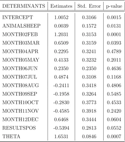
4.2.7 Logistic regression model . . . 61
4.3 Analysis of Dictyocaulus filaria egg counts . . . 63
5 Simulation Study 68 5.1 Gibbs sampler . . . 69
5.2 Simulation example . . . 70
5.3 Evaluation of predictive performance . . . 71
6 Zero Inflated Time Series Counts 74 6.1 Observation-driven models . . . 74
6.1.1 ZIP Autoregression (ZIP-AR) . . . 75
6.1.2 ZINB Autoregression (ZINB-AR) . . . 76
6.2 Illustrative examples . . . 78
6.2.1 Application to Haemonchus contortus egg counts . . . 78
6.2.2 Application to Fasciola hepatica egg counts . . . 83
7 Discussion and conclusion 85 7.1 Discussion . . . 85
7.1.1 Quantifying aggregation and zero inflation . . . 85
7.1.2 Characterise distributions applicable to count data and assess-ing their performance under zero-inflation . . . 85
7.1.3 Assessing the nature of seasonality . . . 87
7.1.4 Significance of covariates in explaining FEC . . . 90
7.2 Conclusion . . . 90
A Moment Generating Function (MGF) of the Negative Binomial
Dis-tribution 92
B R Codes 94
List of Abbreviations
AIC Akaike Information Criterion ACF Autocorrelation Function
AR Autoregressive
FEC Faecal Egg counts
GLM Generalised Linear Models HSD Honest Significant Di↵erence MCMC Markov Chain Monte Carlo MLE Maximum Likelihood Estimate
NB Negative binomial
NBD Negative binomial distribution OD VAL Optical Density Value
OLS Ordinary Least Squares PCV Packed Cell Volume PMF Probability Mass Function
QP Quasi-Poisson
ZANB Zero Altered Negative Binomial ZINB Zero Inflated Negative Binomial
ZINB-AR Zero Inflated Negative Binomial Autoregression ZAP Zero Altered Poisson
ZIP Zero Inflated Poisson
List of Figures
1 Composition of rural and commercial livestock in South Africa (Source:
Department of Agriculture, Forestry and Fisheries, 2015) . . . 3
2 Parasite species frequency distribution . . . 38
3 Coccidia eimeria and Ostertagia pinnata boxplots . . . 39
4 Boxplots of all parasite species . . . 39
5 Observed and fitted values forC. isospora . . . 46
6 Poisson residual plot . . . 46
7 Negative binomial residual plot . . . 52
8 ZIP model residual plot . . . 56
9 Cooperia isospora rootogram (Poisson and NB model) . . . 59
10 Cooperia isospora rootogram (ZIP and ZINB model) . . . 60
11 Predicted probabilities of testing negative for an infection . . . 62
12 Haemonchus contortus time series plot (time in months) . . . 78
13 ACF and Partial ACF of H. contortus . . . 79
14 H. contortus observed and fitted egg counts . . . 81
15 Fasciola hepatica time series plot (time in months) . . . 83
List of Tables
1 Parasite species names and type . . . 4
2 Summary of the reviewed literature . . . 15
3 Variable description . . . 33
4 Parasite species index of discrepancy and variance to mean ratio . . . 36
5 Kruskal-Wallis Test . . . 40
6 Poisson model selection . . . 43
7 Poisson model parameter estimates . . . 44
8 Overdispersion test . . . 47
9 Negative binomial model selection . . . 49
10 Negative binomial model parameter estimates . . . 50
11 ZIP model selection . . . 53
12 ZIP model parameter estimates . . . 54
13 ZINB model selection . . . 57
14 ZINB model parameter estimates . . . 57
15 Logistic regression parameter estimates . . . 61
16 Predicted percentage of zeroes . . . 64
17 Poisson and negative binomial parameter estimates . . . 65
18 ZIP and ZINB model parameter estimates . . . 66
19 Mean and Variance changes as sample size (N) increase . . . 69
20 Simulation results with MSE of parameters . . . 71
21 Pearson’s correlation (⇢p) and pseudo R2 . . . 72
22 Observation-drive time series models for overdispersion and zero inflation 77 23 ZINB autoregression parameter estimates . . . 80
24 Frequency distribution of observed and expectedH. contortus egg counts 81 25 5-step forecasting measures of accuracy . . . 82
26 ZIP-AR parameter estimates . . . 84
27 Parasite species AIC and AIC weights . . . 86
28 Model comparison for 15 parasite species: AIC . . . 89
Abstract
The term aggregation refers to overdispersion and both are used interchangeably in this thesis. In addressing the problem of prevalence of infectious parasite species faced by most rural livestock farmers, we model the distribution of faecal egg counts of 15 parasite species (13 internal parasites and 2 ticks) common in sheep and goats. Aggregation and excess zeroes is addressed through the use of generalised linear models. The abundance of each species was modelled using six di↵erent distribu-tions: the Poisson, negative binomial (NB), zero-inflated Poisson (ZIP), zero-inflated negative binomial (ZINB), zero-altered Poisson (ZAP) and zero-altered negative bi-nomial (ZANB) and their fit was later compared. Excess zero models (ZIP, ZINB, ZAP and ZANB) were found to be a better fit compared to standard count models (Poisson and negative binomial) in all 15 cases. We further investigated how dis-tributional assumption a↵ects aggregation and zero inflation. Aggregation and zero inflation (measured by the dispersion parameterk and the zero inflation probability
⇡) were found to vary greatly with distributional assumption; this in turn changed the fixed-e↵ects structure. Serial autocorrelation between adjacent observations was later taken into account by fitting observation driven time series models to the data. Simultaneously taking into account autocorrelation, overdispersion and zero inflation proved to be successful as zero inflated autoregressive models performed better than zero inflated models in most cases.
Apart from contribution to the knowledge of science, predictability of parasite bur-den will help farmers with e↵ective disease management interventions. Researchers confronted with the task of analysing count data with excess zeroes can use the find-ings of this illustrative study as a guideline irrespective of their research discipline. Statistical methods from model selection, quantifying of zero inflation through to accounting for serial autocorrelation are described and illustrated.
Keywords: Aggregations, autoregressive models, Akaike information criterion, cor-relation, count data, exponential family, generalised linear models, goats, internal parasites, hosts, negative binomial distribution, overdispersion, Poisson distribution, sheep, time series and zero inflation.
1
Introduction
In this section the following are outlined: background, justification, and purpose of the study together with the problem statement. The nature of the data is highlighted together with some inherent issues. We then propose statistical models that solve the problem of overdispersion, zero inflation and serial correlation in count data. Out-lining research objectives and noting that the study is solely for illustrative purpose conclude this chapter.
1.1
Background
One of the major challenges faced by the agricultural sector today is that of food security. Food security not only relates to the availability and a↵ordability of ba-sic food products but also relates to the self-sufficiency of a nation in producing food and fibre products (McLeod et al., 2008). Both livestock products and produce (field crops and horticulture) contribute to food security. In relation to produce, livestock products make up 47% of the gross agricultural product (Meissner, et al., 2013). According to the abstract of agricultural statistics (Department of Agricul-ture, Forestry and Fisheries, 2015) there are 24.6 million sheep and 7.0 million goats in South Africa, both in rural and commercial farms. Of the total, 3.1 million sheep and 4.9 million goats are reared by rural farmers and not commercially (see Figure 1). Challenges these rural farmers face include among others, access to market and e↵ective disease management. Diseases in livestock can be both bacterial, viral and also parasitic diseases. In this study the focus is on guiding parasites diseases control measures through understanding of how parasites are distributed among their hosts. South African rural communities primarily practice subsistence farming. Livestock production as a result is directly linked to the wellbeing of the communities. Out-break of an infectious livestock disease thus threatens not only the production but also the wellbeing of the farming community. Parasitology studies are characterised by count data, involving presence and absence of faecal eggs of di↵erent species, which occur at di↵erent time of the year.
Understanding the nature of the distribution of such data and the frequency of occurrence of the species would guide in timely introduction of control interventions. Faecal egg count are generally performed on livestock to monitor the level of par-asitism in the herd, determine the e↵ectiveness of certain treatments or determine which animals are resistant to parasite species of interest. In the area of quantitative
parasitology, counts data are commonly used to understand the interaction between parasites and their host. Crofton (1971) suggested the use of a frequency distribu-tion, both in expressing a quantitative relationship between parasites and their hosts and in understanding prevalence and abundance patterns.
Figure 1: Composition of rural and commercial livestock in South Africa (Source: Department of Agriculture, Forestry and Fisheries, 2015)
While prevalence is the propor-tion of infected hosts among all hosts examined, abundance is the number of parasites found on all hosts. Both prevalence and mean abundance are impor-tant measures in indicating the level of parasitism in the herd. They give information on the skewness of the distribution and the proportion of zero counts. Most parasites are aggregated among their hosts, rendering traditional statistical methods ine↵ective. O’Hara and Kotze (2010) cautioned against the use of log transformation on count data, suggesting the use of standard count models i.e. Generalised Linear Models (GLMs). The motivation behind this study is its multidisciplinary nature and the opportunity it presents in pulling together distributional theories and applying them to livestock faecal egg count (FEC) data. Understanding the distribution of these FEC will help in iden-tifying when the host are most susceptible and thus the most appropriate time for remedial measures to ensure maximum herd productivity.
1.2
Data Description
The data in this study is observational and was collected from January 1998 to Febru-ary 1999 in three di↵erent open grazing regions in the Free State province; Kenstell, QwaQwa and Harrismith. Feaces (dung) from identified animals were examined for parasite species eggs, each animal’s dung was examined once. Upon examination, parasite species were identified and the following were recorded: the time of data
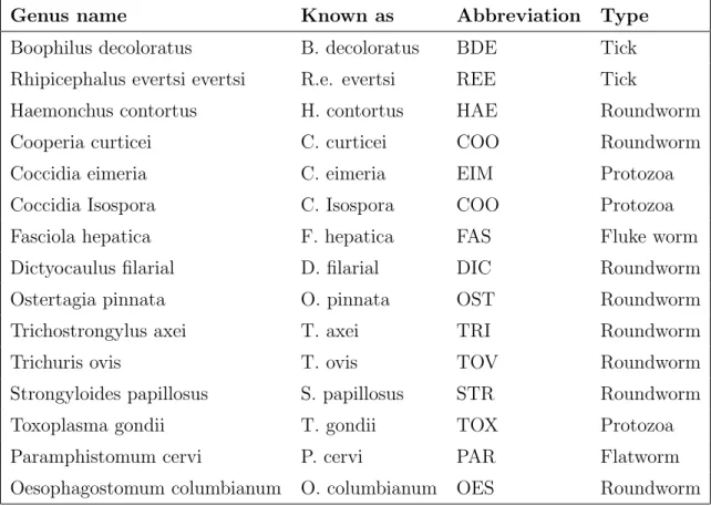
collection in months, the age, type (whether it was a sheep or goat) and sex of the ruminant. Blood test were also performed and packed cell volume and infection test results were also recorded, optical density and inhibition percentage were then deter-mined. A total of fifteen di↵erent parasite species were identified while 495 animals (sheep and goats) were examined. We use the data on a secondary level and for illustrative purposes, the data was originally collected by Mogaswane K.H.R., Mtsali M.S. and Tsotetsi A. from the University of the North, Qwaqwa campus.Table 1 shows the name and type of parasite species that were identified.
Table 1: Parasite species names and type
Genus name Known as Abbreviation Type
Boophilus decoloratus B. decoloratus BDE Tick
Rhipicephalus evertsi evertsi R.e. evertsi REE Tick
Haemonchus contortus H. contortus HAE Roundworm
Cooperia curticei C. curticei COO Roundworm
Coccidia eimeria C. eimeria EIM Protozoa
Coccidia Isospora C. Isospora COO Protozoa
Fasciola hepatica F. hepatica FAS Fluke worm
Dictyocaulus filarial D. filarial DIC Roundworm
Ostertagia pinnata O. pinnata OST Roundworm
Trichostrongylus axei T. axei TRI Roundworm
Trichuris ovis T. ovis TOV Roundworm
Strongyloides papillosus S. papillosus STR Roundworm
Toxoplasma gondii T. gondii TOX Protozoa
Paramphistomum cervi P. cervi PAR Flatworm
Oesophagostomum columbianum O. columbianum OES Roundworm
The observed sheep and goat‘s faecal egg count shows that for 14 of the 15 para-site species has more than 50% of zero counts. Parapara-site counts tends to be overly dispersed (especially if the datasets are zero abundant) with a few hosts harbouring most of the parasite while the majority of the population has low counts. This poses problems in both descriptive and inferential statistics. In descriptive statistics, there
is a question of whether the mean is the best measure of location when the underlying distribution is aggregated. The sample mean tends to be overly influenced by large values in heavily skewed distribution while the geometric mean cannot be determined directly if the data set has zero values.
In inference, most readily used statistical procedures i.e. ordinary least square method in regression analysis, assumes normality of the error terms. When the dis-tribution of faecal egg counts tends to be aggregated among their hosts, alternative methods for analysing the data are considered.
1.3
Justification
Count data with numerous zeroes is often heavily skewed and hardly conform to nor-mality assumptions and conventional transformation approach does not resolve the problem. A general linear model addresses this concern. Count data mostly does not follow a normal distribution; log transformation becomes questionable in the event that the data is abundant with zeroes. A conventional technique such as ordinary least squares (OLS) in linear regression results in multiple assumptions being vio-lated. Developed with the aim to address the limiting assumption of normality in linear models, the general linear model is an extension of linear models that allows one to specify the distribution of data via a link function. If parasite encounters with hosts are completely random then the faecal egg count per host are expected to follow a Poisson distribution. The overly dispersed nature of parasitology data again creates a problem in this regard as the variance is usually greater than the mean while a Poisson process has a variance equal to its mean. Given its nature to deal with the issue of over dispersion as compared to the Poisson distribution, the negative binomial distribution (NBD) has historically been widely used in modelling, quantifying or analysing parasite distribution (Gaba, et al., 2005). Distributions that are less restrictive on assumptions in handling of the count data in the presence of many zeroes are considered.
The aim is to package together the di↵erent distributions that are considered in quantifying parasite distribution in count data and also count data in other areas in general. Developing models which provide efficient estimates on abundance of disease causing parasites will enable implementation of interventions on the health life of livestock feasible and the livelihood of rural community will subsequently be improved.
The findings will provide a step by step quantitative guideline to researchers in areas of ecology and parasitology interested in modelling occupancy abundance or prevalence patterns. Researchers will be able to apply the simplest count data model (the Poisson distribution) and also move to more complex models that explain aggre-gation in count data. Problems arising from model misspecification such as inflated standard errors will be made aware to researchers. In a nutshell, results from this study will help researchers dealing with count data to apply a spectrum of models that could be applicable in their studies and provide them with a tool to choose the best model given their particular case.
1.4
Purpose
Livestock keeping in South Africa plays a major role in the livelihood of rural com-munities. Some of these roles include; livestock keeping as a source of income and cultural activities that relates to both the wellbeing of the community and house-hold. Other secondary roles include livestock keeping to create employment and for companionship purposes. Community grazing adapted by rural society provides ideal ground for parasitological diseases to flourish. Developing control systems through use of good statistical models will lead to timely implementation of the control inter-ventions. This study tends to quantify patterns of di↵erent parasite species among their hosts and to investigate any changes in these patterns across time, host gen-der, host age and the type of livestock in question. Upon completion of this study researchers interested in quantifying count data, either for productivity or cost re-duction reasons will use the findings. The researchers will be guided in choosing the best distribution applicable to their count data and steps in conducting the analysis.
1.5
Problem statement
Livestock keeping in a communal grazing setup in certain parts of South Africa is characterised by animal diseases caused by parasitological species. The produce from these livestock is minimal while the mortality is high. Understanding the distribu-tion of disease causing species through analysis of faecal count data characterised by zeroes, guide in formulation of e↵ective interventions.
To understand the distribution of these infectious species, first we focus on the nature of the faecal count data. Some characteristics of the faecal count data require special attention before any analysis methods is identified. Exploring of the data indicated that a majority of the hosts (animal species) recorded low or zero egg counts while
a few recorded very high counts. This results in a phenomenon known as parasite aggregation among hosts. The presence of aggregation creates a problem in terms of applying the simplest count data model, which is the Poisson count model. Extra variation around the mean more than expected by the Poisson model requires a more flexible distribution such as the negative binomial distribution. Another considera-tion with the FEC data is the presence of too many zero counts. A way to deal with excessive zeroes is to employ zero inflated models which better account for the extra variation caused by the excess zeroes.
Data are available on 15 parasite species and the challenge in this study is inves-tigating which distribution explains each parasite species and if indeed all the par-asite species are aggregated among their host population. The procedure involves fitting some discrete probability distributions applicable for count data, namely; the Poisson, quasi-Poisson, Negative Binomial (NB), zero inflated Poisson (ZIP), zero altered Poisson (ZAP) and zero inflated negative binomial (ZINB) and zero altered negative binomial (ZANB) distribution (also called Hurdle Models). The last four address the problem of excessive zeroes.
1.6
Research objectives
Keeping in mind that the aim is to illustrate how to handle three main distinctive features (autocorrelation, overdispersion and zero inflation) of count data. The main objective is to review the existing distributions that fit aggregated count data and de-termine the appropriate model for parasitological data characterised by many zeroes. The following are the specific objectives:
• Quantify aggregation and zero inflation models. • Characterise distributions applicable to count data.
• Assess the performance of these distributions in the presence of numerous ze-roes.
• Determine the significance of covariates in explaining variation in the observed faecal egg counts.
• Check the consistency of the fitted models by simulating random observations from zero inflated distribution.
2
Literature Review
In this section a thorough review of literature is conducted. The review first looks at application of standard count models in both areas of ecology and parasitology. We then focus on studies that address both issues of zero inflation overdispersion and how they compare with standard Poisson and NB distributions. A summary of the literature review is provided at the end of this chapter.
2.1
General approach to modelling count data
The simple and most common initial approach to count data is assuming a Poisson counting process. The Poisson distribution assumes that counts per unit time or space are randomly distributed with the mean equal to the variance. While the Pois-son distribution is favoured because of its simplicity, the downside is that it does not take into account overdispersion. This in turn leads to overestimation of standard er-rors, resulting in significant covariates that would have otherwise not been significant. A more flexible approach to count data is to use a negative binomial distribution. A negative binomial distribution assumes various quadratic mean-variance relation-ship. Di↵erent parameterisations of the negative binomial distribution results in the Negative Binomial1 (NB1), Negative Binomial2 (NB2) and Negative Binomial12 (NB12) models (later explained in section 2.3). The advantage of a negative bino-mial distribution over the Poisson distribution is ability to account for overdispersion. However, in the presence of excess zeroes the negative binomial distribution may not sufficiently explain the distribution of parasites among hosts. Inability of standard count models to account for zero inflation leads to the need to apply count models for excess zeroes. Generalised Linear Models (GLMs) that account only for zero in-flation do not take into account possible correlation between latent variables. Yang, et al., (2015) proposed the use of parameter driven state-space time series models to account for temporal correlation. Zero inflated time series count models will not only account for overdispersion and zero inflation but also for possible correlation between observations (Maiti, et al., 2014).
2.2
Lognormal distribution and logistic regression
Using logistic regression and lognormal distribution, Baines, et al., (2015) found the factors; month, year, sex, age and group size to be significant in explaining the occur-rence and seasonality of internal parasites elephants. For cases where prevalence was 100%, logistic regression was inappropriate, as counts cannot be reduced to binary
response but a single response. Instead a log transformation was done on counts and a linear regression was used to investigate the occurrence of parasite species. Sileshi (2008) applied logarithmic transformation to stabilise the variance and normalise the counts by taking the log (count+ 1), a lognormal distribution was then used to explain the soil organism’s abundance patterns. Normality tests on the transformed counts indicated that, the transformation did not achieve the desired results on most of the data sets. The data were still not normally distributed upon transformation. Even though Sileshi (2008) and Baines, et al., (2015) performed log transformation on counts, we decided not to transform the parasite species egg counts. This is because transformations (either log transformation or square root transformation) always performed poorly compared the Poisson distribution (O’Hara, et al., 2010). O’Hara, et al., (2010) conducted a simulation to compare the performance of the negative binomial distribution (NBD) to that of the lognormal distribution. They found that NB model consistently performed well and e↵ectiveness of transformation decreased with an increase in the number of zeroes. For this reason the lognormal distribution is not included in our study. However, a normality test on the trans-formed data is included (in the preliminary data exploration section) to support the exclusion of a lognormal distribution.
Apart from count models, Ziadinov, et al., (2010) added logistic regression to their analysis to model prevalence of infections. Prevalence of infection is the proportion of infected host among all host examined. The use of logistic regression is instinctive and largely depends on the aim of individual studies. Logistic regression condenses count data into binary data which potential hides crucial information in the data. With regard to predicting the prevalence pattern (i.e. the percentage of zeroes), logistic regression outperformed count models (Lewin, et al., 2010). While Bailey, Lopez, Camero, Taiquiri, Arhuay and Moore (2013) used logistic regression to in-vestigate the risk factors associated with prevalence of parasitic infection in street children, Ajiferuke and Famoye (2015) used lognormal regression in modelling simu-lated counts response. Compared to lognormal and Poisson regression, the negative binomial regression was found to be a better fit mostly due to the overdispersed counts.
2.3
Common models for count data
The two most widely applied distributions in count data are the Poisson distribution (applicable when internal parasites are randomly distributed among their hosts) and the NB distribution (applicable in the event of overdispersion). When modelling rare
species (parasite a↵ecting a smaller proportion of the herd or organism that are scat-tered in their environment), researchers historically applied standard count models. The problem with rare species data is the higher proportion of zeroes than expected by the standard count models. Lambert (1992) introduced the use of zero inflated models to handle the problem of excessive zeroes in count data. Ziadinov, et al., (2010) however concluded that excessive zeroes in count data does not necessarily imply the application of zero inflated models. Historically, the negative binomial dis-tribution has been widely used to both quantify aggregation and analyse count data. This has mainly been due to its simplicity, the ability to deal with overdispersion and the availability of software. In this review the focus is on methods and proce-dures used in analysing the data and research findings as relevant to the objectives of our study. Papers on count data with overdispersion are reviewed together with count data with excessive zeroes. Objectives for count data with overdispersion were primarily centred on comparing the fit of the negative binomial distribution to other distributions with focus on estimating the e↵ects of covariates.
Two of the research objectives are characterising distributions applicable to counts data and quantifying aggregation. Distributions applicable to count data accord-ing to Gaba, et al., (2005) include the NBD, log-normal, exponential and Weibull distribution. In addition to fitting the negative binomial model both Linden and Mantyniemi (2011) and Ver Hoef and Boveng (2007) added the Poisson model with a linear mean-variance relationship (Quasi-Poisson) in analysing count data distri-butions. A common tread throughout the study by Gaba, et al., (2005), Linden and Mantyniemi (2011) and Ver Hoef et al., (2005) is the use of maximum likelihood in parameter estimation and a choice of the negative binomial model as an initial approach in analysing count data. To quantify aggregation, Gaba et al., (2005) and Linden et al., (2011) applied the variance to mean ratio as an aggregation measure. The variance to mean ratio as the name suggests is calculated as the ratio between the variance and the mean. Aggregation occurs when there is more variation around the mean than expected by the Poisson distribution. A value greater than one for the variance-mean ratio is indicative of aggregation while values less than one indicate the absence thereof. Other measures of aggregation available in literature include the index of discrepancy but in most studies only the variance to mean ratio is used, e.g. Marques, et al., (2010) and Alexander (2012) used only the variance to mean ratio as aggregation measure of parasite counts.
While the focus with Gaba, et al., (2005) was to compare the NBD with other distribution, Linden and Mantyniemi (2011) compared only di↵erent
parameterisa-tion of the NBD with a wide range of mean-variance relaparameterisa-tionships. Derivaparameterisa-tion of the formula below shows how the negative binomial distribution is formulated with di↵erent variance to mean relationships. Let
2 =!µ+✓µ2,
where 2and µare the variance and mean of the NB distribution, respectively. Both
!and ✓ are termed overdispersion parameters, with their di↵erent values giving rise to di↵erent parameterisation of the negative binomial distribution. We assume the probability mass function (PMF) of the NB distribution takes form:
P(Y =y) = ✓ y+r 1 y ◆ pr(1 p)y y = 0,1,2, . . .
Using the moment generating function of the negative binomial distribution (NBD) in appendix 1, we derived the quadratic mean variance relationship of the NBD. From appendix 1; µ= r(1 p) p , and 2 = r(1 p) p2 .
From theµ expression:
µp = r rp p(µ+r) = r
p = r
µ+r.
It then follows that:
1 p = 1 r µ+r = µ+r r µ+r = µ µ+r.
Substituting (1 p) into the expression for 2 we obtain: 2 = r(1 p) p2 = r⇣µ+µr⌘ ⇣ r µ+r ⌘2 = µr µ+r (µ+r)2 r2 = µ(µ+r) r = µ 2 r +µ.
Replacing the aggregation parameter 1r with the aggregation parameter✓and letting
!= 1 we obtain:
2 =!µ+✓µ2.
Fixing the value of ✓ at zero results in a linear variance mean relationship (Quasi-Poisson model also termed NB1). The value of!can also be fixed at one, resulting in a quadratic mean variance relationship (NB2). Another form of a negative binomial distribution (NB12) is obtained by not fixing either ! or ✓ but letting them take specified constant values. Apart from performing a comparative study, Linden and Mantyniemi (2011) also wanted to highlight the relationship between the standard count model (Poisson model) and the variations thereof at di↵erent overdispersion level. To decide on the choice of the model, environmental factors such as flocking patterns of the birds were used in conjunction with statistical measures such as the AIC.
The Akaike‘s Information Criterion (AIC) was used to select the best model that had the minimum AIC. Gaba, et al., (2005) took a further step by calculating AIC weights (wi), the probability that a model is the best one among the set of candidate models for the observed data. Let;
wi=
e 0.5 i
PR
j=1e 0.5 j
whereR is the number of models in a set and being the AIC di↵erence, calculated as AICi AICmin, where AICmin = min[AIC1, ..., AICR]. AIC di↵erence can also be used to determine the level of practical support to a model given the best model. Using these AIC di↵erences, Gaba, et al., (2005) found the Weibull distribution to provide a better fit to most of the dataset followed by the NBD. The choice of the best model was not solely based on the AIC but also on a simulation study to determine the bias and consistency of estimators.
2.4
Models for excess zeroes in count data
Zero inflated models are introduced. In this section we propose to apply zero inflated models to test for zero inflation both in the presence and absence of overdispersion. In addition to characterising distributions applicable to count data, another objec-tive is to quantify both aggregation and zero inflation. Vidyashankar, et al., (2012) suggested the use of zero inflated Poisson and zero inflated negative binomial distri-bution in modelling the resistance (pre and post treatment distridistri-butions) of equine gastrointestinal nematodes to treatment. Lewin, et al., (2010) studied fish catch data collected at di↵erent geographical sites, a large number of zero catches were observed. In addition to the standard count models, zero inflated, zero altered and logistic re-gression models were added to the analysis. The adequacy of each distribution was tested using the ratio or the deviance and the degrees of freedom (D/DF). Sileshi (2008) first checked the adequacy of standard count models using the ratio (D/DF) in his study on soil animal counts. Ratios greater than one indicate some degree of overdispersion unaccounted for and inadequacy to use the model under concern, whereas ratios around one indicate the appropriateness to apply the model. Both Sileshi (2008) and Vidyashankar, et al., (2012) found the Poisson distribution inade-quate with large values of the ratio of deviance and degrees of freedom. Vuong tests (Vuong 1989, cited in Lewin, et al., 2010) were used to compare non-nested models. Vuong test is a likelihood-ratio-based test for model selection based on closeness of model to the true data. The models can be nested or non-nested.
Vuong test favoured models that accounted for excess zeroes each time two models (standard count model and count models for excess zeroes) were compared (Vuong 1987, cited in Lewin., et al, 2010). The null hypothesis that standard count models and count models for excess zeroes are equally close to the observed counts was re-jected in all cases, favouring models that account for excess zeroes. To check overall statistical significance of covariates, Lewin, et al., (2010) compared the final
regres-sion models to the null models with only the intercept. All count models with full sets of covariates were better in explaining abundance pattern, however there was low improvement in McFadden R2 value. McFadden R2 is a pseudo coefficient of determination that is similar to the r2 in ordinary least squares (OLS) regression, the low improvement in this value from the full to the null model is an indication that some factors that a↵ect the abundance pattern might not have been recorded Lewin, et al., (2010).
2.5
Summary of the reviewed literature
Table 2 provides the summary of the literature review covered. It should be noted that only the purpose and conclusions relevant to this current study have been in-cluded in the review summary table. From the review, apart from Lewin et al., (2010), authors either compared two distributions, only used standard count models or zero inflated models in modelling prevalence patterns. In this study we continue with sets of distribution applied by Lewin., et al., (2010) but apply it in areas of parasitology instead of ecology. We use this range of count data models to provide guideline to researchers in characterising aggregation and modelling prevalence and abundance.
Ta b le 2: S u m m ar y of th e re v ie w ed li te ra tu re C it a ti o n C o un ts A re a P ur p o se C o ncl us io n Aj if er u ke , et al ., (2015) S im u la ted cou n ts S ta ti st ics S im u la ti on st u d y O ver d isp er sed co u n ts w er e b et ter m o d el led b y th e n eg -ativ e binomial distribution. Bai n es, et al ., (2015) In ter n al p ar a-si tes P ar as it ol og y M o d el lin g o cc u rr en ce an d season al it y of in ter n al p ar -asites in wild elephan ts. Ag e, gr ou p si ze , se x m on th and year w ere found to b e si gn ifi can t co var iat es. Y an g, et al ., (2015) W or k p la ce in -ju ri es Bi ostati sti cs Dev el op in g m o d el li n g fr am ew or k to accom m o d at e thre e fe ature s; ov erdis p er-si on , zer o in fl ati on an d auto correlation Dynamic ze ro inflate d P ois -son m o d el w as fou n d to b e ad eq u at e in m o de ll in g al l thre e fe ature s. Mai ti , et al ., (2014) S im u la ted cou n ts S ta ti st ic s C omp ar in g st at io n ar it y and auto correlation structures. In th e p resen ce of ex cess ze ro es , ze ro infl at ed P oi s-son au to-r egr essi ve p ro cess of order 1 p erformed b etter. Vi d ya sh an ka r, et al ., (2012) Gast roi n test in al n em at o d es V et er in ar y P ar a-si tol ogy In vest iga ti n g an th el m in ti c re si st an ce to co n tr ol eq u ine gastroin testinal nemato des. Both p re an d p ost treat-m en t d ist ri b u ti on w er e fou n d to b e zer o in fl at ed (w ith the ze ro inflate d Po is so n p rov id in g a b et te r fit). Linde n, et al., (2011) Bi rd s Mi grati o Ecol ogy Mo d el p rev al en ce u si n g d if-fe re n t p ar ame tr is at io n of th e NB D . NB D p ro v id e b et te r fi t co m -p ar ed to P oi sso n d ist ri b u -tion. V au d or , et al ., (2011) F re sh w at er fi sh E co lo gy C om p ar at iv e st u d y. NB D p ro v id ed a b et te r fi t to 58% of the datas ets com-p ar ed to zer o in fl at ed m o d -el s. Le w in, et al., (2010) Fi sh C at ch E co lo gy M o d el li n g co u n ts w it h ex -cess zer o es. Hu rd le m o d el s an d ze ro in fl at ed m o d el s p er fo rm ed b et ter th an st an d ar d co u n t m o d el s. Continue d on next page
Ta b le 2 – Continue d fr om pr evious page C it a ti o n C o un ts A re a P ur p o se C o ncl us io n O ’Ha ra , et al ., (2010) S im u la ted Cou n ts S ta ti st ic s C omp ar at iv e st ud y. L og tr an sf or m ed co u n ts p ro v id es w or st fi t co m p ar ed to coun t mo de ls . Zi ad in ov, et al ., (2010) F ox es In ter n al Pa ra si te s V et er in ar y P ar a-si tol ogy Mo d el li n g p rev al en ce p at -te rns . Zero in fl ated m o d el s can b e d isp en sa b le in m o d el li n g cou n t d at a wi th ex cess ze-ro es . S il esh i (2 00 8) Ex ter n al P ar a-si tes Pa ra si to lo gy C om p ar at iv e st u d y : M o d -el li n g co u n ts wi th ex cess ze-ro es . De spite a high prop ortion of ze ro es in th e d at a, NB D w as ab et te rfi tt o 75 %o ft h e d at aset s co m p ar ed to ex cess zer o m o d el s. V er Ho ef , et al ., (2007) Ha rb ou r S ea l E co lo gy C om p ar at iv e st u d y. D i ↵ er -en t m ea n -v ar ia n ce re la ti on-sh ip s. Com p ar at iv e st u d y. Qu assi -Po is so n p rov id ed b et te r fi t th an NB D . Gab a, et al ., (2005) S h eep Macr op ar asi tes P ar as it ol og y C h ar ac te ri se Ag gr eg at io n V ar ia n ce to m ea n ra ti o, ag -gregation parameter of the NB d is tr ib u ti on and sc al e p ar am et er of th e W ei b u ll d ist ri b u ti on u sed to ch ar ac-te ris e aggre gation. S h aw, et al ., (1998) Wi ld li fe Macr op ar asi tes Pa ra si to lo gy C om p ar e p er fo rm an ce of NB D w it h P oi ss on d is tr ib u -tion. NB D b et te r d es cr ib es ag -gregated coun ts that P ois-son d ist ri b u ti on . L am b er t (1 99 2) D ef ec ts M an u fa ct u ri n g Ap p ly a Z IP m o d el to cou n ts of d efect ed wi ri n g b oa rd s. Z IP p re d ic te d d ef ec ts b et te r than standard coun t mo d-el s. Cr oft on (1971) F resh W at er Or -ganisms E co lo gy C om p ar at iv e st u d y. NB D tr u n ca te d at va ri ou s va lu es p ro v id es a b et te r fi t. Cr oft on (1971) F resh W at er Or -ganisms E co lo gy C om p ar at iv e st u d y. NB D tr u n ca te d at va ri ou s va lu es p ro v id es a b et te r fi t.
3
Statistical Models on Count Data
Consider count data as data in which observations take only nonnegative integers and where these integers arise from counting rather than ranking. Conventional approaches in data analyses consider linear regression, which not only assumes nor-mality but also heterogeneity and independence. Even though a normal distribution is continuous, the Gaussian linear regression model is still applicable in analysis of count data; however it is not the best option (Zuur, Leno, Walker, Savelier and Smith, 2007). With some data transformation the lognormal distribution is also an applicable fit to count data. A new response variable (Ynew), is usually calculated as the original observed count plus one and natural log transformation [Ln(Ynew)] is assumed to be normally distributed. Gaba et al., (2005) fitted the normal distribu-tion and the lognormal distribudistribu-tion to counts of nematodes macroparasites found on sheep. The normal and the lognormal distributions more often provided the worst fits compared to other distributions. O’Hara et al., (2010) cautions against log trans-formation of count data and argues that generalised linear models (GLMs) are better suited in dealing with count data, especially in the presence of overdispersion. Gen-eralised linear models are an extension of linear models which allows the response variable to follow any member of the exponential family of distributions. In our case two of the distributions of interest are members of the exponential family (Poisson and Negative binomial). GLMs consist of three components;
1. The random component which specifies the conditional distribution of the re-sponse variable given a set of explanatory variables,Yi|Xi, whereY is the data vector andX is the design matrix.
2. The systematic component which specifies the linear function of the explana-tory variables (also called the linear predictor) on which the expected value of the response variable, µi depends on.
⌘i= ↵+ 1Xi1+ 2Xi2+. . .+ kXik, where↵ and 1, ..., k are unknown regression coefficients.
3. The link function which describes how the expected value of the response vari-able, µi is linked to a set of covariates through a linear predictor. A log link function is usually used for counts as it ensures predicted outcomes do not go below zero.
The mean can thus be estimated as:
µi =e↵+ 1Xi1+ 2Xi2+...+ kXik.
3.1
The exponential family
According to Cox and Hinkley (1979), any discrete or continuous random variable
Yi that takes on the general form below is classified as a member of the exponential family.
f(yi,✓i, ) =exp ⇢
yi✓i b(✓i)
a( ) +c(yi, ) , i= 0,1,2, ..., n,
where is the scale parameter,✓is the link parameter anda(.), b(.), c(.) are functions which determine the distribution when specified and n is the number of observations. The mean and the variance are given by:
E(Y) =b0(✓)
V ar(Y) = b00(✓).
The Poisson and the NBD are thus members of the exponential family. Even though the probability mass function (PMF) of the zero-inflated and zero-altered distribu-tions cannot be expressed as exponential family, GLM theory can still be used in applying these distributions. As a result zero inflated distributions will be applied in explaining the distribution of the parasite counts.
3.2
The Poisson distribution
We first start by showing that the Poison distribution is an exponential family mem-ber with the mean and the variance of . SupposeY ⇠P oisson( ). From appendix A the probability mass function (PMF) of Y is:
P(Y =y) = e y y! y = 0,1,2, ... = exp log ✓ e y y! ◆
= exp[loge + log y logy!] = exp[ +ylog logy!].
Comparing the expression with the general exponential family form it is clear that the Poisson distribution is a member of the exponential family with:
✓ = log
b(✓) =
a( ) = 1
c(y, ) = logy!.
From the expression above we can write:
e✓ = elog
= .
For any member of an exponential family we know thatE(Y) =b0(✓) andV ar(Y) =
b00(✓).
)E(Y) =e✓ = and
V ar(Y) =e✓ = .
We can see that the mean and the variance of a Poisson distribution are equal and that the canonical link linking E(Y) and the parameter ✓ is a log link, that is
g(µ) = log =✓.
Maximum likelihood estimation
Taking the logarithm of the likelihood function makes it additive. Unknown pa-rameters can then be estimated taking the first-order derivative of the log likeli-hood function with respect to unknown regression parameters and setting it to zero. Second-order derivatives of the log likelihood function are used in calculating the standard errors of estimates. Unlike linear regression analysis which results in closed form solution for parameter estimates, the Poisson GLM (along with other distribu-tions) results in equation that must be solved iteratively. Using iterative reweighted
least squares such as Fisher scoring or Newton-Raphson unknown parameters can be estimated. Substituting the estimated regression parameters in the mean expression an estimate for µi can be obtained. For any given µi the probability of observing a count yi can be estimated. The log-likelihood (l);
l = log(L) = n X i=1 [yilog(µi) µi log(yi!)] = n X i=1 [yi(x 0 i ) e x0i i log(yi!)].
The partial derivative with respect to :
l = n X i=1 xiyi xiex 0 i = n X i=1 xi(yi ex 0 i ) = n X i=1 xi(yi µi).
The estimating equation can then be written as a function of and is solved itera-tively using Newton-Raphson method.
n X
i=1
xi[yi µi( )] = 0.
We use the Newton-Raphson method that proceeds iteratively to estimate the pa-rameters, according to Hardin and Hilbe (2012) if (t) is the starting point and t takes on any integer, the next value is obtained as:
(t+1)= (t) Ht 1g(t),
g(t) is the log-likelihood first partial derivative, evaluated at (t). H(t) is the second partial derivative, also called Hessian (evaluated at (t)).
For the Poisson model:
g = n X
i=1
and H = n X i=1 ˆ µixix 0 i. . 3.2.1 Goodness of fit
The deviance is defined as twice the di↵erence between the log likelihood of the model that provides the best fit from the model under study (Zuur, et al., 2007). In generalised linear model theory, the deviance is similar to residual sum of squares in linear models. A deviance decrease constitutes an improvement in model fit, if the model is an exact fit to the data deviance is zero.
D = 2[l(y;y) l(y; ˆµ)] = 2 n X i=1 [(yilog(yi/µi) (yi µi))],
whereD is the deviance andlis the log-likelihood function. A similar measure toR2 in GLM is called the explained deviance, the portion of the null deviance accounted for by the model. The null deviance is the residual deviance of the intercept only model. LettingD0 be the null deviance andD1be the residual deviance of the model in question, the explained deviance can be calculated as:
R2 ⌘1 D1
D0
.
3.2.2 Model selection
Model selection is done to ensure important explanatory variables are included in the model. For model selection, the Akaike Information Criterion (AIC) is used. If we have two models M1 and M2, where M2 is a sub-model of M1 and D1 and
D2 are their deviance respectively. The drop1 command in R performs a likelihood ratio test with the di↵erence between the deviances approximated by a Chi-Square distribution.
D2 D1⇠ 2(p q).
Where p and q are number of parameters for models M1 and M2 respectively, with
q < p. p and q are the number of parameters in model M1 and M2 respectively. The null hypothesis is that the regression parameter i (the dropped variable in the sub-model M2) is equal to zero.
3.2.3 Overdispersion
When there is evidence that the variance is greater than the mean, then there is overdispersion. In exploring our data informally, the computed variance to mean ratio and index of discrepancy indicated possible overdispersion. Hardin and Hilbe (2008) suggest a regression based test for overdispersion, where under the null hy-pothesis the variance is equal to the mean. To run the test, first the fitted values and the test statistic,Z, need to be calculated and then regress the test statistic, Z, as intercept only model. Z is standard normal distributed with the mean of 0 and the variance of 1, Z⇠(0,1). Z = (yi µˆi) 2 y i ˆ µi p 2 .
When dealing with overdispersion in a Poisson regression, a quasi-Poisson GLM can be employed. A quasi-Poisson GLM is a Poisson GLM in all aspect, except that the variance is specified as a linear function of the mean.
var(Yi) = µi.
Adding the dispersion parameter will inflate the standard errors in the e↵ort to adjust for overdispersion. This can be a downside if the model is misspecified, as parameters will become less significant. Similar to Poisson GLM, the drop1 command in R will be used for model selection. For hypothesis testing however, the new test statistic follows an F distribution (Hilbe and Hardin, 2012).
(D2 D1)/(p q)
ˆ ⇠F(p q, n p). 3.2.4 Model validation
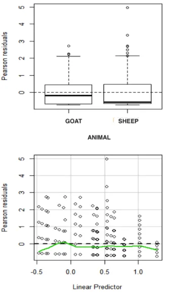
Residual analysis and plots are used in model validation. The variance of the Poisson distribution increases with larger mean values, as a result the standard residual cannot be useful. In GLMs either the Pearson’s residuals or the deviance residuals can be employed in model validation (Hilbe, 2014). The Pearson’s residuals are just the standardised residuals divided by the square root of the variance of Yi.
The standardised residuals are defined as the di↵erence between observed and fitted values,yi µˆi, for i= 1, ..., n
"pi = pyi µˆi
V ar(µi)
.
Deviance residuals on the other hand can be calculated as;
"Di =sign(yi µi) p
di,
where di is each observation’s contribution to the deviance. Both the residuals can then be plotted against the fitted values and each explanatory variable to check for any patterns in the plots. If there are any patterns in the plot necessary changes will be implemented, e.g. including some of the explanatory variables that were initially omitted. If the problem persists then a distribution that addresses overdispersion will be fitted.
3.3
The negative binomial distribution
We begin by showing the connection between the Poisson and the negative binomial distributions. To achieve this we derive the negative binomial distribution from the first principles. Suppose Yi| i follows a Poisson distribution with conditional mean E(Yi| i) = µi and the parameter, i, follows a gamma distribution with the mean E( i) =µi and variance var( i) =µ2i↵ 1.
P(Yi =yi| i) = e i yi i yi! and g( i) = ↵ 1 i e i/ (↵) ↵ , i >0. The joint density ofYi| i is then given by:
P(Yi =yi| i)g( i) = e i yi i yi! ↵ 1 i e i/ (↵) ↵ .
We now show that the marginal distribution ofYi follows a negative binomial distri-bution. P(Yi =yi) = Z 1 0 P(Yi =yi| i)g( i) d i = Z 1 0 e i yi i yi! ↵ 1 i e i/ (↵) ↵ d i = 1 (↵) ↵ Z 1 0 e i yi i yi! ↵ 1 i e i/ d i = 1 yi! (↵) ↵ Z 1 0 ↵+yi 1 i e i(1+1/ ) d i = 1 (yi+ 1) (↵) ↵ (yi+↵) ✓ + 1 ◆yi+ i = ✓ yi+↵ 1 yi ◆ ✓ 1 + 1 ◆↵✓ 1 1 + 1 ◆yi .
Looking at the expression of the negative binomial distribution in the next para-graph, we can conclude that the marginal distribution of Yi is a negative bino-mial distribution with r = ↵ and p = 1/( + 1). The E( i) = µi = ↵ and the var( i) =µ2i↵ 1 =↵ 2. The distribution ofYi converges to a Poisson distribution if we let ↵! 1 while keeping = /↵, this is because the variance of i goes to 0. Suppose Y ⇠N B(r, p). We start by showing that the NB distribution is a member of the natural exponential family. From Appendix A the probability mass function (PMF) of Y is: P(Y =y) = ✓ y+r 1 y ◆ pr(1 p)y y = 0,1,2, . . . = exp log ✓ y+r 1 y ◆ pr(1 p)y = exp
ylog (1 p) +rlogp+ log ✓ y+r 1 y ◆ . let ✓ = log (1 p) e✓ = (1 p) p = 1 e✓ logp = log (1 e✓).
We substitute log (1 p) and logpby ✓ and log (1 e✓): )P(Y = y) = exp ⇢ ✓y [ rlog (1 e✓)] + log ✓ y+r 1 y ◆ .
The NB distribution is thus an exponential family member with:
✓= log (1 p)
b(✓) = rlog (1 e✓)
a( ) = 1
c(y, ) = log y+ry 1 .
For any member of an exponential family we know thatE(Y) =b0(✓) andV ar(Y) =
b00(✓).
From the✓ expression we can write:
e✓ = elog(1 p) = 1 p E(Y) = r 1 1 e✓( e ✓) = r 1 1 (1 p)(1 p) = r(1 p) p .
From E(Y) we know that b0(✓) =re✓(1 e✓) 1. V ar(Y) = b00(✓) V ar(Y) = ( 1)(1 e✓) 2( e)✓re✓+re✓(1 e✓) 1 = r(e ✓)2 (1 e✓)2 + re✓ 1 e✓ = r(1 p) 2 [1 (1 p)]2 + r(1 p) 1 (1 p) = r(1 p) 2 p2 + r(1 p) p = r(1 p) 2+pr(1 p) p2 = r(1 p)[(1 p) +p] p2 = r(1 p) p2 .
The canonical link,g(µ) =✓ is thus:
let =E(Y) = re ✓ 1 e✓ = r e ✓ 1 1 = e ✓ 1 r r 1+ 1 = e ✓ loge ✓ = log (r 1+ 1) ✓ = log ✓ 1 r 1+ 1 ◆ = log ✓ 1 r/E(Y) + 1 ◆ = log ✓ E(Y) r+E(Y) ◆ .
Thus log⇣r+EE(Y(Y))⌘ is the canonical link of the NBD, which is the function that takes theE(Y) to ✓.
A better alternative to a quasi-Poisson in dealing with overdispersion is more of-ten the negative binomial distribution (NBD). The di↵erence between a Poisson and the NBD is that the variance of the NBD is specified as a quadratic function of the mean. Similar to a Poisson regression, to fit a negative binomial GLM we first specify the model in three steps.
If Yi Follows a NBD with the parameters µi, the mean and k, the inverse aggre-gation measure. Yi ⇠N B(µi, k). E(Yi) =µi and var(Yi) =µi+ µ2 i k
. The systematic part of the model in terms of covariates.
⌘i =↵+ 1Xi1+ 2Xi2+. . .+ pXip
. The logarithmic link like in Poisson GLM, which ensures the estimated values are always nonnegative.
log(µi) =⌘i =↵+ 1Xi1+ 2Xi2+. . .+ pXip .
Regression parameters can be estimated by first specifying the likelihood function, then take the first and second order derivatives. First we need the PMF for a NBD. Hilbe (2015) expresses the PMF of a NBD as:
f(y) = (yi+k) (yi+ 1) (k) ✓ k µi+k ◆k✓ 1 k µi+k ◆yi , yi 0 .
From the PMF we derive the log-likelihood function (l) which is used to find maxi-mum likelihood estimates. k is the dispersion parameter andµi is the mean.
L = n Y i=1 (yi+k) (yi+ 1) (k) ✓ k µi+k ◆k✓ 1 k µi+k ◆yi l = log " n Y i=1 (yi+k) (yi+ 1) (k) ✓ k µi+k ◆k✓ 1 k µi+k ◆yi# = n X i=1 log " (yi+k) (yi+ 1) (k) ✓ k µi+k ◆k✓ 1 k µi+k ◆yi#
= nlog (yi+k) nlog (yi+ 1) nlog [ (k)] +nklog ✓ k µi+k ◆ +nyilog ✓ 1 k µi+k ◆yi .
Taking the derivative of the log likelihood of the NB distribution does not results in a closed form solution, as a result the Newton-Rhapson method is also used here to obtain parameter estimates.
3.4
Excess zeroes
Zero inflation in a count process is when there are far too many zeroes observed than expected by the standard Poisson or Negative binomial distribution. Apart from potentially causing overdispersion, ignoring zero inflation can result in incorrect parameter estimates and also biased standard errors. Zero-inflated models and zero-altered models (hurdle models) are count-response models that can address the issue of zero inflation. Zero-inflated models are mixture models, as the outcomes are modelled as originating from two di↵erent (but not separate) statistical processes: a binomial process (indicating exposure or non-exposure to a particular parasite species) and if exposed, a count process (giving rise to either a zero or positive count). Zero-altered models on the other hand are called two parts models; the first part being a binomial distribution determining if the outcome is a zero or nonzero and the second part being a truncated at zero count model. The core di↵erence is in the count process, while the count process of a zero-inflated model can produce zeroes the count process of zero-altered model is zero truncated and as such cannot produce zeroes.
3.4.1 Zero inflated models
As stated in the previous section, zero inflated models are mixtures of a binary process and a count process. To fit a zero inflated model, we first need to make an assumption about the distribution of the count process and then get the probability mass function to generate the log likelihood function. If ⇡i is the probability of a zero outcome from the binary process andP(0) is the probability of a zero outcome from the count process then:
P(Yi= 0) = ⇡i+ (1 ⇡i)P(0), (Yi =yi|yi >0) = (1 ⇡i)P(yi).
According to Zuur et al. (2007), if a count process is Poisson distributed, the prob-ability mass function of a zero-inflated Poisson (ZIP) can be written as:
f(yi = 0) =⇡i+ (1 ⇡i)eµi, (yi=yi|yi >0) = (1 ⇡i) µyi i e µi yi! .
Introducing covariates just like in the Poisson GLM the mean can be modelled as;
µi =e↵+ 1Xi1+ 2Xi2+...+ kXik.
⇡i can be modeled with an intercept only logistic regression or di↵erent sets of co-variates. The mean and the variance of a ZIP can be expressed as:
E(Yi) =µi(1 ⇡i),
var(Yi) = (1 ⇡i)(µi+⇡i+µ2i).
Assuming that the count process is negative binomial distributed, Zuur et al. (2007) express the PMF of a ZINB distribution as:
f(yi = 0) =⇡i+ (1 ⇡i) ✓ k µi+k ◆k ,
f(yi =yi|yi >0) = (1 ⇡i) (1 +k) (yi+ 1) (k) ✓ k µi+k ◆k✓ 1 k µi+k ◆yi .
With the mean and the variance of:
E(Yi) =µi(1 ⇡i), var(Yi) = (1 ⇡i) ✓ µi+ µ2 i k ◆ +µ2i(⇡i2+⇡i).
3.4.2 Zero-altered models (hurdle models)
Similar to zero-inflated models, zero-altered models were developed to deal with excessive zeroes in count response models (Hardin and Hilbe., 2007). Zero-altered models are separate the data into two groups; the binomial process with a zero infla-tion probability of ⇡i and a count process giving rise to only positive counts. Once again an assumption about the distribution of the count process needs to be made. From here a PMF can be obtained and the log likelihood function can be formulated for parameter estimation.
As already explained, the second part of a hurdle model is a truncated at zero count process. A probability distribution truncated at zero is just the very same probability distribution that cannot take the value zero. This can be generally ex-pressed by dividing the probability distribution by one subtract the same probability distribution at the value zero:
f(yi|yi >0) =
f(0) 1 f(0).
Assuming that the count process is Poisson distributed, Zuur et al. (2007) expresses the PMF of a ZAP as:
f(yi = 0) =⇡i,
f(yi =yi|yi >0) = (1 ⇡i)
µyi
i e µi (1 e µi)yi!.
If the count process is assumed to be negative binomial distributed, Zuur et al. (2007) expresses the PMF of a ZANB as:
f(yi = 0) =⇡i, f(yi =yi|yi >0) = (1 ⇡i) (1+k) (yi+1) (k) ⇣ k µi+k ⌘k⇣ 1 k µi+k ⌘yi 1 ⇣µk i+k ⌘k .
With all the distributions outlined we now move to the next chapter to compare the performance of each distribution. All two distinctive features of count data will be accounted for (overdispersion and zero inflation). We start by fitting the Poisson distribution, (assuming that egg counts are randomly distributed among their host) we then fit the negative binomial distribution for overdispersion. To account for possible zero inflation we fit ZIP, ZINB, ZAP and ZANB, then conclude by fitting parameter driven time series models to account for serial autocorrelation.
4
Fitting the Poisson, NB, ZIP and ZINB
distri-butions
In this section we apply the distributions outlined in Chapter 3 to the faecal egg count data. The purpose in this section is to illustrate the application of both standard and zero inflated count models. Despite fitting the models to all the fifteen parasite species, we only show results for only two of the parasite species (Cooperia
isospora and Dictyocaulus filaria), with the notion that the methodology can be
applied to similar datasets. Prior to investigating aggregation / overdispersion and zero inflation patterns of Cooperia isospora and Dictyocaulus filaria we start with some exploratory analysis.
4.1
Preliminary data exploration
As mentioned in the data description section the data is observational and was col-lected from January 1998 to February 1999 in three di↵erent open grazing regions in the Free State province; Kenstell, QwaQwa and Harrismith. Dung from identified animals were examined for parasite species eggs, each animal’s dung was examined once. Upon examination, parasite species were identified and the following were recorded: the time of data collection in months, the age, type (whether it was a sheep or goat) and sex of the ruminant. Blood test were also performed and packed cell volume and infection test results were also recorded, optical density and inhi-bition percentage were then determined. A total of fifteen di↵erent parasite species were identified while 495 animals (sheep and goats) were examined. We use the data on a secondary level and for illustrative purposes, the data was originally collected by Mogaswane K.H.R., Mtsali M.S. and Tsotetsi A. from the University of the North, Qwaqwa campus. Prior to application of the specified models to the data we start with some exploratory analysis. This includes looking at the correlation between some key variables, computing key aggregation measures and performing an analysis of variance. Table 3 shows all variable, their types together with their descriptions.
For categorical variables, the number of categories or groups is indicated in the brack-ets. In total there are 9 possible covariates and 15 identified parasite species each with a sample size of 425 hosts. We start by evaluating the correlation between continuous variables. A weak correlation is observed between packed cell volume and optical density (r= 0.007392) and between packed cell volume and percentage
Table 3: Variable description
Variable Description Type
FEC Actual egg count Discrete
AGE Age group of the animal Nominal (2)
ANIMAL Type of ruminant Nominal (2)
MONTH Month of the year Nominal (12)
PCV Packed cell volume Continuous
RESULTS Wether or not the ruminant tested positive for the actual in-fection.
Nominal (2)
SEX Gender Nominal (2)
SITE The site were the faecal sample was obtained.
Nominal (3)
OPTDENS Optical density Continuous
INHIBIT Percentage Inhibition Continuous
inhibition (r = 00745). Optical density and percentage inhibition have a moder-ately high negative correlation (r= 0.63573). The high correlation is indicative of possible multicollinearity, which we account for in the analysis.
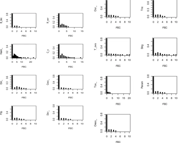
4.1.1 The presence of excessive zeroes in the data
Figure 2 show the frequency distributions of all fifteen parasite species. For all these frequency distributions, on the horizontal axis we have the faecal egg counts (FEC) and on the vertical axis we have the percentage of zero counts for di↵erent species. For all parasites species, most hosts carry a few parasites or no parasites at all while only a few hosts harbour most of the parasites (indicating the possibility of parasites being aggregated among their hosts). For example more than 80% of the hosts recorded zero counts for B. decoloratus species (Figure 3) while only 3% of host are heavily infected. There is a possibility of zero inflation due to a high proportion of zeroes in the datasets. Except for the H. hepatica species (46% zero counts), all parasite species have more than 50% zero counts. A Poisson distribution with the mean of one (will have the highest possible number of zeroes) is expected to
have below 40% zero counts. The dataset clearly has more zeroes than expected by standard count models, indicating the possibility of zero inflated distribution. 4.1.2 Variability of counts
Figure 3 shows boxplots for two parasite species, highlighting the egg count spread across some explanatory variables. Both the boxplot of C. eimeria and O. pinnata
are shown for varying factors (AGE, ANIMAL, SEX and SITE). Due to the high percentage of zeroes in data the boxplots were constructed using median intensity rather than prevalence. This means that in calculating the median for the boxplot, zeroes of uninfected hosts were excluded.
Coccidia eimeria within factor comparison indicates that angora goats and merino
sheep do not di↵er much in terms of their median faecal egg counts and that site OBW has the highest median counts compared to site OA and OHS. For Ostertagia pinnata, di↵erences are observed in terms or both age and sex median egg counts. Generally the 75th percentile of all boxplots is low (averaging around 3 egg counts), indicating that the majority of the hosts have low egg counts. This is indicative of parasite aggregation among their hosts.
Figure 4 shows boxplots for all parasite species. The boxplots were constructed using the mean prevalence, ignoring uninfected hosts with zero egg counts. Ignoring zero counts, the means and the variation of most species are similar except for; BDE
(Boophilus decoloratus), REE (Rhipicephalus evertsi evertsi), HAE (Haemonchus
contortus), CO (Coccidia Isospora) and EIM (Coccidia Eimeria). REE and HAE
are shown to have the highest means. In addition HAE has the most varying egg counts, shown in Figure 6 by the length of the boxplot being the longest. HAE is also the most abundant species (host are heavily infected by HAE compared to other species). The top extending whiskers of the boxplot shows that all egg counts are negatively skewed. The mean of these counts is far less than the median as a result a higher frequency of low counts can be expected. This is the case with most parasite counts as indicated in the previous sections. The large outliers shows the skewness of the parasite species distribution, indicating once gain that a most of the animal have zero or low egg counts while a few animal have high egg counts.
4.1.3 Characterising aggregation
Aggregation was characterised using two measures of aggregation, the variance to mean ratio and the index of discrepancy. The commonly used measure of aggregation
in literature is the variance to mean ratio, the index of discrepancy is added to validate and check the harmony between the two measures. In calculating the index of discrepancy (D), hosts in a sample are ranked from least to most infected and D
is then calculated using the formulae:
D = 1
2PNi=1⇣Pij=1xj ⌘
¯
xN(N+ 1) ,
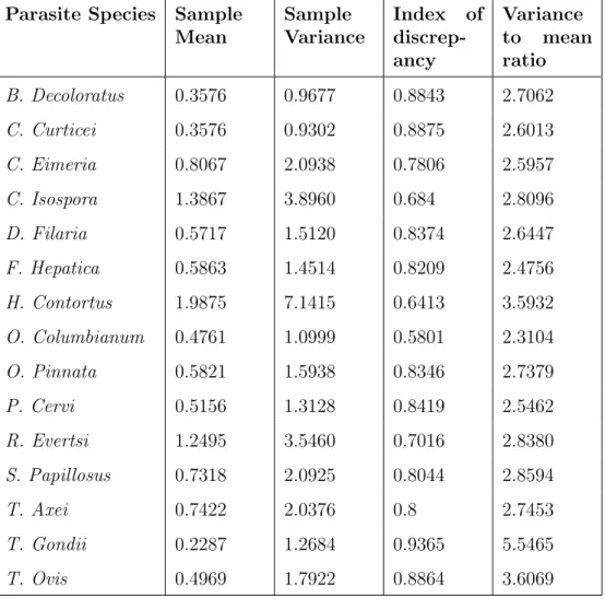
whereN is the total number of hosts in a sample andxis the egg counts on host j. The variance to mean ratio was simply calculated by taking the ratio between the sample variance and the sample mean. Table 4 shows the two calculated measures of aggregation for all parasite species.
Table 4 shows all parasite species to have a variance to mean ratio considerably greater than one. T. Gondi has the highest variance to mean ratio of 5.5465 and while
O. Columbianum has the lowest variance to mean ratio of 2.3104. This indicates that the variance is far greater than the mean and violates the Poisson assumption of equal mean and variance. As a result potential overdispersion will be factored in when formulating distributional assumptions of the parasite species. Both aggregation measures show all fifteen parasites are aggregated among their hosts. The index of discrepancy shows values close to one while the variance to mean ratio shows values greater than two. We investigate the nature of this aggregation given the covariates (AGE, ANIMAL, MONTH, SEX and SITE where the livestock were kept), by looking for any patterns of seasonality and di↵erence in aggregation given each covariate. Besides the negative binomial distribution we demonstrate other distributions that provide a good fit to over dispersed count data.
Table 4: Parasite species index of discrepancy and variance to mean ratio Parasite Species Sample
Mean Sample Variance Index of discrep-ancy Variance to mean ratio B. Decoloratus 0.3576 0.9677 0.8843 2.7062 C. Curticei 0.3576 0.9302 0.8875 2.6013 C. Eimeria 0.8067 2.0938 0.7806 2.5957 C. Isospora 1.3867 3.8960 0.684 2.8096 D. Filaria 0.5717 1.5120 0.8374 2.6447 F. Hepatica 0.5863 1.4514 0.8209 2.4756 H. Contortus 1.9875 7.1415 0.6413 3.5932 O. Columbianum 0.4761 1.0999 0.5801 2.3104 O. Pinnata 0.5821 1.5938 0.8346 2.7379 P. Cervi 0.5156 1.3128 0.8419 2.5462 R. Evertsi 1.2495 3.5460 0.7016 2.8380 S. Papillosus 0.7318 2.0925 0.8044 2.8594 T. Axei 0.7422 2.0376 0.8 2.7453 T. Gondii 0.2287 1.2684 0.9365 5.5465 T. Ovis 0.4969 1.7922 0.8864 3.6069
4.1.4 Nonparametric tests for di↵erences between factors
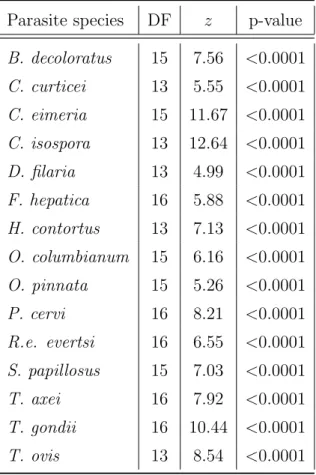
In addition to the preliminary data exploration, non parametric tests are conducted to test for di↵erences between factor medians. Parametric tests like the ANOVA assume normality, non-parametric test are based on fewer assumption as they do not assume normality. For this reason we use the Kruskal-Wallis test, which test for di↵erence in medians across multiples groups. The Kruskal-Wallis test statistic is
denoted as, H, and is calculated as; H = 12 N(N+ 1) k X j=1