Making Large Classes Small(er): Assessing the Effectiveness
Of a Hybrid Teaching Technology
Barb Bloemhof
McMaster University
and
John Livernois
University of Guelph
DISCUSSION PAPER NO. 2011-11
November 1, 2011
DEPARTMENT OF ECONOMICS AND FINANCE
UNIVERSITY OF GUELPH
GUELPH, ONTARIO
CANADA NIG 2W1
Making Large Classes Small(er): Assessing the Effectiveness Of a Hybrid Teaching Technology
Barb Bloemhof
Instructor, Department of Economics and BHSc Program, McMaster University (905) 525-9140 x 22765
(905) 521-8232 (fax) 1280 Main Street West
Hamilton, Ontario, Canada L8S 4M4 [email protected]
John Livernois (corresponding author)
Professor and Chair, Department of Economics and Finance, University of Guelph (519) 824-4120 x 56339
(519) 763-8497 (fax) 50 Stone Road East
Guelph, Ontario, Canada N1G 2W1 [email protected]
Thanks are due to the College of Management and Economics at the University of Guelph for funding this study and to Ken Rebeck for providing data. All errors are the sole responsibility of the authors.
1
Making Large Classes Small(er): Assessing the Effectiveness Of a Hybrid Teaching Technology
Abstract:
This paper examines learning outcomes in a one-semester introductory microeconomics course where contact time with the instructor was reduced by two-thirds and students were expected to view pre-recorded lectures on-line and come to class prepared to engage in discussion. Students were pre-and post-tested using the Test of Understanding in College Economics (TUCE - 4). Learning outcomes as measured by the change in test scores are found to be as good as or better than calibrating data for groups assessed using the TUCE - 4. In addition to being a more enjoyable course for the instructor, the course design can be part of a more self-directed
curriculum that uses available resources more efficiently to achieve similar learning objectives to a lecture-based introductory course.
Keywords: active learning, assessment, computer-assisted instruction, introductory microeconomics
JEL code: A22
Student enrolments in Canada have risen roughly three times faster than growth in full-time faculty over the period from 1987 to 2006 (AUCC 2008, 12 at Figure 3.2). The attendant
2
financial constraints on institutions of higher learning provide impetus for renewing the
commitment to working smarter with instructional resources. For five decades, technology has been utilized in economics to help manage and/or deliver the course (Soper 1974; Paden 1977; Siegfried and Fels 1979). Some super-large classes capture economies of scale in lecture delivery, but carry worries about the quality of learning in these environments.
Every new technology expands the hope for improved learning results. Privateer (1999) argues that teaching technologies must be deployed with a view to their efficacy in fostering learning, and not merely their value in managing the course or large class numbers (see also Creed 1997). Atkinson (2010, 57) points out that the critical factor is not how large the class is, but what is happening in that class and how the course is designed that determine whether or not the large class is conducive to active learning and learning for understanding (deep learning).
The current paper looks at using technology as a way to free up classroom contact time for more productive teaching and learning activities. Lectures were pre-recorded using screen-capture software and were made available for students to view before coming to class. As Privateer (1999, 69) suggests, recording lectures for students to view before coming to class automates the knowledge and comprehension parts of the learning objectives, freeing the instructor to change from reproduction activities to invention and intelligence-driven instructional technologies in the class time that is available. Any new technology must be expected to enhance student learning before being implemented, and the research in this paper is an exercise in quantifying that prior belief for this particular intervention in introductory
microeconomics.
The paper is organized as follows: the next section provides a brief review of the literature on technology, class size and hybrid instructional models. After that, the learning
3
context and the intervention are described. The learning outcomes measurement instrument being used in this study is the Test of Understanding in College Economics, fourth edition (TUCE - 4, Walstad et al. 2007), augmented by some additional demographic questions. We next present the results of the empirical exercise, followed by a discussion of those results. Final observations about the hybrid teaching technology are presented in the conclusions.
WHAT IS KNOWN ABOUT THE USE OF TECHNOLOGY IN LARGE INTRODUCTORY ECONOMICS CLASSES?
Principles of economics, where most students receive their first exposure to the topic, is a place where effective resource use has strong payoffs. For most students, the principles course is their first exposure to the economic way of thinking (Siegfried et al. 1991, 21) and the threshold concepts (Lucas and Mladenovic 2007, 238) that separate economists from other social
scientists. There is a significant amount of declarative knowledge and conceptual information to be learned.
Technology has long been studied as a way to provide some of that knowledge and information (Staaf 1972; Soper 1974; Allison 1976; Paden 1977; Siegfried and Fels 1979; Marlin and Niss 1982; Miller and Weil 1986; Lovell 1987; Smith and Smith 1988; Porter and Riley 1992; Hallberg 1995; Sharma et al. 2005). Russell (2010) reports a number of studies that explore the effects of technology on learning and other outcomes, with the preponderance showing no significant difference in learning outcome when compared to the traditional approach. Kulik (2003) finds small but increasing positive contribution to learning in
meta-4
analyses of a variety of computer-driven instructional technologies. Green and Gentemann (2001) find no significant difference in learning outcomes (retention or grade) between on-line versus face-to-face courses. Schenk and Silvia (1984) cite this null result as one of the reasons that computer-aided instruction (CAI) is not more widespread in the discipline. Savage (2009) also finds no statistical difference in final examination performance between students who have access to learning technology and those who did not. Navarro and Shoemaker (2000) find that a publisher’s self-paced CD-ROM version of a large introductory economics course is equal to or superior to a traditional course in terms of performance on a common examination.
Technology may be applied to leverage the economies of scale in course delivery as classes get larger, particularly in introductory course contexts. In addition, information
technology could permit the class size to be substantially reduced as it does in the hybrid course being evaluated here. Raimondo et al. (1990, 371-372) cite numerous examples from the
economics education literature of no significant difference in content knowledge performance (as measured by the TUCE) due to differences in class size, attributing this to the idea that only the lower-level cognitive skills of recall and comprehension are emphasized in introductory courses. More recently, Arias and Walker (2006) find that increasing class size does have a significant negative impact in a study that controls for student ability. There may also be deleterious impacts as class size increases at the primary education level (Sims 2009).
Bedard and Kuhn (2008) find large and significant reduction of instructor effectiveness as reported in student evaluations of teaching, so clearly students notice some differences in the environment as class size increases, although instructor effectiveness is not the same as student performance. Tay (1994, 291) emphasizes a number of student-specific characteristics that are important to learning outcomes, particularly aptitude and effort. Dobkin et al. (2010) find that
5
attendance explains a significant portion of the final exam performance, apparently with no cost to student performance in other classes.
The works discussed so far tend to treat technology as substitute for lecturing, to “(make) the same course information available to a wide audience of information consumers” (Privateer 1999, 68). Creed (1997, 4) observes that technologies that improve presentation of material are not inherently organized around student learning. Some uses of technology may be at cross purposes with a learner-centered approach, even though applications of technology are often advocated as a way to improve learning. As Maki et al. (2000, 230) say so succinctly, “[t]here is no pedagogical rationale for teaching in the lecture format;” they advocate instead taking Barr and Tagg’s (1995) advice to focus on the learning rather than the teaching that goes on. Barr and Tagg’s learning paradigm justifies breaking away from habitual methods of teaching if the change can better support learning.
The challenge, then, is to explore ways to capitalize on the special features of technology that can be harnessed to foster different and better learning (for example, Schwerdt and
Wupperman 2011). Maki et al. (2000) report that in their small introductory psychology classes, while performance is significantly better with on-line teaching and learning activities augmenting the readings, students were more enthusiastic about the course content in the lecture version of the course. The performance result may be due to differences in content mastery because students in the on-line version of the course are required complete two quizzes per week at 80% or better.
Siegfried and Fels (1979, 942) distinguish between CAI and computerized study management systems (which give periodic diagnostic quizzes and help students optimize their studying effort). For example, technology could make mastery testing available as a
6
complement to the lecture version of the course in Maki et al. (2000), with likely positive effects on performance. Smeaton and Keogh’s (1999) experiment misses an opportunity to enhance learning because they do not redeploy the time freed up by providing the content digitally.
By contrast, Day et al. (2004) do make new uses of the time freed up by delivering content using technology. Students come to class having viewed the web lectures in advance, so that class time provides the opportunity to “answer questions, discuss difficult subject material, and engage in more active, authentic learning activities” (Day et al. 2004, 3). Marlin and Niss (1982) similarly use class time made available by a self-paced, computer-managed course for discussion and other teaching and learning activities hosted by the instructor. In addition, Marlin and Niss complement these practices with mastery learning, which is known to be useful for maximal learning impact (Lalley and Gentile 2009). The expectation that students are
responsible for preparing for class is a valuable self-management norm to incorporate into the learning environment.
DESCRIPTION OF THE INTERVENTION
At the host institution, Introductory Microeconomics has traditionally been taught as a
lecture-style course with enrolments ranging from 300 to 600.1 In 2010, the instructor of one
section of about 300 students changed the format of the course to a hybrid style in which pre-recorded lectures were streamed over the internet. In the second offering of this new format, a pre-and post-test was administered to students in order to assess the effectiveness of this hybrid style. The prior expectation from the literature was that “students viewing web lectures should
7
retain at least as much as students viewing traditional lectures” (Day et al. 2004, 2; italics in
original).
Lectures were pre-recorded using Camtasia Studio © screen recording software. Each
lecture is roughly one hour in length and usually covered one topic. Students could view the lectures from any location with internet access whenever and as often as they like. Fifteen topics made up the content of the course.
In the first week, the class was divided into three groups and thereafter each group attended just one, one-hour class per week (as compared to three, one-hour lectures in the traditional lecture course format). Consequently, class size was one-third of the usual size. Students were asked to be familiar with the material before coming to class by reading the textbook and watching the videos and taking notes as they would in a regular lecture. The class time was used to engage students in active learning activities such as discussion of applications of theory to current or historical events, group work on problems, and activities such as playing prisoner-dilemma and bidding games.
The object of the research is to evaluate the effectiveness of the hybrid course structure
relative to the traditional lecture-style format. This is done by using the standardized Test of
Understanding of College Economics, fourth edition (TUCE – 4) (Walstad et al. 2007). TUCE – 4 is a multiple-choice test that has been administered as a pre- and post-test to 3255 students under 71 instructors at 43 colleges and universities in the United States. It provides reliable norming data against which to compare the performance of the students in the hybrid course being evaluated.
In the course being evaluated, the pre-test was administered to the entire class of students in the first week of classes. A number of supplementary questions were appended to the TUCE –
8
4 test instrument to provide demographic and other information. In the last week of classes, the same test was administered again. Students were told that the tests would not count, but that they provided useful practice because they were very similar in format to the midterm and final assessments. Students were not aware that the same practice test would be given at the end of semester.
RESULTS
Three hundred and three students wrote the pre-test; due to attrition and absenteeism, 123
students wrote the post-test.2 Some respondents did not answer all of supplemental questions.
We analyze the test results by comparing the mean test scores to the norming data using the 123 matched test scores first, and then we analyze characteristics that may have influenced the test scores using only the 233 observations for the pre-test and the 86 observations for the post-test for which there is a complete set of responses to the supplemental questions. First, we report the sample distributions of responses.
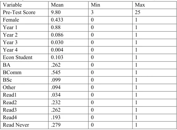
Table 1 contains summary statistics for the 233 students that returned complete questionnaires. The average pre-test score was 9.80 out a possible 30, almost identical to the overall average of 9.79 for all 303 students. The difference is not statistically different. The remaining variables in Table 1 are binary variables and as such, the mean values can be interpreted as proportions. Table 1 shows that 43.3 % of the students writing the pre-test were female, 88% were first-year students, 10.3% declared themselves to be economics majors, 54.5% were Bachelor of Commerce (BComm) students, for whom the course is required, 26.2% were Bachelor of Arts students for some of whom the course is required, and the remaining 19% were from other degree programs for whom the course is not required. About 3.4% said they read
9
economics news or magazine articles at least once per day (Read1), another 23.2% do so at least once per week (Read2), 26.2% do so once per month (Read3), 19.3% do so once per year (Read4) and the remaining 27.9% of the students writing the pre-test said they never read economics news or magazine articles.
[INSERT TABLE 1 ABOUT HERE]
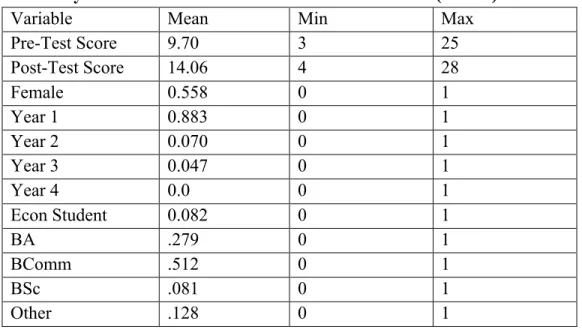
Table 2 contains summary information about the 86 students included in Table 1 that also took post-test. Most of the characteristics are very similar between Tables 1 and 2. For example, the pre-test average score for those students that also wrote the post-test is a bit lower (9.7) but the difference is not statistically significant. The one difference that stands out is that the
proportion of female students writing the post-test was 55.8% compared to 43.3% at the pre-test. In this sample, females were more likely than males to show up for the post-test in the last week of semester.
[INSERT TABLE 2 ABOUT HERE]
Comparison of Observed Class to TUCE – 4 Norming Data:
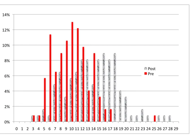
Figure 1 shows the frequency distributions of matched scores (out of 30) for the pre-test and post-test. As one would hope and expect, the distribution visibly shifts to the right after a semester of instruction. At the very bottom of the distribution (scores of 3 and 4) there was no change. However, for all higher test scores, the post-test distribution moves to the right. In particular, the upper end of the distribution became substantially more populated which suggests that there was a subset of students that learned a good deal of economics during the semester.
10
Tables 3a – 3c report the average scores achieved for the matched sample of students that wrote both the pre-test and post-test in the class (N = 123), for the complete set of norming data from TUCE – 4 (N = 3255) and for the subset of norming data from TUCE – 4 that apply only to doctoral/research universities. The latter set of norming data is included because the observed class is from a research-intensive university with a doctoral program.
[INSERT TABLES 3a – 3c ABOUT HERE]
In Table 3a, the pre-test average score for the observed class (9.97) is compared to the pre-test average score for the complete set of observations in the norming data (9.39) and for the subset of observations at universities classified by Walstad et al. (2007) as doctoral/research (9.73). The last column of the table reports the probability values for the hypothesis that the mean is equal to (respectively) the overall TUCE – 4 mean and the TUCE – 4 doctoral/research university mean under the assumption that all populations have the same variance. The
hypothesis that the mean of 9.97 at the observed class is equal to the overall TUCE – 4 mean of 9.39 is rejected at the 3% level but we cannot reject the hypothesis that the mean score of students in the observed class is equal to the TUCE – 4 mean for doctoral universities of 9.73.
Table 3b provides similar information for the post-test scores with similar results. The mean on the post-test is higher than the overall TUCE – 4 mean at level of significance below 1%. Comparing the TUCE – 4 doctoral university mean of 13.44 to the mean of 13.98, we cannot reject the hypothesis they are equal (p = 0.11).
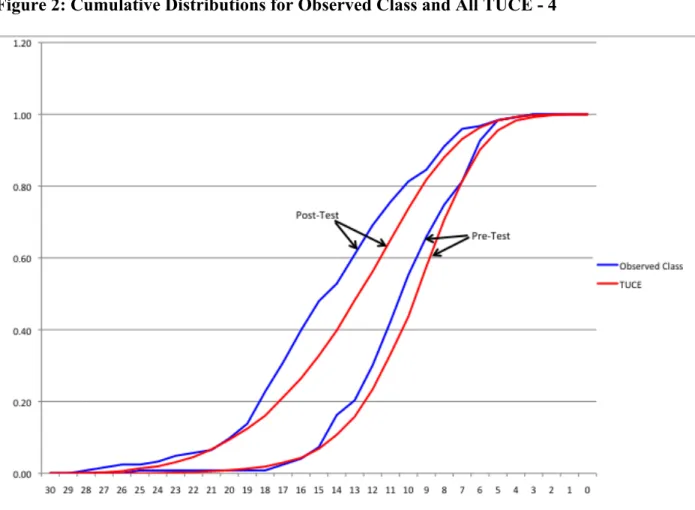
Figure 2 shows the cumulative distributions on the pre- and post-test for the set of
respondents from the observed class and for the overall TUCE – 4 norming data.3 For both the
pre- and post-test, the distribution lies to the left of its TUCE – 4 counterpart indicating that not just the average scores, but almost the entire distribution of scores was higher than the overall
11
TUCE – 4. In addition, the leftward shift of the post-test distribution relative to its
corresponding pre-test distribution shows that there was across-the-board improvement for both. Our interest at this stage, however, is in comparing the size of the leftward shift in the
cumulative distribution to the leftward shift in the TUCE – 4 norming data cumulative
distribution. An easier but equivalent way to see this is to compare the difference between the post-test distributions for the observed class and for TUCE – 4 to the difference between the pre-test distributions for respondents from the observed class and TUCE – 4. Visually, Figure 2 shows a larger leftward shift for the observed class sample, suggesting that the hybrid model led to superior learning than in the TUCE – 4 norming data.
[INSERT FIGURE 2 ABOUT HERE]
Next, we test the hypothesis that the average of the change scores is higher in respondents from the observed class than in the TUCE – 4 data. Table 3c compares the mean change scores. On average, the scores improved by 4.01 in the matched sample of 123 students, whereas it increased by 3.38 and 3.71 respectively in the complete set of TUCE – 4 scores and the TUCE – 4 doctoral/research university scores. It is encouraging that the change score is higher than either of the norming data change scores, even though the pre-score in the observed class started higher than the TUCE pre-score. This confirms our prior belief that the hybrid teaching methodology did not disadvantage the students in terms of ability to perform on standardized multiple-choice questions and, in fact, may have led to superior learning as measured by the change-scores.
The last column of Table 3c shows the probability values for the hypothesis that the mean change scores are equal against the alternative hypothesis that the observed class mean change-score is higher. We cannot reject the hypothesis that the observed mean is equal to the TUCE – 4 mean for the doctoral/research universities, which supports the notion that these are similar
12
caliber institutions and the doctoral/research university subset of TUCE – 4 is the correct comparison data. However, we reject the hypothesis that the mean change score is equal to the mean change score for the complete TUCE – 4 data at the 9.3% level.
It is encouraging to find that the hybrid style course in the observed class is associated with higher test scores on both the pre-test and post-tests and a larger change-score than the overall TUCE – 4 results and those for the subset of doctoral/research universities. However, we are cautious about drawing firm conclusions for two reasons. First, this conclusion is statistically significant for the comparison against the overall TUCE – 4 data but not for the comparison against the doctoral/research universities. Even though the observed class’s change-score is higher, at 123 the sample size is not large enough to allow us to conclude that the difference is not due to chance. Second, the comparison of mean test scores on the post test and for the change-scores between the observed class and the norming data is meaningful only if whatever sample selectivity biases exist are similar for all the post-test samples. Since we have no way of testing this, we can only be cautious about generalizing the interpretation outside of the sample from the observed class.
Effects of Characteristics on Performance
Table 1 shows that almost all the students were in their first year, indeed their first week, of university when they wrote the pre-test. We expected them to know very little of the
terminology of economics and very little about microeconomic theory, even at a very basic level. Very few respondents said that they had taken an economics course before, and therefore, we do not include this variable in our analysis.
13
We hypothesize that the kth student’s performance on the pre-test can be explained by the
following linear model:
(1)
where the pre-test score is a positive integer less than or equal to 30, N is the number of students
that wrote the pre-test, and the xivariables are: Female (1 if female), Year2 (1 if enrolled in
second year), Year3 (1 if in third year), Year4 (1 if in fourth year), ECON (1 if an economics major), BComm (1 if in the Bachelor of Commerce program), BSc (1 if in the Bachelor of Science program), Other (1 if in some other program), Read1 (1 if reads economics news or magazine articles daily), Read2 (1 if reads at least once per week), Read3 (1 if reads at least once per month), Read4 (1 if reads at least once per year). We have no prior expectation for the effect of gender on test outcomes. However, we expect that higher-year students (Year2, Year3 and Year 4), students that have declared their major as economics (ECON), and students that read economics news articles (Read1, Read2, Read3, Read4) are likely to perform better on the
pre-test. A priori, Bachelor of Commerce (BComm) students could perform better than Bachelor of
Arts (BA) students (the excluded dummy) because of an interest in business; on the other hand, most of them are taking it only because it is required and so may have less interest in the analytical approach inherent in economics courses. Finally, we have no prior belief about whether Bachelor of Science students will perform better or worse than BA students.
Next, we hypothesize that the jth student’s performance on the post-test can also be
14
where NMis the matched number of students (that wrote both tests). The maintained hypothesis
is that the characteristics in the supplementary questions affect performance on the pre-test and on the post-test, although the magnitudes may differ. We define the change score as the difference between the post- and pre-test scores:
and therefore, the change score can be explained by the following linear model:
(2)
where
It is conceivable that the characteristics variables have the same impact on both the pre- and post-tests and hence cancel out in the change-score regression. On the other hand, if some of these characteristics variables act as proxies for the unobservable characteristics that measure learning ability and outcomes (such as how many hours per week the student devoted to the course and how motivated to learn was the student), then the effects will not cancel out in the change-score regression. These are testable hypotheses.
Sample selection bias is a concern for the change-score model because we do not have change score data for those students that did not write the post-test. Therefore, a standard
15
Heckman sample selection correction procedure is performed in which a probit model is first estimated to ascertain the determinants of the likelihood of writing the post-test. The estimated inverse Mills ratio is then included as an additional explanatory variable in the above OLS regression of the change score (for those students who wrote both tests). The explanatory variables included in each regression are explained in the results table.
Table 4 shows the results of the OLS regression model (1). The model explains a very small proportion of the variation in pre-test scores (R-squared = 0.069) but the hypothesis that all slope coefficients are zero is rejected at less than the 1% level. The implication is that we can reject the hypothesis that students were just randomly guessing at answers. In fact, one can easily reject the hypothesis that the overall average score (9.80) is not different from 7.5, the expected average score if students were randomly guessing.
[INSERT TABLE 4 ABOUT HERE]
Table 4 shows that females were likely to score about a point lower than males, all else equal and this result is statistically significant at the 1.4% level. Senior students are more likely to score higher than first-year students. For example, third-year students score nearly two points higher (but this is statistically significant only at the 11.5% level) and fourth year students score higher by a huge 5.38 points, a result that is statistically significant at the 8.6% level. Bachelor of Commerce students were likely to score 0.862 points lower than BA students (the excluded dummy), statistically significant at the 8% level, and students that read economics news articles on a daily basis (Read1) are likely to score 2.33 points higher than students that never read economics news articles. This result is large and is statistically significant at the 4.7% level.
The results shown in Table 4 are interesting in that they provide an indication of what characteristics are likely to lead to a greater or lesser ability for students that have never studied
16
economics to provide correct responses. It is especially interesting to see whether any of these characteristics also have a significant effect on learning as measured by the change score or whether the effects cancel out between the post- and pre-test. We turn to these results next.
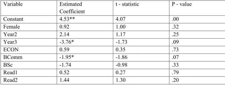
We begin by presenting the results of the estimation of model (2) without selectivity correction as a point of comparison for the model when it is corrected for sample selection bias. Observations are restricted to the 86 students that wrote both tests and provided answers to the questions about characteristics. Table 5 presents the results. In this model, the change in test scores, meant to measure learning over the course of the semester, is regressed against
characteristics variables. For consistency with the following models, we dropped characteristics variables for which there were few observations (in the smaller sample) and no statistically significant influence.
[INSERT TABLE 5 ABOUT HERE]
Although females performed lower on the pre-test, Table 5 shows that they had a positive overall change in performance, though the difference is not statistically significant. Third-year students achieved a much lower change score (3.76 points lower), significant at the 9% level. However, only 4.7% of the students that wrote both tests were in third year. BComm students achieved a smaller improvement in test scores (1.74 points less) than BA students, significant at the 7% level. Finally, the variable Read1 (read economics/business news at least once per day), which was a significant predictor of superior performance on the pre-test, has no significant effect on learning which may be due to similar effects of this variable in both the pre- and post-tests that cancelled out in the change score.
The results in Table 5 are likely to be biased due to sample selectivity. It is possible that students who opted out of the post-test sample have different characteristics than the students
17
that selected in. In particular, it has already been noted that the gender-composition was very different on the post-test than it was on the pre-test. To compensate for this, we run a standard
Heckman correction. We define the dummy variable D = 1 if both tests are written and D = 0 if
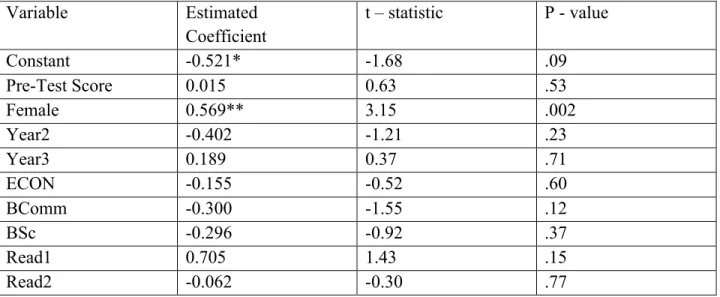
just the pre-test is written. We hypothesize that the likelihood that a student selects into the post-test sample is a linear function of the characteristics variables listed in Table 6 which shows the results of the probit regression.
[INSERT TABLE 6 ABOUT HERE]
We include all the explanatory variables in the probit regression as we used in the change-score regression and in addition include one more that is excluded from the latter: the pre-test score. Our expectation is that students with higher pre-test scores are more likely to write the post-test.
Table 6 shows that the pre-test score does have a positive coefficient as expected but it is small and not statistically significant. On the other hand, females were much more likely to write the post-test than males, an effect that is strongly significant (p < 1%). Commerce students appear to be less likely to write the post-test but the result is not significant below the 12% level. None of the other characteristics had a statistically significant influence on the dependent
variable.
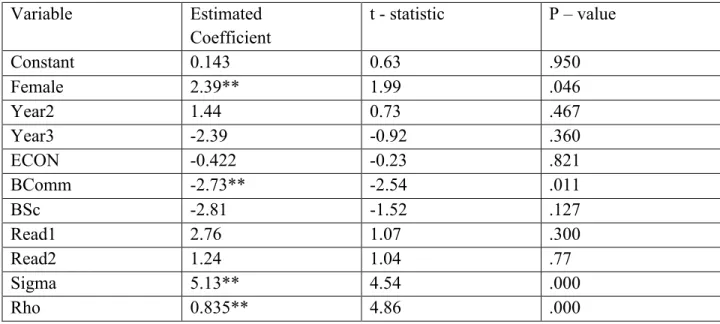
The inverse Mills ratio is calculated for the 86 observations for which the post-test was written and included as an explanatory variable in the OLS regression to explain the change score. The results are shown in Table 7. The first result to note is that sample selection bias is present and statistically significant as indicated by the very low probability values on the
18
surprising given the results so far that have indicated both that females performed worse than males on the pre-test but were much more likely to be present at the post-test.
[INSERT TABLE 7 ABOUT HERE]
Two results in particular stand out in Table 7. First, females now show a statistically significant and much larger improvement in scores compared to males. Females improved their score by 2.39 points more than did males, all else equal. Apparently, females learned more economics than males over the course of the semester. On the other hand, Bachelor of
Commerce students performed worse than Bachelor of Arts students. All else equal, Bachelor of Commerce students had a test score improvement that was 2.73 points less than that for Bachelor of Arts students, significant at the 1% level. These results indicate that the coefficients in Table 5 are biased downwards due to the effect of sample selectivity.
CONCLUSIONS
The purpose of this paper was to evaluate the effectiveness of the hybrid teaching
technology used in Introductory Microeconomics. The prior expectation from the literature was that the hybrid teaching technology should result in retention of material that is no worse than traditional lectures (Day et al. 2004, 2). In addition, we anticipated that the reduction of the class size by two-thirds and the use of the remaining class time for more active learning would have enhanced learning (Lalley and Gentile 2009; Marlin and Niss 1982).
To evaluate the effectiveness of this teaching approach, students were pre- and post-tested using the TUCE – 4 multiple-choice test and the results were compared to the average test results of the overall sample published in the TUCE – 4 manual (3255 students at 43 colleges
19
and universities in the US) and to the average test results from the subsample of doctoral/research universities (758 students at 14 universities in the US).
Compared to the TUCE – 4 norming data, the students tested in the observed hybrid course performed better on the pre-test, better on the post-test, and achieved a larger
improvement from pre- to post-test. This is true compared to both the students in the full TUCE sample of 3255 students and in the subsample of 758 students at doctoral/research universities. However, the differences are statistically significant only for the comparison against the full TUCE sample of 3255 that includes undergraduate teaching colleges as well as doctoral/research universities. For the comparison to the doctoral/research universities, the scores in the observed class are very similar to the norming data for doctoral/research universities.
The test results for students in the observed hybrid course were analyzed to determine whether any student characteristics reported in the supplementary questions were statistically significant predictors of performance. Females scored lower than males on the pre-test, senior students scored higher than first-year students, Bachelor of Commerce students scored lower than Bachelor of Arts students and students who read economics news articles frequently scored higher than students who never read economics news articles. However, many of these effects disappeared when we considered the determinants of the change in test scores (post-test minus pre-test) presumably because they affected the post-test performance in the same way they affected the pre-test performance. Two characteristics that did have a statistically discernable effect on the change-score were gender (test scores for females improved much more than those for males) and Bachelor of Commerce students whose test scores not only started lower but improved less than those for Bachelor of Arts students. One hypothesis that could explain this finding is that perhaps many of these students are not interested in understanding economics and
20
so take a surface learning approach with a course they are required to take as part of their program. In any case, neither of these statistically significant findings would change the teaching approach in the course.
Therefore, the prior expectation that learning outcomes would be at least as good in the hybrid course is borne out in the empirical results. The additional expectation that the reduced class size and more active learning would reinforce engagement and, therefore, performance on the post-test, received mixed results. One cannot reject the hypothesis that the superior change-score we found among the observed class of students is due to chance. However, given the high degree of attrition between the pre-and post-test, it is clear that only about one-third of the class benefitted from the active learning opportunities in the hybrid teaching technology. The high degree of attrition is indeed a concern in our evaluation of the effectiveness of the hybrid teaching technology. One of the primary objectives of moving away from the traditional large-class lecture format was to provide students with more engaging in-large-class learning activities. We need to know more about the true reasons for non-attendance, and address them in order to achieve this objective for everyone enrolled in the class.
21
NOTES
1The intervention took place at a medium-sized research-intensive department with a PhD
program that is ranked 15th of the 41 economics programs in the top 25% in Canada by RePEc as of April 2011.
2Attendance was low for most of the semester. Some students may have felt that the on-line
lectures were a substitute for class time. In addition, written evaluations revealed that some students did not attend classes because they were not prepared for the discussion topics and therefore thought they had nothing to gain by attending class.
REFERENCES
Allison, E. K. 1976. The Use of Video in Economic Education. Journal of Economic Education
8(1): 27-36.
Arias, J.J. and D. M. Walker. 2006. Additional Evidence on the Relationship between Class Size
and Student Performance. Journal of Economic Education 35(4): 311-329.
Association of Universities and Colleges of Canada (AUCC). 2008. Trends in Higher
Education, Volume 3: Finance. Ottawa: AUCC.
http://www.aucc.ca/_pdf/english/publications/trends_2008_vol3_e.pdf. (accessed April 15, 2011).
Atkinson, M. 2010. Teaching Large Classes. In The Dynamic Classroom: Engaging Students
in Higher Education, ed. C. Black, 57-67. Madison, WI: Atwood Publishing.
Barr, R. B. and J. Tagg. 1995. From Teaching to Learning - A New Paradigm for Undergraduate
Education. Change (November-December): 13-25.
Bedard, K. and P. Kuhn. 2008. Where Class Size Really Matters: Class Size and Student Ratings
of Instructor Effectiveness. Economics of Education Review 27(3): 253-265.
Creed, T. 1997. Powerpoint, No! Cyberspace, Yes! National Teaching and Learning Forum
6(4) (May). http://www.ntlf.com/html/pi/9705/creed_1.htm (accessed April 5, 2011). Day, J. A., J. D. Foley, R. Groeneweg, and C. A. P. G. Van der Mast. 2004. Enhancing the
Classroom Learning Experience with Web Lectures. GVU Technical Report: GIT-GVU-04-18.
23
Dobkin, C., R. Gil and J. Marion. 2010. Skipping Class in College and Exam Performance:
Evidence from a Regression Discontinuity Classroom Experiment. Economics of Education
Review 29(4):566-575.
Green, R. and K Gentemann. 2001. Technology in the Curriculum: An Assessment of the Impact of On-Line Courses. George Mason University Office of Institutional Assessment. https://assessment.gmu.edu/Results/Other/2000/Eng302/Eng302Report.pdf (accessed April 28, 2011).
Hallberg, M. C. 1995. Policy: A Computer Program for Student Use in Courses on Economic
Policy. Journal of Economic Education 26(4): 314-323.
Kulik, J. A. 2003. Effects of Using Instructional Technology in Colleges and Universities: What
Controlled Evaluation Studies Say. Final Report. SRI Project Number P10446.003 (December).
Arlington, VA: SRI International.
http://sri.com/policy/csted/reports/sandt/it/Kulik_IT_in_colleges_and_universities.pdf (accessed April 5, 2011).
Lalley, J. P. and J. R. Gentile. 2009. Classroom Assessment and Grading to Assure Mastery.
Theory Into Practice 48(1): 28-35.
Lovell, M. C. 1987. CAI on PCs – Some Economic Applications. Journal of Economic
Education 18(3): 319-329.
Lucas, U. and R. Mladenovic. 2007. The Potential of Threshold Concepts: An Emerging
Framework for Educational Research and Practice. London Review of Education 5(3): 237-248.
Maki, R. H., W. S. Maki, M. Patterson and P. D. Whittaker. 2000. Evaluation of a Web-based Introductory Psychology Course: I. Learning and Satisfaction in on-line versus Lecture Courses.
24
Marlin, J. W., Jr., and J. F. Niss. 1982. The Advanced Learning System, a Computer-managed,
Self-paced System of Instruction: An Application in Principles of Economics. Journal of
Economic Education 13(2): 26-39.
Michael, J. 2006. Where's the evidence that active learning works? Advances in Physiology
Education 30: 159-167.
Miller, J. and G. Weil. 1986. Interactive Computer Lessons for Introductory Economics: Guided
Inquiry – From Supply and Demand to Women in the Economy. Journal of Economic Education
17(1): 61-68.
Navarro, P. and J. Shoemaker. 2000. Performance and perceptions of distance learning in
cyberspace. American Journal of Distance Education 14(2): 15-35.
Paden, D. W. 1977. The Use of Television in Teaching Basic Economics at the College Level.
Journal of Economic Education 9(1): 21-27.
Porter, T. S. and T. M. Riley. 1992. CAI in Economics: What Happened to the Revolution?
Journal of Economic Education 23(4). 374-378.
Privateer, P. M. 1999. Academic Technology and the Future of Higher Education: Strategic
Paths Taken and Not Taken. Journal of Higher Education 70(1): 60-79.
Raimondo, H. J., L. Esposito and I. Gershenberg. 1990. Introductory Class Size and Student
Performance in Intermediate Theory Courses. Journal of Economic Education 21(4): 369-381.
Russell, T. L. 2010. The No Significant Difference Phenomenon. No Significant Difference
presented by WCET (Wiche Cooperative for Educational Technologies). http://www.nosignificantdifference.org/ (accessed April 5, 2011).
Savage, S. J. 2009. The Effect of Information Technology on Economic Education. Journal of
25
Schenk, R. and J. E. Silvia. 1984. Why has CAI not been more successful in economic
education: A Note. Journal of Economic Education 15(3): 239-42.
Schwerdt, G. and A. C. Wuppermann. 2011. Is Traditional Teaching Really All That Bad? A
Within-Student Between-Subject Approach. Economics of Education Review 30(2): 380-389.
Sharma, M. D., J. Khachan, B. Chan and J. O’Byrne. 2005. An Investigation of the Effectiveness
of Electronic Classroom Communications systems in Large Lecture Classes. Australasian
Journal of Educational Technology 21(2): 137-154. http://ascilite.org.au/ajet/ajet21/sharma.html (accessed March 23, 2011).
Siegfried, J. J., R. L. Bartlett, W. L. Hansen, A. C. Kelley, D. N. McCloskey, and T. H.
Tietenberg. 1991. The Economics Major: Can and Should We Do Better than a B-? American
Economic Review 81(2): 20-25.
Siegfried, J. J. and R. Fels. 1979. Research on Teaching College Economics: A Survey. Journal
of Economic Literature 17(3): 923-69.
Sims, D. 2009. Crowding Peter to educate Paul: Lessons from a Class Size Reduction
Externality. Economics of Education Review 28(4): 465-473.
Smeaton, A. F. and G. Keogh. 1999. An Analysis of the Use of Virtual Delivery of
Undergraduate Lectures. Computers and Education 32(1): 83-94.
Smith, L. M., and L.C. Smith, Jr. 1988. Teaching Microeconomics with Microcomputer
Spreadsheets. Journal of Economic Education 19(4): 363-382.
Soper, J. C. 1974. Computer-assisted Instruction in Economics: A Survey. Journal of Economic
Education 6(1): 5-29.
Staaf, R. J. 1972. Student Performance and Changes in Learning Technology In Required
26
Tay, R. S. 1994. Students’ Performance in Economics: Does the Norm Hold Across Cultural
and Institutional Settings? Journal of Economic Education 25(4): 291-301.
TechSmith. 2011. Camtasia Studio. http://www.techsmith.com/camtasia/ (accessed April 5,
2011).
Walstad, W. B., M. Watts and K. Rebeck. 2007. Test of Understanding in College Economics:
27
Table 1: Summary Statistics for Students who Wrote the Pre-Test (N=233)
Variable Mean Min Max
Pre-Test Score 9.80 3 25 Female 0.433 0 1 Year 1 0.88 0 1 Year 2 0.086 0 1 Year 3 0.030 0 1 Year 4 0.004 0 1 Econ Student 0.103 0 1 BA .262 0 1 BComm .545 0 1 BSc .099 0 1 Other .094 0 1 Read1 .034 0 1 Read2 .232 0 1 Read3 .262 0 1 Read4 .193 0 1 Read Never .279 0 1
28
Table 2: Summary Statistics for Students who Wrote Both Tests (N = 86)
Variable Mean Min Max
Pre-Test Score 9.70 3 25 Post-Test Score 14.06 4 28 Female 0.558 0 1 Year 1 0.883 0 1 Year 2 0.070 0 1 Year 3 0.047 0 1 Year 4 0.0 0 1 Econ Student 0.082 0 1 BA .279 0 1 BComm .512 0 1 BSc .081 0 1 Other .128 0 1
29
Table 3: Analysis of Test Scores
Table 3a: Pre-Test Scores
Pre-Test: Pre-Test: All
TUCE – 4
Pre-Test TUCE – 4 Doctoral University
P values for diff in means
Mean 9.97 9.39 9.73 .03, .48
St. Dev. 3.38 3.32 3.50
N 123 3255 758
Table 3b: Post-Test Scores
Post-Test: Post-Test: All
TUCE – 4
Post-Test TUCE – 4 Doctoral University
P values for diff in means
Mean 13.98 12.77 13.44 .003, .11
St. Dev. 4.82 4.68 4.45
N 123 3255 758
Table 3c: Change Scores
Change: Change: All
TUCE – 4
Change: TUCE – 4 Doctoral University
P values for diff in means
Mean 4.01 3.38 3.71 .093, .45
St. Dev. 4.08 4.42 4.45
N 123 3255 758
The standard deviations for the TUCE - 4 change scores are not available in Walstad et al. (2007). We are grateful to Ken Rebeck for providing them to us.
30
Table 4: Dependent Variable Pre-Test Score Variable Estimated Coefficient t-statistic p-value Constant 10.35** 17.78 .000 Female -1.06** -2.49 .014 Year2 .543 0.71 .477 Year3 1.94 1.58 .115 Year4 5.38* 1.72 .086 ECON .870 1.23 .206 BComm -0.862* -1.76 .080 BSc -0.738 -0.92 .357 Other -0.212 -0.27 .787 Read1 2.33* 2.00 .047 Read2 0.131 0.23 .820 Read3 0.196 0.35 .723 Read4 0.465 0.77 .440
Standard error of regression: 3.03 Adjusted R-squared: .069
31
Table 5: OLS Results: Dependent Variable = Change Score
Variable Estimated Coefficient t - statistic P - value Constant 4.53** 4.07 .00 Female 0.92 1.00 .32 Year2 2.14 1.17 .25 Year3 -3.76* -1.73 .09 ECON 0.59 0.35 .73 BComm -1.95* -1.86 .07 BSc -1.74 -0.98 .33 Read1 0.52 0.27 .79 Read2 1.44 1.30 .20
Standard error of regression: 3.94 Adjusted R-squared: .044
32
Table 6: Probit Results: Dependent Variable = D (1 if both pre- & post-test written)
Variable Estimated Coefficient t – statistic P - value Constant -0.521* -1.68 .09 Pre-Test Score 0.015 0.63 .53 Female 0.569** 3.15 .002 Year2 -0.402 -1.21 .23 Year3 0.189 0.37 .71 ECON -0.155 -0.52 .60 BComm -0.300 -1.55 .12 BSc -0.296 -0.92 .37 Read1 0.705 1.43 .15 Read2 -0.062 -0.30 .77 N = 233
33
Table 7: OLS Results with Heckman Correction: Dependent Variable = Change Score
Variable Estimated Coefficient t - statistic P – value Constant 0.143 0.63 .950 Female 2.39** 1.99 .046 Year2 1.44 0.73 .467 Year3 -2.39 -0.92 .360 ECON -0.422 -0.23 .821 BComm -2.73** -2.54 .011 BSc -2.81 -1.52 .127 Read1 2.76 1.07 .300 Read2 1.24 1.04 .77 Sigma 5.13** 4.54 .000 Rho 0.835** 4.86 .000 N = 86
34
Figure 1: Pre- and Post-Test Frequencies for Matched Sample (N = 86)
0% 2% 4% 6% 8% 10% 12% 14% 0 1 2 3 4 5 6 7 8 9 10 11 12 13 14 15 16 17 18 19 20 21 22 23 24 25 26 27 28 29 Post Pre
35