Final Technical Report TransNow Budget No. 61-6020
Occlusion Robust and Environment Insensitive
Algorithm for Vehicle Detection and Tracking Using
Surveillance Video Cameras
by
Yinhai Wang, PhD Yegor Malinovskiy Yao-Jan Wu
Associate Professor Graduate Research Assistant Graduate Research Assistant Department of Civil and Environmental Engineering
University of Washington Seattle, Washington 98195-2700
Sponsored by
Transportation Northwest (TransNow) University of Washington
135 More Hall, Box 352700 Seattle, Washington 98195-2700
in cooperation with
U.S. Department of Transportation Federal Highway Administration
Report prepared for:
Transportation Northwest (TransNow) Department of Civil and Environmental Engineering
129 More Hall
University of Washington, Box 352700 Seattle, Washington 98195-2700
TECHNICAL REPORT STANDARD TITLE PAGE
TNW2008-12 2. GOVERNMENT ACCESSION NO. 3. RECIPIENT’S CATALOG NO. 4. TITLE AND SUBTITLE
Occlusion Robust and Environment Insensitive Algorithm for Vehicle Detection and Tracking Using Surveillance Video Cameras
5. REPORT DATE
December 31, 2008 6. PERFORMING ORGANIZATION CODE
7. AUTHOR(S)
Yinhai Wang, Yegor Malinovskiy, and Yao-Jan Wu
8. PERFORMING ORGANIZATION REPORT NO. TNW2008-12
9. PERFORMING ORGANIZATION NAME AND ADDRESS
Transportation Northwest Regional Center X (TransNow) Box 352700, 123 More Hall
University of Washington Seattle, WA 98195-2700
10. WORK UNIT NO.
11. CONTRACT GRANT NO. DTRT07-G-0010
12. SPONSORING AGENCY NAME AND ADDRESS 13. TYPE OF REPORT AND PERIOD COVERED Research Report
14. SPONSORING AGENCY CODE 15. SUPPLEMENTARY NOTES
This study was conducted in cooperation with the University of Washington and the US Department of Transportation
16. ABSTRACT
With the decreasing price of video cameras and their increased deployment on roadway networks, traffic data collection through video imaging has grown in popularity. Numerous vehicle detection and tracking algorithms have been developed for video sensors. However, most existing algorithms function only within a narrow band of environmental conditions and occlusion-free scenarios. In this study, a novel video-based vehicle detection and tracking algorithm is developed for traffic data collection under a broader range of environmental factors and traffic flow conditions. This algorithm employs a scan-line approach to generate spatio-temporal maps representing vehicle trajectories. Vehicle trajectories are then extracted by determining the Hough lines of the obtained ST-maps and grouping the Hough lines using the connected component analysis method. The algorithm is implemented in C++ using
OpenCV and BOOST C++ libraries and is capable of operating in real-time. Over five hours of surveillance video footage was used to test the algorithm. Detection count errors ranged from under 1% in the relatively simple situations to under 15% in highly challenging scenarios. This result is very encouraging because the test video sets were taken under demanding conditions that ordinary video image processing algorithms cannot deal with. This implies that the algorithm is robust and able to produce reasonably accurate vehicle detection results under scenarios with adverse weather conditions and various vehicle occlusions. However, this algorithm requires approximately constant vehicle speed to perform well. Further research is necessary to extend the capabilities of the current algorithm to stop-and-go traffic conditions.
17. KEY WORDS 18. DISTRIBUTION STATEMENT
19. SECURITY CLASSIF. (OF THIS REPORT) None
20. SECURITY CLASSIF. (OF THIS PAGE) None
21. NO. OF PAGES
22. PRICE
DISCLAIMER
The contents of this report reflect the views of the authors, who are responsible for the facts and accuracy of the data presented herein. This document is disseminated through the Transportation Northwest (TransNow) Regional Center under the sponsorship of the U.S. Department of Transportation UTC Grant Program. The U.S. Government assumes no liability for the contents or use thereof. Sponsorship for the local match portion of this research project was provided by the Washington State Department of Transportation. The contents do not necessarily reflect the views or policies of the U.S. Department of Transportation or Washington State Department of Transportation. This report does not constitute a standard, specification, or regulation.
Table of Contents
DISCLAIMER... ii
Table of Contents ... iii
List Of Figures ... v
List Of Tables ... vi
Executive Summary ... vii
1 Introduction ... 1
1.1 Research Background ... 1
1.2 Problem Statement ... 2
1.3 Research Objective ... 4
2 State of the Art ... 5
2.1 Overview of Video Detection Algorithms ... 5
2.1.1 Model Based Tracking ... 5
2.1.2 Region Based Tracking ... 6
2.1.3 Active Contour Based Tracking... 7
2.1.4 Feature Based Tracking ... 7
2.1.5 Markov Model Based Tracking ... 8
2.1.6 Color and Pattern Based Tracking ... 8
2.1.7 Scan-line Based Tracking ... 9
2.2 Occlusion Mitigation ... 9
2.3 Environment Insensitive Detection ... 11
2.4 Review Summary ... 12
3 Methodology ... 13
3.1 Motion Feature Based Tracking Approach ... 13
3.1.1 KLT Feature Tracking ... 13
3.1.2 SNN Clustering ... 16
3.1.3 Initial Test Results ... 17
3.2 Scan-line Based Approach ... 19
3.2.1 Approach Concept ... 19
3.2.2 ST-Map Algorithm Overview ... 21
3.2.3 User Initialization... 23
3.2.4 Strand Analysis ... 26
4 Experiments and Results ... 33
4.1 Experimental Setup ... 33
4.1.1 Software Development Environment and Required Hardware ... 33
4.1.2 Video Input and Digitalization... 34
4.1.3 User Interface ... 35
4.1.4 Algorithm Test Setup ... 41
4.2 Experimental Results ... 41
4.2.1 Stability and Overall Performance Experiments ... 41
4.2.2 Detailed Performance Analysis ... 47
5 Discussion ... 54
5.1 Occlusions ... 54
5.2 Environmental Effects ... 55
5.2.1 Shadows and Headlight Reflections ... 55
5.2.2 Camera Vibration ... 57
5.2.3 Varying Lighting Conditions ... 57
5.2.4 Additional Adverse Effects ... 58
5.2.5 Lane Changing ... 58 6 Summary ... 59 6.1 Conclusions ... 59 6.2 Recommendations ... 61 ACKNOWLEGEMENTS ... 63 REFERENCES ... 64
L
ISTO
FF
IGURESFigure 3-1: Proposed KLT-SNN approach. ... 13
Figure 3-2: Displacement vectors of moving KLT feature points. ... 15
Figure 3-3: KLT-SNN initial test results. ... 19
Figure 3-4: ST-Map Example (Malinovskiy et. al, 2008). ... 21
Figure 3-5: Flow chart of the ST-map algorithm (Malinovskiy, et al. 2008). ... 22
Figure 3-6: User initialization: (a) defining a detection zone, (b) user defined detection zone after perspective transformation, and (c) ST map retrieved from a scan-line (Malinovskiy et al., 2008). ... 24
Figure 3-7: ST Maps for various traffic environments (Malinovskiy, et al., 2008). ... 26
Figure 3-8: Strand analysis via various strand segmentation techniques. ... 28
Figure 3-9: Theoretical convergence of the Hough lines (Malinovskiy, et al., 2008). ... 29
Figure 3-10: Demonstration of line grouping for vehicle detection: (a) Hough lines, and (b) result of the constructed graphs (Malinovskiy, et al., 2008). ... 31
Figure 4-1: Test setup. ... 34
Figure 4-2: Input video display window. ... 36
Figure 4-3: Homography definition. ... 37
Figure 4-4: Interface windows (a) parameter definition window, (b) ST-map window, and (c) Canny edge window. ... 39
Figure 4-5: SR-520 East testing site. ... 42
Figure 4-6: The snapshots of the first sequence of SR-520 East during 8:30 pm – 9:30 pm on June 4, 2008. ... 42
Figure 4-7: The snapshots of the second sequence of SR-520 East, 8:30 pm – 9:30 pm, October 27, 2008. ... 43
Figure 4-8: The snapshots of the third sequence of SR-520 East 11:30 am – 12:30 pm on June 4, 2008. ... 44
Figure 4-9: The snapshots of the fourth sequence of SR-520 East 12:00 pm – 1:00 pm on October, 27, 2008. ... 45
Figure 4-10: The snapshots of the fifth sequence of SR-520 East 4:30 pm – 5:30 pm on October, 27, 2008. ... 46
Figure 4-11: Common errors in SR-520 East sequence. ... 49
Figure 4-12: SR-520 West testing site. ... 50
Figure 4-13: A common error in the SR-520 West sequence. ... 51
Figure 4-14: Southcenter testing site. ... 52
Figure 4-15: Three consecutive snapshots for demonstrating a common error for long vehicles in the I5 Southcenter sequence. ... 53
Figure 4-16: Large vehicle overlapped onto the adjacent scan-line. ... 54
Figure 5-1: (a) Hough lines generated by a vehicle, (b) scan-line placed on a vehicle, (c) Hough lines generated by shadow, and (d) scan-line placed on shadow. ... 56
L
ISTO
FT
ABLESTable 4-1: Key mappings ... 40
Table 4-2: The result of 8:30 pm – 9:30 pm, June 4, 2008 ... 43
Table 4-3: The result of 8:30 pm – 9:30 pm, October 27, 2008 ... 44
Table 4-4: The result of 11:30 pm – 12:30 pm, June 4, 2008 ... 45
Table 4-5: The result of 12:00 pm – 1:00 pm, October 27, 2008 ... 45
Table 4-6: The result of 4:30 pm – 5:30 pm, October 27, 2008 ... 46
Table 4-7: Detailed result of SR 520 East during 6:30 pm - 6:40 pm, on July 6, 2008 .... 48
Table 4-8: Detailed result of SR-520 West during 1:30 pm – 1:40 pm, on July 7, 2008 . 50 Table 4-9: Detailed result of I5 Southcenter during 2:00pm – 2:10pm, July 7, 2008 ... 52
Executive Summary
In the last two decades, increasing travel demands and insufficient road capacity have resulted in severe traffic congestion. Feasible solutions are directed to utilize the existing infrastructure more efficiently, which stress better information fusion and management. It is of fundamental importance to track vehicles for traffic data collection and operations. Vehicle tracking enables collecting a series of traffic measurements, such as flow rate, spacing, and velocity for traffic research and operations. For example, if a vehicle can be tracked at intersections, its control delays can be accurately measured. Also, it is better to measure ground truth density over a length of roadway using multiple-vehicle trajectories than simply using occupancies at detection points as a surrogate variable. These sorts of procedure measurements can produce more accurate and reliable detection data than point detectors. Additionally, vehicle tracking data can be employed to improve incident detection and analyze driving behavior such as lane-changing and acceleration/deceleration patterns. This data is necessary for better traffic operations and signal control.
Various traffic detection sensors and techniques including inductance loop, microware radar, laser, infrared, ultrasonic, and magnetometers, have been developed and employed in traffic surveillance systems to satisfy the needs for better traffic data. However, most traffic detectors are point sensors and do not have the tracking capability. GPS-equipped vehicles can be tracked, but there are only very few of such vehicles present in traffic flows. Considering that video cameras have been increasingly deployed
for traffic control and surveillance, using image processing technologies to conduct vehicle tracking is of utmost significance.
Video cameras enable large scale detections and provide visible data sources for vehicle tracking. The research on image processing for traffic surveillance was initiated in the mid 1970s in the United States, Australia, Japan and Europe. Vehicle tracking remains an active research field, with numerous vehicle tracking algorithms developed. Some of these tracking algorithms work well in free-flow conditions but have severe problems when traffic is congested. Vehicle occlusion is considered to be the major reason for the unfavorable performance of these algorithms under congested situations. Separating occluded vehicles has been identified as one of the most challenging problems for video-based automatic vehicle identification and tracking.
In this report, a computer vision algorithm developed for vehicle tracking in this study is described, followed by the implementation and testing of the new algorithm. The algorithm presented is primarily based on a single, environment insensitive cue that can be obtained in real-time without the need of on-site camera calibration or knowledge of scene parameters. The complete algorithm is implemented in C++ using Intel OpenCV and BOOST C++ libraries. Five one-hour video sequences were tested containing a variety of adverse vehicle monitoring conditions. An additional 30 minutes of extensive frame-by-frame testing has also been performed to determine root causes of error. Experimental results have shown that our algorithm is robust to many adverse environmental factors and has an ability to provide reasonably accurate counts. Errors
conditions with higher volumes and abundant occlusions. These results are consistent and encourage further advances using the presented algorithm.
1
I
NTRODUCTION
1.1
Research Background
With the region’s current growth trends, traffic management is becoming increasingly important in congestion mitigation. The limited resources available for construction of new transportation facilities further contribute to the need of management solutions to traffic problems. However, competent traffic management may be performed only with quality data. Basic information, such as real-time vehicle counts and lane occupancy are typically an integral component of a traffic management system. More advanced traffic data, such as travel speed, time headway, and spacing are desirable for advanced traffic management but are not directly measurable from most existing traffic sensors.
Numerous sensing technologies have been developed to detect vehicles, the most common of which have been inductance loops. Although inductance loops have a proven record and are essentially immune to environmental factors, they suffer from several drawbacks. Installation and maintenance costs are primary issues. Inductance loop installation often requires cutting pavement, thus incurring immediate costs of lane closures and labor, as well as the future costs of repairing the damaged section of pavement. Loop sensitivity problems are also often difficult to detect and repair. The point-sensor nature of loops limits the opportunity for more advanced traffic parameters such as accurate travel time and traffic density measurements. These drawbacks have stimulated the development of alternative sensing techniques in a variety of spectrums.
most appealing options for video detection is employing existing surveillance cameras as detectors, drastically cutting deployment expenses to fractions of the costs incurred by using competing technologies. Surveillance video cameras are currently installed in hundreds of freeway and intersection locations, capturing vehicle movements around the clock in the Puget Sound region. Recent advances in the field of computer vision have made it possible to automatically interpret the information contained within the video sequences as vehicle counts, vehicle types, speeds, etc.
Detecting vehicles in an outdoor environment requires a robust and real-time algorithm that is capable of dealing with the impacts of camera vibration, shadow, sun and headlight glare, rapidly changing lighting, and sight obscuring conditions such as fog and snow as well as daytime/nighttime detection capabilities. Occlusions must also be properly dealt with to ensure accuracy. Occlusions occur when one vehicle appears next to another and blocks the line of sight either partially or completely. The ability to mitigate the above factors contributes to the overall accuracy of the system and allows for real-time data collection in various environmental and traffic conditions.
1.2
Problem Statement
Due to the extensive applications of surveillance cameras in traffic control and management, video has become an important information source for monitoring traffic systems. In order to collect better traffic information from video data, accurate identification and tracking of vehicles is essential. Many existing tracking and detection algorithms are capable of obtaining traffic information only under relatively ideal environmental and traffic flow conditions. However, unfavorable environmental factors
using those algorithms. For example, a significant amount of false alarms may result from shadows or camera vibrations. Occlusions are often responsible for false positives. The severity of occlusion depends on several parameters, such as camera shooting angle, installation height, traffic conditions, truck percentage, etc. Once vehicles occlude with each other, it becomes very difficult to segment them.
A few commercial video-based traffic detection and monitoring systems claim to be capable of operating during both daytime and nighttime conditions and in poor environmental conditions. However, many of these systems tend to be high-cost solutions using a combination of proprietary software and hardware that must be properly calibrated prior to use. Calibration requires parameters that relate the camera’s current position to that of the road, thus requiring a fixed camera position and angle (Avery et al., 2004). This constraint requires supplementary cameras for data collection, separate from those used for traffic surveillance, as operators often pan and zoom surveillance cameras in the case of an incident. The use of proprietary hardware, software, and cameras results in costly systems and prevents any further improvements or modifications of the installed system by the users. Occlusion issues are often viewed as the result of improper camera placement, thus many algorithms in use today do not attempt to deal with occlusions, despite the fact that occlusion-free angles are not always available. Furthermore, many studies (Bonneson and Abbas, 2002; Martin et al., 2004; Rhodes et al, 2005) conclude that commercial systems are still significantly affected by some environmental factors such as shadows and headlight reflections, falsely interpreting them as additional vehicles.
Therefore, new vehicle tracking algorithms capable of collecting reliable traffic data under challenging environmental and occlusion conditions are still needed. Such algorithms make further use of the existing surveillance video cameras and are highly beneficial for both traffic data collection and operations.
1.3
Research Objective
This research aims to develop and implement a robust video detection algorithm for inexpensive traffic data collection through the use of surveillance cameras and a robust video detection algorithm. Specifically, we have the following three objectives:
To explore the feasibility of collecting traffic data through vehicle tracking using surveillance video camera images;
To develop an effective approach for vehicle tracking under unfavorable weather and lighting conditions as well as traffic occlusions; and
To build up a computer system that implements the proposed vehicle tracking algorithm to automate the process of vehicle tracking and data collection.
2
S
TATE OF THE
A
RT
2.1
Overview of Video Detection Algorithms
Applying image processing technologies to motion segmentation and object tracking has been a primary focus of research in the computer version field for the past two decades (Michalopoulos, 1991; Gupte et al., 2002; Kanhere et al., 2007; Zhang et al. 2007). Through the efforts of previous studies, many algorithms have been developed and implemented for vehicle detection and tracking, resulting in several off-the-shelf commercial products, such as AutoScope and Traficon (Autoscope, 2008; Trafficon, 2008). Although these algorithms are still subject to various problems, they do provide important insights for developing an environmental-insensitive and occlusion-robust vehicle tracking algorithm in this research. The following sections summarize several major types of existing video-based vehicle detection and tracking algorithms.
2.1.1 Model Based Tracking
Tracking vehicles using 3-dimensional (3D) models has been investigated by several research groups (Koller et al., 1993, Baker and Sullivan, 1992; Sullivan, 1992; Haag, 1999; and Schlosser, 2003). The 3D object models for different types of vehicles are used to match the edges of the detected objects on a 2-dimensional (2D) image, and trajectories may be recovered for a small number of vehicles through analyzing the changes of detected 2D objects (Ferryman, 1998). The weakness of these approaches is the excessive dependence on the geometric configuration of object models. Although these algorithms are relatively robust to occlusions – as they only depend on a few visible
edges of the vehicles, it is difficult to encompass all potential 3D models, as there are a large number of variables at play, including the physical appearance of the make and model of the vehicle, the camera angle, and the appearance-altering environmental effects potentially present.
2.1.2 Region Based Tracking
Region-based tracking strategy is initialized by the background extraction process. The absolute difference between the foreground and background is used to search a connected region, often referred to as a blob, associated with a moving object (vehicle). Each blob is tracked using a cross-correlation measure. Derived variations of this approach were proposed by Gupte et al. (2002), Magee (2002), and Daily et al. (2000). Gupte et al. (2002) use adaptive background subtraction to extract a foreground object mask. The threshold for image segmentation is chosen dynamically using the histogram of the difference image. These approaches have difficulties when applied to congested traffic conditions where multiple occluded vehicles will be recognized as a single region. Camera vibration further poses a complication to this family of algorithms – the movement of the camera is often mistakenly interpreted as an object movement in the scene, thus significantly degrading the quality of the results for cameras mounted on tall poles and/or locations with strong winds. Secondary environmental artifacts, such as sun glare, shadows and headlight reflections and light blooms, or the diffraction of the light coming directly to the camera, may also be viewed as additional objects due the fact that they appear to be sufficiently different from the foreground.
2.1.3 Active Contour Based Tracking
Similar to the region based tracking model, the main idea of the active contour tracking approach is to extract the bounding contour of an object and track it dynamically. Koller et al. (1994) reported the research work on this method. The object contour is initialized and tracked based on the intensity and motion boundaries. An explicit occlusion reasoning step is proposed for tracking purposes. One of the advantages of contour tracking models is to reduce computational complexity by having a contour based representation rather than a region based representation. However, the inability to segment vehicles that are partially occluded remains a problem for initializing a separated contour for each vehicle (Koller et al., 1994).
2.1.4 Feature Based Tracking
An alternative approach is to track some salient features, such as distinguishable points and lines, instead of the whole objects. This approach is useful in the presence of partial occlusion where some features from a portion of the moving object remain visible. The particular features will be clustered to represent different vehicles based on some similar criteria. Kanade-Lucas-Tomasi (KLT) feature tracking has been a popular technique for vehicle tracking due to its relative insensitivity to noise and environmental effects (Tomasi and Kanade, 1991). KLT features are points are with high gradient values in both the X and Y directions that are unique within a specified window. These points are usually found on corners or edges and can be identified in various lighting conditions, making KLT tracking one of the most popular approaches for feature point extraction. Clustering the related points, however, can be a problem. Clustering may be
requires an observation interval long enough to display the relationship between the points, which can be lengthy for vehicles travelling at nearly identical speeds. The obtained feature points may also project to incorrect locations, resulting in misreadings on adjacent lanes. Kanhere and Birchfield (2007) utilized KLT features, but used background subtraction to locate ground-plane features to deal with projection error. Although the results are very promising, the use of background subtraction implies that the algorithm is subject to the limitations mentioned in Section 2.1.2.
2.1.5 Markov Model Based Tracking
Kamijo et al. (2001) proposed a spatiotemporal Markov Random Field (ST-MRF) model to identify and track vehicles. In their work, the image is divided into pixel blocks and ST-MRF is used to segment the occluded vehicles. One drawback of the algorithm is that it can not segment and identify vehicles originally occluded when entering the video scene.
2.1.6 Color and Pattern Based Tracking
Chachich et al. (1997) used sophisticated color signatures as a key component for tracking vehicles. Sun et al. (2002) proposed a pattern recognition based approach to detect vehicles. In their study, a camera is placed inside a vehicle looking straight ahead. Support vector machines (SVMs) were used to combine the Gabor and Wavelet features for improved vehicle detection.
2.1.7 Scan-line Based Tracking
Scan-line algorithms work by reducing the amount of information in an image to a single array of pixels. Horizontal scan-lines can be used to compare a composed background array of pixels with the current state to determine vehicle presence, as suggested by Zhang et al. (2007). Niyogi et al. (1994) presented a unique approach to detecting pedestrian motion. The approach uses a vertical scan-line as one dimension and adds time as a second dimension to create a position-time image of a pedestrian detected to be in motion. This approach, however, requires that a potential pedestrian object be already detected so that the scan-line can be placed on the object to determine the motion pattern. Liu and Yang (2006) recently extended this notion to vehicle tracking and received favorable results. However, the system resorts to background subtraction to segment the resulting strands, leaving the system vulnerable to environmental factors, as mentioned in Section 2.1.2.
2.2
Occlusion Mitigation
Occlusions are often regarded as results of poor camera placement. When a camera is placed too low or off-center, the line of sight is likely to be blocked by vehicles themselves, resulting in vehicle occlusions. Many video-based vehicle detection approaches intend to minimize occlusion problems by placing a camera into a position that enables a nearly birds-eye view of the region under detection. While this observation angle is ideal for minimizing occlusions, it is not always possible to achieve such a camera setting, especially when a pre-mounted surveillance camera is used for video input. Occlusion reasoning becomes indispensible for vehicle detection under congested
scenarios, when vehicle spacing becomes minimal and vehicle occlusions increase drastically.
Occlusion reasoning, or the segmentation of several composing vehicles from a single foreground moving object, can be done only through some prior knowledge of the objects’ appearance and/or behavior. Many approaches turn to using the vehicle’s appearance, thus relying on various models to determine an occluded vehicle’s position. An example of such an approach is the one taken by Song and Nevatia (2005), where a low angle view was used to match vehicles observed in the foreground with stored 3D models of vehicles. Only three models were used, a sedan, a truck, or an SUV in their study. Complete camera calibration was also performed, relating the camera position and angle to real world coordinates. Less intricate models have also been used with success – Pang et al. (2007) has shown that simple convex polygon models can be used to segment occluded vehicles, provided the foreground objects can be segmented from the background, shadows, and other visual artifacts. Other approaches use vehicle behavior characteristics to reason through occlusion events, relying on individual objects to display distinguishable movement characteristics. Beymer et al. (1997) used this notion to segment vehicles out of a cloud of moving feature points. The relative distances between all feature points are examined for changes – points on the same vehicle will not alter their relative distance relationships, while points on disconnected objects will travel at varying speeds, changing the distance relationships. This approach appears to be more attractive than the use of models, but requires sufficiently different behavior characteristics to be captured from the occluding vehicles during the observation period.
2.3
Environment Insensitive Detection
Object detection and tracking algorithms often require ideal environmental conditions to perform well. These ideal environmental conditions include constant uniform lighting and absence of shadows, sun and headlight glare, pavement reflections, water trails, camera vibration, and headlight blooms. If adverse environmental factors do exist, these algorithms rely on secondary algorithms to address problems caused by these unfavorable factors.
Shadow detection and removal is one of such secondary algorithms; there are dozens of proposed shadow detection and segmentation algorithms, as overviewed by Prati et al. (2003) and Avery et al. (2007). Many of these algorithms are capable of eliminating moving and stationary shadows in most cases, but such ability often comes at high computational costs. Similarly, secondary algorithms exist to reduce camera vibration – many rely on obtaining the overall motion estimation of the image through optical flow and then shifting the input frame by the observed motion. An overview of image stabilization algorithms can be found in (Marcenaro et al. 2001). Many of these algorithms are very computation intensive as well, creating potential issues for real-time traffic detection when multiple undesirable environmental conditions are present.
Although many adverse environmental conditions may be addressed through the use of secondary algorithms, it becomes a daunting and computationally expensive task to attempt to constantly anticipate and mitigate all potential conditions. Many of the video-based vehicle detection algorithms reviewed above are inherently resistant to some of the conditions that can be encountered, for example, feature point tracking is robust to
vibration issues and abrupt lighting changes. Unfortunately, none of the existing algorithms are immune to all adverse environmental conditions.
2.4
Review Summary
In summary, the existing algorithms typically require ideal camera positioning, uncongested traffic flow scenarios, and favorable environmental conditions for accurate vehicle detection and tracking. In real-world applications, however, such ideal detection conditions may not always be available and this implies the need for further improvement of video-based traffic detection algorithms. Another known problem with the existing algorithms is that they require extensive on-site calibration before being used for traffic data collection. Such calibration requirements minimize the possibility of using surveillance video camera images as inputs to these existing algorithms for cost-effective vehicle detection and tracking.
Therefore, the goal for this study is to develop a new video-based vehicle detection and tracking algorithm that has both the environmental-insensitive and occlusion-robust characteristics desired for real-time traffic detection using un-calibrated video cameras. Early on, background subtraction techniques were abandoned as potential approaches, as they were simply too sensitive to occlusions and environmental changes. Similar reasoning was used to eliminate many of the other potential detection techniques. KLT feature tracking was initially the most appealing detection technique and was employed in conjunction with K-means clustering as the desired approach to vehicle detection. After preliminary testing on a KLT and clustering-based system, several problems were recognized and a better solution was desired. This resulted in the
development and implementation of a scan-line based approach proven to be effective by the experiments conducted in this study.
3
M
ETHODOLOGY
3.1
Motion Feature Based Tracking Approach
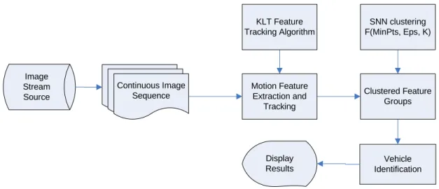
The KLT motion feature based tracking approach implemented in this project is illustrated in Figure 3-1. The algorithm consists of two major components, the KLT feature tracking module and the Shared Nearest Neighbor (SNN) clustering module, explained in detail in the following sections.
Image Stream Source Vehicle Identification Continuous Image Sequence Display Results Motion Feature Extraction and Tracking Clustered Feature Groups KLT Feature Tracking Algorithm SNN clustering F(MinPts, Eps, K)
Figure 3-1: Proposed KLT-SNN approach.
3.1.1 KLT Feature Tracking
A KLT motion-feature-based algorithm for detection and tracking is first attempted. Video sequences can be treated simply as sequences of images. Good KLT
motion features can be located by examining the minimum eigenvalue of each 2 by 2 gradient matrix. A particular feature point with coordinates (x, y) on the image frame captured at time t can be mathematically described as I(x ,y ,t). KLT feature tracking can be accomplished by examining two consecutive video frames t and t+1 and finding the matching point on image frame t+1 for the feature point on image frame t. Feature point movements between consecutive image frames are constrained by vehicle speed, camera settings, and roadway geometrics. Therefore, a feature point’s position can be predicted to fall in a pixel window W on next image frame. To locate the exact location of the feature point (x, y) on next image frame, the displacement parameters Δx,Δy that minimize the sum of squared intensity differences of points in W, ε, between frames t and t+1 must be computed (Bouguet, 1999):
[
]
2( x, y) W I x y t( , , ) I x( x y, y t, 1
ε Δ Δ =
∑∑
− + Δ + Δ + (3-1)The Newton-Raphson search method can be used to find Δx,Δy. Once the displacement parameters are known, feature points can be tracked from frame to frame. It is important to select salient features to track. The selection is based on the following procedure suggested by Bouguet (1999):
1. Compute the gradient (G) matrix and its minimum eigenvalue λmat every pixel in the image.
2. Call λmax the maximum value of λm over the whole image.
3. Retain the image pixels that have a λm value larger than 5-10% percent of
max λ .
4. From those pixels, retain the local maxima pixels (a pixel is kept if its λm value is larger than that of any other pixel in its window W).
5. Keep the subset of those pixels so that the minimum distance between any pair of pixels is larger than a given threshold distance.
The G matrix is defined as follows:
∑∑
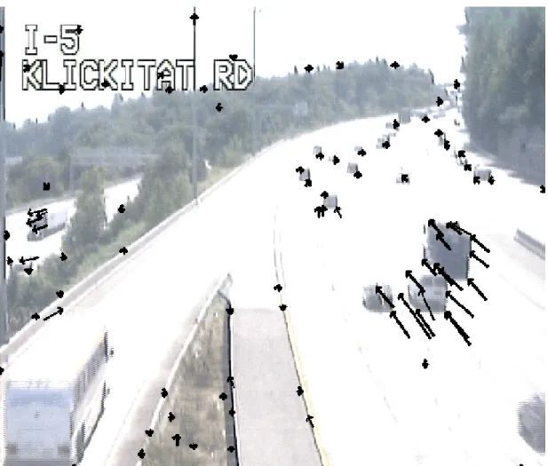
⎥⎥ ⎦ ⎤ ⎢ ⎢ ⎣ ⎡ = W y y x y x x t y x I t y x I t y x I t y x I t y x I t y x I G ) , , ( ) , , ( ) , , ( ) , , ( ) , , ( ) , , ( 2 2 (3-2)The window W was specified at 3 x 3 pixels to reduce computational complexity. Figure 3-2 shows the resulting displacement vectors in a test sequence. Once the features are selected and tracked, a clustering algorithm is necessary to group features belonging to the same object together.
3.1.2 SNN Clustering
Feature point clustering is an important step for video-based vehicle detection and tracking. The K-means algorithm is a popular approach for point clustering and was naturally considered for this study. Additionally, several other clustering algorithms needed to be examined to identify the best clustering approach. The KLT feature points extracted using the method proposed by Tomasi and Kanade (1991) and Shi and Tomasi (1994) tend to form clusters of different densities. This is due to the perspective effect, i.e. when nearby vehicles move further away from the camera, the distances between feature points decrease, increasing the density and decreasing the size of the potential cluster of feature points. This posed a potential issue for the K-means clustering, which cannot deal with clusters of varying density and size (Ertoz et al., 2003). Furthermore, K-means clustering is often sensitive to outliers and produces unfavorable results when image noise present. Therefore, this study investigated several other clustering algorithms and the SNN clustering algorithm was selected as a superior alternative because it is robust to noise and handles clusters of varying density and size.
Unlike the K-means algorithm, SNN clustering is based on the principle of common nearest neighbors and does not need prior knowledge of the number of clusters. The SNN algorithm contains eight steps (Ertoz et al., 2003):
1. Compute the similarity matrix. (This corresponds to a similarity graph with data points for nodes and edges whose weights are the similarities between data points.)
2. Sparsify the similarity matrix by keeping only the k most similar neighbors. 3. Construct the shared nearest neighbor graph from the sparsified similarity
4. For every node (data point) in the graph, calculate the total strength of links coming out of the point.
5. Identify representative points by choosing the points that have high density, i.e., high total link strength.
6. Identify noise points by choosing the points that have low density (total link strength) and remove them.
7. Remove all links between points that have weight smaller than a threshold. 8. Take connected components of points to form clusters, where every point in a cluster is either a representative point or is connected to a representative point.
This procedure can be completed in real time even when used in conjunction with KLT feature tracking.
3.1.3 Initial Test Results
The proposed KLT-SNN approach was initially tested in several simple scenarios, such as free-flow freeway scenes. Through this initial experiment, the key difficulty of the proposed KLT-SNN approach is found to be the ability to assign the tracked feature points to their context-appropriate groups. The SNN algorithm is meant to group feature points based on velocity and position to form groups, each representing a vehicle.
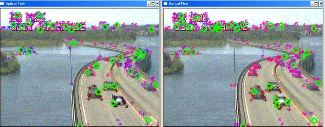
Figure 3-3 shows four consecutive frame examples when the KLT-SNN approach is applied. The arrows on the frames represent the vectors resulting from the KLT algorithm and the green circles are the cluster centers found by the SSN algorithm. It can be seen that the number and location of the obtained clusters varies significantly from frame to frame, indicating the difficulty in using the KLT-SNN method to count vehicles accurately. The KLT-SNN approach faced three major challenges. First, several clusters are often assigned to a single vehicle, considerably reducing accuracy. Second, noise
turned out to be a significant issue, despite the use filtering techniques. Noise features were so dominant that many clusters are formed entirely of noise, despite attempts at filtering by velocity. A noise cluster can be seen bottom-right corner of all the frames in Figure 3-3. Finally, occlusion reasoning was difficult to perform due to the number of extraneous clusters. Because a vehicle could be represented by several clusters, it would be difficult to reason where one vehicle ends and another begins.
Additional measures were necessary to improve results. Although further filtering can improve the KLT-SNN results, the potential is limited. Therefore, a different algorithm was sought to supplement the existing approach.
Figure 3-3: KLT-SNN initial test results.
3.2
Scan-line Based Approach
3.2.1 Approach Concept
As shown in Section 3.1.3 Initial Test Result, the KLT-SNN approach had difficulties in detecting vehicles, especially when the partially occluded vehicles are moving at the same speed because “motion” is the main feature for clustering. Therefore, in order to improve KLT-SNN detection and tracking, a supplementary approach was
a) Frame 1: 41 Clusters b) Frame 2: 32 Clusters
needed to mitigate certain clustering issues and assist with occlusion reasoning. Additional detection algorithms can reinforce the hypothesis generated through KLT-SNN and thus enhance accuracy. On the other hand, implementing two algorithms concurrently may degrade the computing efficiency and detection capability of the existing algorithm.
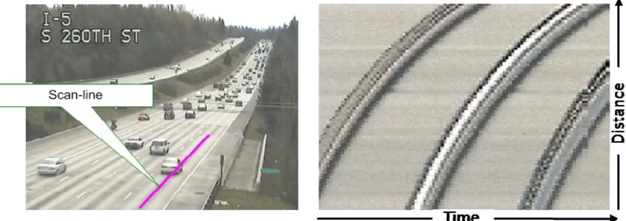
Herein, a scan-line based approach is proposed to provide an additional cue. This cue should be invariant to environmental factors and could be used for occlusion reasoning. Placing a scan-line along the direction of movement of the vehicles can be helpful to identify regions where vehicles are present. As mentioned in Section 2.1.7, a traditional scan-line approach can detect vehicles by comparing the present state to a background, or by examining the vehicle edges found along the line. In this research, an additional dimension, time, is added to the traditional scan-line approach. Figure 3-4 displays the result of composing multiple snapshots of the pixels present on the scan-line in Figure 3-4 (a) into a time-space image hereafter referred to as a Spatial-Temporal (ST) map, displayed in Figure 3-4 (b). In other words, all the pixel intensities on the scan-line will be recorded at every frame and shown progressively line by line on the ST-Map (Figure 3-4(b)).
(a) Scan-Line (b) Corresponding ST-map Figure 3-4: ST-Map Example (Malinovskiy et. al, 2008).
The strands that appear in the ST-map represent the approximate trajectory of the vehicles in the lane. Analyzing this simple image would generate the necessary information regarding vehicle movement in that lane. In the following sections, the proposed ST-map approach will be explained.
3.2.2 ST-Map Algorithm Overview
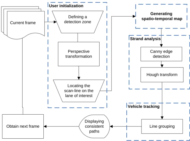
Figure 3-5 displays the flow chart of the ST-map algorithm. The algorithm consists of four primary logical steps, which are boxed in dashed lines on Figure 3-5.
Generating spatio-temporal map Canny edge detection Hough transform Displaying consistent paths Obtain next frame
User initialization Defining a detection zone Perspective transformation Line grouping Locating the scan-line on the lane of interest Strand analysis Current frame Vehicle tracking
Figure 3-5: Flow chart of the ST-map algorithm (Malinovskiy et al., 2008).
The initial step for the ST-map algorithm is user initialization. This step is performed once. This involves having the user draw a rectangle in the scene to determine the detection zone and obtain homography parameters. After the homography parameters are determined, the transformed images can be generated continuously. The user is free to place up to 20 scan-lines on the transformed image. Following initialization, the ST-map can be generated for each of the placed scan-lines in the second step. Strand analysis is performed in the third step. In this step, the Canny (Canny, 1986) edge filter is used and then the Hough transform (Hough, 1959; Gonzales, 2000) is performed to obtain lines characterizing the strands present in the ST-map. The last step is to group these Hough lines to separate different vehicles. Once these Hough lines are obtained, a
connected-The graph is then searched for connected components; each connected component represents a potential vehicle. This step is also called vehicle tracking. In the proposed approach, vehicle tracking and detection are finished in the same procedure. The details will be elaborated.
3.2.3 User Initialization
User initialization is the first step of the proposed algorithm. As shown in Figure 3-4, the strands in the ST-maps obtained using a scan-line are spatially distorted from the true trajectories of the vehicles due to perspective because pixels farther away from the camera represent greater actual distance in the scene shown in Figure 3-4(a). Typically vehicles travel at nearly a constant speed over a short distance under unconstrained conditions. This should result in nearly linear trajectories in the world coordinates rather than the curved ones shown in Figure 3-4(b).
In order to correct this distortion error, a perspective image transformation should be performed. This procedure can transform scene images to a top-view images (from image coordinates to world coordinates). Normally, it is performed through the homography matrix Hab. Acquiring this matrix requires knowledge of scene points as
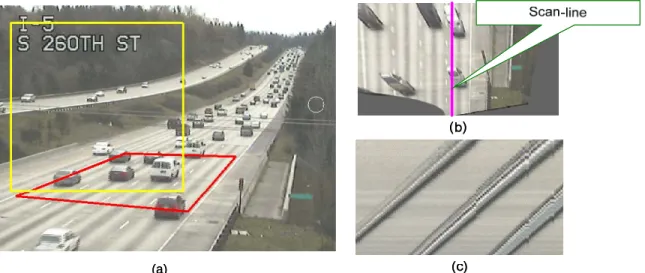
well as camera parameters. Such information can be easily obtained by a manual user initialization procedure proposed in this study. In this procedure, a user is required to specify a detection zone by selecting four points on the road surface that would represent a square in the scene, as shown by the red quadrangle in Figure 3-6(a). This quadrangle must have a side perpendicular to the movement of the vehicles. Then, this quadrangle is rectified into a pixel-coordinate square, as demonstrated by the yellow square in Figure
3-specified quadrangle and is used to compute the homography matrix. After the transformation through the homography matrix is performed, the perspective distortion can be corrected, as shown in Figure 3-6(b). Once the perspective transformation is complete, the ST-map can be generated, as shown in Figure 3-6(c).
Note that the perspective transform performed for the algorithm is accurate in a specific 2D plan only. This means the points that are not on the ground plane are still distorted. This is evident by the increased height distortion of vehicles observable in Figure 3-6(b) as they move away from the camera.
(a) (a)
Figure 3-6: User initialization: (a) defining a detection zone, (b) user defined detection zone after perspective transformation, and (c) ST map retrieved from a scan-line (Malinovskiy et al., 2008).
As previously mentioned, the transformation matrix Hab is required to perform the
perspective transform. Finding Hab requires two four-point sets: the four user-input points
(corner points of the red quadrangle) that corresponds to a perfect square in the real world and the four corner points of the yellow square automatically constructed using the
coordinates in the actual scene, while the automatically constructed points are considered to be their pixel-coordinate mappings. Actually, we may not know four points in the scene that are corner points of a square. However, this does not matter much for vehicle detection. As long as we can identify four points that are corner points of a rectangle in the scene, the remaining distortion only affects the ratio of vehicle length to width. If this scan-line approach is used for vehicle speed measurement, then the four points must be corner points of a square.
Solving for Hab allows one to compute the pixel mapping of any other points in
the real scene and thus render the scene in a top-view perspective. As shown in Equation 3-3, Ηabis a 3x3 matrix containing six unknowns:
11 12 13 21 22 23
0
0
1
abh
h
h
h
h
h
⎡
⎤
⎢
⎥
Η = ⎢
⎥
⎢
⎥
⎣
⎦
(3-3)Suppose point pa in pixel coordinates can be represented as pa =
[
xa ya 1 ']
and its corresponding mapping point pb in the real-world scene is represented as[
1 ']
b b b
p = x y . Ηab can then be computed using four matching point sets and the
relationship:
p
b= Η
abp
a. With Ηabknown, the relationship between the scene and 2D image plan can be found, and the top-view image can be formed. The distortion-free ST-maps can be constructed by placing a scan line on the top-view image.3.2.4 Strand Analysis
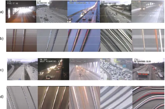
Figure 3-7 displays a variety of environments shown in rows a) and c) and the corresponding ST-Maps from the above environments are displayed in rows b) and d). The advantages of the ST-map cue are immediately apparent. The resulting strands not only give convenient vehicle trajectories that are significantly simpler to analyze, but are also remarkably identical regardless of environmental conditions. These strands are presented on a relatively uniform background. All ST-maps consist of linear strands extending from the top to the bottom of the map. An exception to this rule can be seen in the right-most image of row (d) of Figure 3-7. This image shows that traffic has varying speed over the scan-line, thus creating non-linear strands. However, all other scenarios possess identical near-linear trajectory characteristics and the detection. The proposed vehicle tracking algorithm focuses on detecting vehicles by analyzing the linear strands.
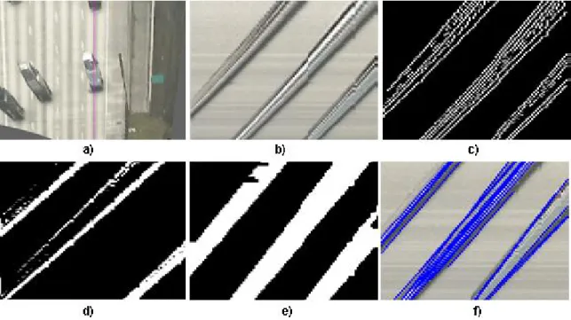
The key to successful vehicle tracking now becomes segmenting the strands from the ST-map. This can be done in several ways, simplest of which is by using background subtraction techniques as discussed in Section 2.1.2. Figure 3-8 shows the preprocessing steps necessary for segmentation in Figures 3-8 (a,b,c) and the resulting segmentations in Figures 3-8 (d,e,f). Since the background is constantly updating and is uniform enough, it is possible to maintain a vector of background pixel values. The incoming scan-line values can then be compared against this mode background vector and labeled as either background or foreground pixels. The result of such an approach can be seen in Figure 3-8(d), showing segmented strands from Figure 3-8(b) which were obtained from the scene shown in Figure 3-8(a). The segmentation obtained is fractured due to the likeness of the similarity of vehicle pixels and pavement pixels. Although there were originally three strands, indicating three vehicles have passed within that lane, the result from the background subtraction produces four strands, resulting in an over-count.
Another potential approach is edge dilation. Figure 3-8(c) shows the result of running a Canny edge detection (Canny, 1986) algorithm on the strands. Using a dilation operation on such an image, the segmentation shown in Figure 3-8(e) can be obtained. Details about the dilation algorithm can be found in (Shapiro and Stockman, 2001). This results is a significant improvement over background subtraction. As shown in 3-8(e), three vehicles are successfully segmented but if these vehicles are very close, the dilated strands will be merged and regarded as one vehicle.
As a result, a third approach is developed in this research to deal with such occlusion issues. Figure 3-8(f) shows the result of performing a Hough transform
(Hough, 1959; Gonzales, 2000) on the Canny edge image in Figure 3-8(c). The blue lines represent the Hough lines detected and produced by the Hough transform algorithm.
Figure 3-8: Strand analysis via various strand segmentation techniques.
As shown in Figure 3-9, these Hough lines will converge to a theoretical convergence point. If this point can be determined, these strands intersected at the same convergence point can be regarded as a group (a vehicle). The convergence is formed due to the height distortion introduced by the perspective transformation. As a vehicle moves farther away from the camera it appears taller and taller due to perspective distortion, as only the ground plane is accurately transformed in a two-dimensional perspective change. This distortion plays an important role in strand segmentation (line grouping). As the vehicle moves further away, the strand the vehicle leaves becomes thicker and the extensions of the Hough lines that are obtained from the strand begin to converge below the image.
Therefore, by determining the groups of convergence, one can determine the number of vehicles passing the detection zone. For example, one can also easily conclude that there are three vehicles shown in Figure 3-9. Unfortunately, the convergence groups are not easy to determine in practice because image noise and camera vibrations will cause the Hough lines to have slightly varying trajectories, thus resulting in several convergence points. Hence, Hough line grouping becomes more challenging in practice.
Figure 3-9: Theoretical convergence of the Hough lines (Malinovskiy, et al., 2008). 3.2.5 Hough Line Grouping
at the same convergence point. This issue is illustrated in a simplified example in Figure 3-10(a). The dashed rectangle represents the viewable ST-map on the screen to be analyzed, while the red and blue lines are the Hough lines from two different groups of strands produced by two different vehicles. Multiple intersection points can be seen. It is possible to group the lines by clustering these intersections because proximal intersections should belong to the same strand group. However, such a solution has proved infeasible by providing inconsistent results due to the constantly changing cluster sizes and variable intersection densities.
As a result, the concept of “first intersection” is introduced. This intersection is the first intersection where a given Hough line intersects with the proximal Hough line below the bottom of the ST-map. These first intersections are illustrated as green dots in Figure 3-10(a). This is meant to represent the intersection that appears near the theoretical convergence point. The Hough line may intersect with many other Hough lines above and below the first intersection, but those intersections are ignored.
Clustering these first-intersections becomes critical. In the research, connected component concept is adopted to cluster these first-intersections. As shown in Figure 3-10(b), each Hough line represents a node and each first-intersection pair represents an edge between the nodes. A first-intersection pair is determined by the relationship that two lines first intersect. For example, in Figure 3-10(a), Line 7 first intersects line 6, and there is an edge connecting their nodes in the graph. Lines 5 and 7 are also connected by an edge, as line 5 first intersect line 7. The first intersection relationships of lines 5, 6 and 7 are plotted as a non-directional graph in the lower part of Figure 3-10(b). Now it can be seen that lines 5, 6 and 7 form a completely isolated and independent graph from the
group of lines 1, 2, 3 and 4. Thus, two different groups of strands can be determined and regarded as two vehicles.
2 1 3 4 5 6 7 (a) (b)
Figure 3-10: Demonstration of line grouping for vehicle detection: (a) Hough lines, and (b) result of the constructed graphs (Malinovskiy, et al., 2008).
Tarjan’s strongly connected components algorithm (Tarjan, 1972) is used to determine the connected components of the graph created by the first intersection pairs. BOOST C++ libraries are used in this algorithm to construct first-intersection graphs and determine the connected components (BOOST, 2008). The obtained connected components represent vehicles. Each connected components consists of several Hough lines, and the average slope these Hough lines is the trajectory of the vehicle. This allows for retrieval of the complete spatio-temporal history of the vehicle during its progression through the detections zone.
3.2.6 Preliminary Results and Conclusions
Based on our preliminary tests, the scan-line based algorithm developed in this study significantly outperformed the KLT-SNN algorithm in both adverse environment and occluded conditions. For real-time applications, the scan-line-based algorithm was also found to be more suitable because it consumes less computing resources than the KLT-SNN algorithm. Although the KLT-SNN algorithm has its advantage in some cases, combining the scan-line-based algorithm and the KLT-SNN algorithm increases the computational complexity and degrades the efficiency. Thus, the scan-line based algorithm was chosen for further development and improvement, without the use of the KLT-SNN algorithm.
4
E
XPERIMENTS AND
R
ESULTS
4.1
Experimental Setup
4.1.1 Software Development Environment and Required Hardware
In order to develop a real-time vehicle detection and tracking system, the ST-map algorithm was implemented in the C++ computer language. C++ offers direct memory management and does not have the external garbage collection costs associated with some higher level languages such as Java and C#. C++ also offers valuable libraries for computer vision and video processing as well as graph building and searching. A C++ console application was built with minimum functions to maximize performance.
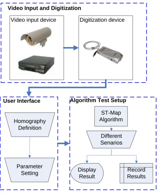
The ST-map algorithm was tested using the hardware configuration shown in Figure 4-1. Video data can be obtained from live or taped surveillance footage and sent to the computer through a TV-tuner card. Once the information is digitized, user input is necessary to initiate the perspective transform and determine basic parameters. The video-based vehicle detection system can then begin to analyze the input video sequence. Details of the experiments are described in the following sections.
Digitization device Video input device
ST-Map Algorithm Homography Definition Display Result Record Results Parameter Setting
User Interface Algorithm Test Setup
Video Input and Digitization
Different Senarios
Figure 4-1: Test setup.
4.1.2 Video Input and Digitalization
The ST-map algorithm implementation was tested on a Sony Vaio SZ-110 Laptop running Windows XP on a 1.8Ghz Intel Core Duo processor, 2 GB of RAM and a GeForce Go 7400 video adapter. This is representative of an average portable computer system in use today. Since the ST-map algorithm was developed with surveillance camera deployment in mind, it was tested under similar conditions. A DirectX module
external video devices. The module automatically detects any external video inputs and selects one to process. During testing, a digital TV-tuner card, WinTV for this study, was used to translate analog video into a digital signal, fed to the mobile computer through the USB port.
The ST-map algorithm test setup does not differentiate between live video coming from one of the many WSDOT camera installations or video coming from a tape being played on a VCR player. For the purposes of testing, taped scenarios were used in order to be able to be able to repeat the testing sequences when further adjustments to the algorithm were deemed necessary. Although any input resolution can be chosen through the DirectX input module, a consistent value of 320 x 240 was chosen to ensure real-time performance. Higher resolution video inputs may generate better results, but are currently too computation intensive for consistent real-time performance on our computer system.
4.1.3 User Interface
A simple and low-overhead user interface system was designed for the ST-map algorithm. To begin vehicle analysis, a user must perform a few simple tasks upon running the executable. When the algorithm initiates, a window titled “Input Video” is displayed and the input video is shown, as illustrated in Figure 4-2.
Figure 4-2: Input video display window.
Upon confirming that the desired video input has been selected, the user must now define the four points that are necessary for solving the homography matrix. This is done by pressing key “D” on the keyboard to activate the definition window, titled “Homography Definition”. On the definition window, the user must draw four points that represent a square in the scene by using the right mouse button to specify the point locations in a counter-clockwise order. An example of the homography defining procedure is illustrated in Figure 4-3, where the first and second segments have been
perpendicular to the direction of movement of the vehicles. The size and location of the square should be roughly the desired detection zone.
Figure 4-3: Homography definition.
Once the four necessary homography points have been defined, a new screen-coordinate square is generated in the Homography Definition window, as shown in Figure 3-6(a). As mentioned earlier, the four corner points of the newly generated square show the remaining four points needed for the transformation. At this point, the Homography Definition window can be closed. It should be noted that the window may
Once the perspective transform is complete, the user defines some basic parameters. Parameters are defined by moving sliders on the track-bars in the “Parameter Definition” window summoned by pressing “P” on the keyboard. Figure 4-4 shows an example Parameter Definition window. There are six track-bars in the window. The “Canny 1” track-bar adjusts the upper threshold of the Canny algorithm, while the “Canny 2” track-bar adjusts the lower threshold of the Canny algorithm. The default parameters specified are 120 for Canny 1 and 100 for Canny 2. We have found these parameters applicable in most situations; however the user is free to modify these settings. It is required to keep the Canny 1 value higher than Canny 2, as it is the upper threshold.
The “Hough” track-bar adjusts the threshold of the Hough transform, lower values will produce more Hough lines. Additional Hough lines assist detection quality, but consume a significant amount of computing resources, thus this value is best set in accordance with the performance of the user’s machine.
The “Length” track-bar is responsible for setting the minimum length of vehicle in pixels. This value helps filter out potential noise and is dependent on the camera angle. During testing, this value varied between 50 and 100 pixels, depending on the position of the detection zone and proximity of vehicles to the camera.
(b)
(a) (c)
Figure 4-4: Interface windows (a) parameter definition window, (b) ST-map window, and (c) Canny edge window.
The “Scan-Line” track-bar moves the current inactive scan-line horizontally. To activate a scan-line in the position currently dictated by the Scan-Line track-bar, the user must press “L” on the keyboard. This locks the current scan-line into scanning that position and creates ST-maps based on that input. The track-bar slider may then be
line. This can be repeated as often as needed, but it should be noted that additional active scan-lines generate additional ST-maps and therefore consume significant computational resources. Once the desired scan-lines are active, the algorithm may proceed to automatically number and mark detected vehicles, as illustrated in Figure 4-4(a). The numbering system counts the amount of vehicles per individual scan-line.
The effects of the first three sliders in the Parameter Definition window can only be seen if the user looks at the generated ST-maps and their resulting edges and Hough lines. This can be done by pressing “X” on the keyboard. Two windows will pop up, one displaying the ST-map generated for the last activated scan-line, titled “ST-map” (see Figure 4-4(b) and the other, titled “Canny Edges” (see Figure 4-4(c)) will display the result of running the Canny algorithm on that ST-map. The Hough lines obtained from the Canny edges will be displayed as superimposed on the ST-map shown in the “ST-map” window. Based on these windows, the user can adjust the sliders to produce contiguous edges and the maximum number of Hough lines that can be handled in real time by the user’s machine.
Although the controls are not intuitive, they provide the quickest and computationally inexpensive means of interacting with the algorithm test setup. Table 4-1 summarizes the keys necessary for operation.
Table 4-1: Key mappings
Summon Key Effect
"D" Homography Definition Window "P" Parameter Definition Window "L" Activate Scan-line "X" ST-map and Edges Windows
4.1.4 Algorithm Test Setup
The proposed ST-map algorithm was tested using five hour-long sequences featuring a range of environmental issues to ensure stability and adequate performance. Additionally, the algorithm was also tested and examined frame-by-frame using three 10-minute video segments to demonstrate common errors and limitations. Testing was done using two scan-lines for consistent comparisons. The results, such as time stamps, vehicle positions and vehicle labels for each lane, were recorded in a text file.
4.2
Experimental Results
4.2.1 Stability and Overall Performance Experiments
Stability and overall performance testing was performed using five SR-520 surveillance video sequences taken at the east entrance of the Evergreen Point Floating Bridge in Washington State (hereafter, called SR-520 East). The five sequences were taken at an identical location to compare the impacts of adverse weather conditions, as well as the effect of traffic volumes on accuracy a screenshot of the tested location is shown in Figure 4-5.
Figure 4-5:SR-520 East testing site.
Figure 4-6 shows the snapshots of the beginning, middle, and end of the first sequence of SR-520. This sequence was taken from 8:30 pm to 9:30 pm on June 4, 2008. The sequence suffers from drastic ambient light changes as well as some camera vibration issues.
Figure 4-6: The snapshots of the first sequence of SR-520 East during 8:30 pm – 9:30 pm on June 4, 2008.
Table 4-2 presents the overall error result for both lanes of the first sequence. An error rate is adopted as an index to evaluate the algorithm performance and is defined as: (ground truth count – detected count)/(ground truth count) x 100%
The counting error rate is fairly low for left and right lane, -1.3% and 1.0%, respectively. This result shows the proposed algorithm is robust enough to handle lighting variations. Furthermore, the performance is not significantly affected by headlight reflections on the pavement when the scene is dim.
Table 4-2: The result of 8:30 pm – 9:30 pm, June 4, 2008
Performance measure Left lane Right lane
Manual count 871 841
ST-map 882 833
Error rate -1.3% 1.0%
Figure 4-7 shows the snapshots of the second sequence on SR-520, recorded from 8:30 pm to 9:30 pm, on October 27, 2008. This scene is much more challenging than the first sequence since the scene is totally obscure except the lights from vehicle headlights. Hence, this nighttime sequence contains severe headlight reflections and glare, as well as a general reduction of visibility.
Figure 4-7: The snapshots of the second sequence of SR-520 East, 8:30 pm – 9:30 pm, October 27, 2008.
Table 4-3 presents the overall error result for both lanes of the second sequence. These results show that the algorithm performance degraded because the difficulties caused by the lighting issues, but the error rate was within 10%. The left lane’s higher error rate can be attributed to the glare of oncoming vehicles. The glare obscured some portions of the vehicle’s trajectory.
Table 4-3: The result of 8:30 pm – 9:30 pm, October 27, 2008
Performance measure Left lane Right lane
Manual count 760 822
ST-map count 687 827
Error rate 9.61% -0.61%
Figure 4-8 shows the snapshots from the third sequence. This sequence was significantly more challenging due to the presence of water-trails, wet pavement glare, and strong wind-induced vibrations. The sequence also contained a significantly higher vehicle volume and created numerous occlusions, as can be seen in the right-most frame of Figure 4-8.
Figure 4-8: The snapshots of the third sequence of SR-520 East 11:30 am – 12:30 pm on June 4, 2008.
The results achieved were promising considering the amount of factors at play. Table 4-4 shows the results for the third sequence. The left lane has the higher error rate then the right lane. This may be because the higher traffic volume results in higher chances of occlusions.
Table 4-4: The result of 11:30 pm – 12:30 pm, June 4, 2008
Performance measure Left lane Right lane
Manual count 1556 1302
ST-map count 1328 1194
Error rate 14.7% 8.3%
Snapshots of the fourth sequence can be seen in Figure 4-9. This sequence was taken during 12 pm – 1 pm on October 27, 2008 and contains a sunny-day situation, with moderate shadows, camera shake and nearly constant ambient lighting conditions.
Figure 4-9: The snapshots of the fourth sequence of SR-520 East 12:00 pm – 1:00 pm on October, 27, 2008.
Results for the fourth sequence are given in Table 4-5. The left lane has relatively lower accuracy than the right. This may be attributed to a higher percentage of occlusions, as the lane was blocked by vehicles travelling in the right lane.
Manual count 1554 1296
ST-map count 1348 1239
Error rate 13.26% 4.40%
The snapshots of the last SR-520 sequence are shown in Figure 4-10. This scene suffered primarily from long shadows, moderate vibrations and high volumes, due to rush hour traffic from 4:30 pm to 5:30 pm on October 27, 2008.
Figure 4-10: The snapshots of the fifth sequence of SR-520 East 4:30 pm – 5:30 pm on October, 27, 2008.
High volumes in the scene caused numerous occlusions, such as the one seen in the middle frame of Figure 4-10. Table 4-6 shows the result of running the ST-map algorithm on the above se