Composing Supply Chains through Multi-unit
Combinatorial Reverse Auctions with
Transformability Relationships among Goods
Andrea Giovannucci, Jes ´us Cerquides, and Juan A. Rodr´ıguez-Aguilar
Abstract—In this paper we provide a decision support system (DSS) to auctioneers when assembling their supply chains. Some-times an auctioneer/buyer has to decide whether to outsource some production processes or not (make-or-buy decision). For this purpose we add a new dimension to the goods at auction. A buyer can express transformability relationships (t-relationships) among goods: some goods can be transformed into others at some transformation cost. On the other hand, often another type of relationship among the goods at auction exists on the bidders’ side, that is complementarity relationships. Combinato-rial auctions are usually employed to deal with the problem of complementarities on the bidders’ side. Then, in this paper we build upon combinatorial auctions to implement a DSS to solve make-or-buy decisions in markets characterized by combinatorial preferences.
Firstly, we introduce the information about transformability relationships in the combinatorial auctions winner determination problem (WDP) so that an auctioneer/buyer can assess what goods to buy, to whom, and what transformations to apply to the acquired goods in order to obtain the required ones. In this way, an auctioneer can build his supply chain maximizing his revenue. We call the resulting model Multi-Unit Combinatorial Reverse Auction with Transformability Relationships Among Goods (MUCRAtR). This new auction type allows a buyer/auctioneer to express and communicate to bidders its internal production structure and its final requirements. Bidders can then formulate appropriate offers and send them back to the auctioneer. Upon receiving the offers, an auctioneer can determine, by means of a public selection rule, the cost minimizing combination of bids along with the internal operations leading to its final require-ments. In order to solve the Winner Determination Problem. we map it to an optimization problem on Place/Transition Nets. Such mapping allows to efficiently solve the WDP for some problem classes, and provides a set of powerful formal tools for describing the underlying optimization problem. Finally, we quantitatively assess the potential benefits and drawbacks when considering transformability relationships.
Index Terms—Supply Chain, Combinatorial Auctions, Winner Determination Problem, Petri nets
I. INTRODUCTION
A. Motivations
We are witnessing an important transformation of the firm organizational structure. Today’s business world is experi-encing a progressive disintegration of the traditional vertical
Andrea Giovannucci and Juan A. Rodr´ıguez-Aguilar are with the Artificial Intelligence Research Institute, Spanish National Research Council, Bellaterra, Barcelona, 08193 SPAIN e-mail:{andrea,jar}@iiia.csic.es.
Jes ´us Cerquides is with the University of Barcelona. Gran Via de les Corts Catalanes, 585, 08007 Barcelona. Spain.
integrity1 of the enterprises’ organizational structure. This is witnessed by a heavy increment in the use of outsourcing. In-deed, the structural integrity of organizations is breaking down; the traditional vertically integrated organizations, controlling as many of the production factors as possible, is being quickly replaced by better focused and more specialized organizations. An increased number of capable service providers, the pressure deriving from the hypercompetitivity, and the pervasive pres-ence of technology impose a new strategic vision. As a result, new supply chain management [60] strategies are emerging, like strategic outsourcing [54], [31], [18] and collaborative supply chain network design [63]. This situation requires an increased automation across the supply chain. Indeed, static and vertically integrated supply chains are quickly giving way to more flexible value chains composed of partners that can be assembled in real time to meet unique requirements.
In this environment, it is critical the rapid, automatic and reliable selection of the right business partners. As a revealing phenomenon, one of the main objectives of current supply chain management [60] is to integrate as much as possible the
back-end of the supply chain (its production and
manufactur-ing portion) to the front-end (the final customer).
A spectrum of possible solutions is possibly needed by en-terprises. On the one extreme, companies must make decisions about whether to outsource part of their production processes (buy/make decisions) in business environments characterized by myriads of possible partners (lower barriers caused an in-crement in competition). On the other extreme of the spectrum, virtual enterprises may need agile decision support systems (DSSs) that allow them to automatically form self-organizing supply chains. Indeed, we do believe that nowadays firms require DSSs that allow them to nimbly and automatically select strategic business partners. As a first step, those DSSs should allow firms to automate the process of partner selection, optimizing critical make-or-buy decisions across the supply chain (i.e. trading off decisions of internal vs external pro-duction) with multiple potential partners. With this aim, we deem absolutely necessary to tightly integrate the procurement and outsourcing strategies and decisions. Thus, the decision support should allow them to self-organize by allowing to:
• integrate and coordinate all the supply chain stake hold-ers;
1In microeconomics and management the term vertical integration describes
the degree to which a firm owns its upstream suppliers and its downstream buyers.
• include component suppliers into the supply chain design process;
• optimize the overall performance of the supply chain (i.e. not a local optimization);
• negotiate based on direct cost competition, that trades off decisions of internal vs external production. It is well known that one of the positive results of outsourcing is putting in competition the internal activities of an enterprise with the outside world.
• to express the partners’ preferences in a flexible and efficient way.
With the above-mentioned requirements fulfilled, competitive companies could easily cope with the selection of optimal, tightly connected procurement, outsourcing, and collaboration strategies.
B. Requirements
In what follows we present a motivating example concerning the main issue we intend to face in this thesis: the problem of efficiently solving make-or-buy decisions across the supply chain when complementarities among goods hold on the bidders’ side.
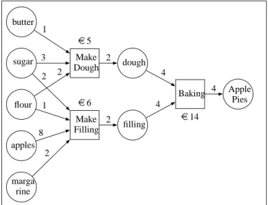
Example I.1. Consider a company, named Grandma & co,
devoted to produce and sell apple pies. The internal produc-tion structure of the company, i.e. the way apple pies are prepared, is presented in figure 1. Each circle represents a raw, intermediate or manufactured good. Squares connecting goods represent manufacturing operations. An arc connecting a good to an operation indicates that the good is an input to the operation, whereas an arc connecting an operation to a good indicates that the good is an output of the operation. Then, butter, sugar, and flour are input goods to the Make
Dough operation, whereas dough is an output good of the Make Dough operation. The labels on the arcs connecting input goods to operations, and the labels on the arcs connecting output goods to operations indicate the units required of each input good to perform an operation and the units generated
per output good respectively. In our example, the preparation of two units of dough requires one unit of butter, three units of sugar, and two units of flour.
Each operation has an associated cost every time it is carried out. We label each operation with a cost. In our example, the
Make Dough operation costs 5 e.
Consider that the marketing department at Grandma & co forecasts that two hundred apple pies will be sold within a month and that the stock of Grandma & co is composed of one hundred units of flour and two hundreds units of sugar. Therefore, the company starts an automated sourcing [32] process to acquire the basic ingredients needed for producing pies, namely butter, sugar, flour, apples, and margarine.
However, the production management staff decides to test a new sourcing process. Instead of limiting the procurement to basic ingredients, they decide to incorporate in the sourcing process intermediate and final goods as well, namely dough,
filling, and apple pies in figure 1. More precisely, the
pro-duction management wonders whether to outsource part of its production process. In fact, the executive staff noticed that
butter sugar flour apples marga rine Make Dough e5 Make Filling e6 1 3 2 2 1 8 2 dough filling 2 2 Baking e14 4 4 Apple Pies 4
Fig. 1. Apple pie production flow.
more and more specialized enterprises are entering the organic food market. Since Grandma & co is a well-known brand for pies, it decides that in order to reduce costs, it could be suitable to negotiate and collaborate with those new brands.
As an additional constraint, the production management knows that strong complementarities among the negotiated goods exist on the supplier side. For instance, suppliers often sell margarine and butter as indivisible bundles. Thus, it is required that those complementarities are taken into account.
Grandma & co realizes that it faces a decision problem:
shall it buy the required ingredients and internally produce apple pies, or buy already-made apple pies (outsource all its production), or opt for a mixed purchase and buy some ingredients for internal production and some already-made apple pies? This concern is reasonable since the cost of ingredients plus preparation costs may eventually be higher than the cost of already-made apple pies. Grandma & co must take a decision among many possible mutually exclusive options:
• buy all the basic ingredients to internally produce all the pies;
• buy from suppliers all the pies and resell them under its name;
• buy already-made dough and filling from suppliers , and bake itself the cake;
• prepare part of the dough and part of the filling, and buy the rest from suppliers;
• buy part of the pies from suppliers and produce the rest itself;
Grandma & co is interested in quantitatively assessing what
to buy and from whom, as well as what to produce in house. Such assessment depends on many factors:
(1) the market cost of the basic ingredients (butter, sugar, flour, apples, and margarine);
(2) the market cost of dough, filling, and pies; (3) the stock goods at Grandma & co;
(4) the finally required goods (the sales forecast);
(5) the cost for performing at Grandma & co the operations
Make Dough, Make Filling, and Baking (the internal cost
structure);
(6) the number of units of each good either produced or required for each operation (the internal production structure); and
(7) the complementarity relationships among goods holding on the suppliers’ side.
Hence, Grandma & co requires a complex decision support system along with a negotiation mechanism that helps it in detecting which is the revenue maximizing buying config-uration and the internal operations to perform in order to obtain the finally required goods. It is easy to understand from the example that the procurement and outsourcing decisions are tightly linked. Notice that there is a mutual dependency among the outsourcing opportunity, the ingredients’ market prices (as Dough, Apples,etc.) and other factors. This kind of dependencies must be absolutely captured by any proposed solution.
The literature on procurement has introduced combinatorial reverse auctions to deal with the problem of complementarities among goods on the bidders’ side. In the following section we briefly recall some knowledge about electronic sourcing and combinatorial auctions.
1) The procurement phase: Although reverse auctions are
certainly valuable to swiftly negotiate with providers, com-binatorial (reverse) auctions may lead to more efficient al-locations whenever complementarities among the goods at auction hold, as argued in [57], [16]. For instance, It can avoid phenomena like depressed bidding2. A combinatorial (reverse) auction [20] is an auction where bidders can sell (buy) entire bundles of goods in a single transaction. Although computa-tionally very complex, selling (buying) items in bundles has the great advantage of eliminating the risk for a bidder of not being able to obtain (sell) complementary items at a reasonable cost (price) in a follow-up auction 3.
In particular, connected with the introduction of combi-natorial auctions are bidding languages [49] and the winner determination problem (WPD) [40]. Winner determination is the problem, faced by the auctioneer, of choosing what goods to award to which bidder so as to maximize its revenue. The winner determination for combinatorial auctions is a complex computational problem. In particular, it has been shown that the WDP is NP-complete [56]. Bidding is the process of transmitting one’s valuation function over the set of goods at offer to the auctioneer (or rather some valuation function — the bidders are of course not required to reveal their true valuation —).
Since Grandma & co aims at dealing with the case in which complementarities among goods hold at the bidder’s
2Depressed bidding is a phenomenon associated to the fact that bidders
may risk to obtain only a part of a set of complementary goods, and therefore bid less aggressively.
3Think of a combinatorial auction for a parking and house that are very
close, as opposed to two consecutive single-item auctions for each of the individual items. One may risk to buy a parking in the first auction and missing the house in the second one. That is why they should be negotiated together.
side, combinatorial auctions is for sure among the most suitable sourcing methods. Then, we build upon combinatorial auctions. However, combinatorial auctions cannot be directly employed for the problem explained in example I.1 due to some intrinsic limitations. Then, in what follows, we ana-lyze the requirements associated to the make-or-buy decision problem that are not fulfilled by combinatorial auctions, and we discuss the extensions required in order to deal with such decision problem.
2) Combinatorial Auction limitations: Say that Grandma & co opts for running a combinatorial reverse auction [59]
with qualified providers for the procurement of all the re-quired goods. Unfortunately, traditional combinatorial reverse auctions cannot be applied to solve such a problem for three reasons. Firstly, because of expressiveness limitations, namely an auctioneer (Grandma & co) cannot express:
• its internal manufacturing operations along with the pro-ducer/consumer relationships holding among them (for instance, in figure 1, the output of Make Dough is an input of Baking);
• the relationships between the manufacturing operations and the auctioned goods (for instance, in figure 1, the input to the Make Dough operation is three units of sugar, two units of flour and one unit of butter, whereas its output is two units of dough);
• the relationships between the received bids and the inter-nal manufacturing operations;
• the requirements sent to bidders. This is clarified by observing that even though the final requirements of
Grandma & co are two hundred apple pies, multiple
request configurations fulfil such outcome, for instance:
– two hundred already-made apple pies
– the basic ingredients plus in-house production of two
hundred apple pies
How can Grandma & co formally describe its require-ments? What should the requirements sent to bidders be? In fact, the optimal requirements depends on the received offers, and therefore cannot be stated a priori.
• the cost associated to performing each internal operation or a set of internal operations.
The second problem is that the outcome of a combinatorial auction only provides information about what goods to buy and from whom. However, the information about which internal manufacturing operations to perform and the order in which the auctioneer has to perform them (in the example of figure 1, the auctioneer cannot perform the Baking operation before
Make Dough or Make Filling) is not provided.
Table I summarizes the requirements stemming from the
make-or-buy decisions that are not supported by any
state-of-the art solution.
Although combinatorial auctions help set the market price of each good, they do not incorporate the notion of internal manufacturing operation. This is why all the above-mentioned difficulties arise.
Summarizing, Grandma & co requires an extended combi-natorial reverse auction that provides:
TYPE LIMITATION
Expressiveness
(1) internal manufacturing operations and the pro-ducer/consumer relationships among them (2) specification of an auctioneer’s final
require-ments
(3) relationships among the manufacturing opera-tions, the auctioned goods, and the received bids (4) specification of an auctioneer’s internal cost
structure
WDP (5) information about which in-house operations to
perform and in which order TABLE I
SUMMARY OF UNFULFILLED REQUIREMENTS.
and communicate its internal production structure and requirements; and
(2) an efficient cost minimizing winner determination solver that not only assesses which goods to buy and from whom, but also the sequence of internal manufacturing operations needed to obtain the finally required goods.
C. Contributions
In this paper we contribute with a generalization of com-binatorial auctions providing support to the make-or-buy de-cision problems. In particular, we present an extension to combinatorial auctions that we shall refer to as Multi-Unit
Combinatorial Reverse Auction with Transformability Rela-tionships Among Goods (MUCRAtR). MUCRAtR automates make-or-buy decision problems in scenarios characterized by
combinatorial preferences. This new auction type provides an auctioneer with a framework to optimize its outsourcing and procurement strategy. In particular, it allows an auctioneer:
• to formally express its internal production structure, i.e. the transformability relationships (t-relationships); and • to automatically and efficiently assess which goods to
buy and from whom, along with the sequence of internal operations to perform in order to obtain some required resources.
In order to provide a language to express the internal pro-duction structure of an auctioneer, we extend Petri Nets (refer to section II or to [48]), a well-known graphical and formal tool to analyze discrete dynamical systems. We call such extended model Weighted Place Transition Nets (WPTNs). The semantics of WPTNs naturally captures:
• the producer/consumer relationships holding among man-ufacturing operations; and
• the relationships among goods at auction, auctioneer’s internal operations, and bids.
Next, in order to provide a formal definition to the auctioneer’s decision problem, we define a new optimization problem on WPTNs, the Constrained Maximum Weighted Occurrence
Sequence Problem (CMWOSP). The resulting optimization
problem perfectly captures the nature of the auctioneer’s decision problem. We anticipate that the newly introduced optimization framework allows to import a wide body of analysis methods from Petri Nets theory and apply them to
our decision problem, thus providing methods and tools for its analysis. Subsequently, in order to practically solve the auctioneer’s decision problem, we exploit analysis methods imported from Petri Nets theory and manage to provide an efficient Integer Linear Programming [33] formulation of the problem. However, this formulation only works whenever an auctioneer’s internal production structure is acyclic. That is, there are no cycles in a production process.
Once solved the WDP, the buyer/auctioneer must be aware of the benefits and drawbacks of running an auction with
t-relationships. In other words, the buyer must be aware of
rules of thumb indicating when considering t-relationships is beneficial, and thus leads to more savings when composing his supply chain. Hence, as a second contribution, we empirically analyze the benefits and shortcomings, in terms of savings and computational costs, of introducing t-relationships with respect to a classic multi-unit combinatorial reverse auction by extending our former work in [26].
As to savings, our goal is twofold. Notice that to the best of our knowledge no benchmark or data set in the literature can be employed to perform our analysis, since: (1) none implements a relationships generator; and (2)
t-relationships must be taken into account when generating
bids. Thus, we had to implement our own auction scenario generator that adds some levels of complexity to the state-of-the-art CA data set generators. Our software generates artificial negotiation scenarios to compare in a fair way MUCRAs4with MUCRAtRs.
This paper is organized as follows. In section II we recall some background knowledge about Place Transition Nets that will be useful in order to understand what explained from section III on. In sections III we explain how to represent the search space associated to the decision problem. In section IV we introduce Weighted Place Transition Nets. In sections V and VI we map the optimization problem to CMWOSP. In section VII, we provide an explicit IP formulation of the WDP. In section VIII we explain how we generate a data set to assess the performances of MUCRAtR, and we provide an analysis of the empirical results. Next, in section IX we situate our work within the state-of-the-art. Finally, in section X we provide some concluding remarks and ideas for future developments.
All along the paper we make use of several abbreviations and symbols. In order to help the reader we summarize them in table II.
II. MATHEMATICALBACKGROUND
In this section we introduce and carefully describe the Petri Nets formalism. Petri Nets are a powerful mathematical and graphical tool for the description of discrete distributed systems. Petri Nets (PNs) were firstly introduced in 1962 by Karl Adam Petri in his seminal dissertation ([53] in English and [53] in German). In particular PNs are suitable for describing systems in which parallelism, concurrency, and
4We recall that a MUCRA is simply a combinatorial reverse auction in
Abbreviation Meaning
WDP Winner Determination Problem
t-relationships Transformation Relationships
RFQ Request For Quotes
CA Combinatorial Auctions
MUCA Multiunit Combinatorial Auctions MUCRA Multiunit Combinatorial Reverse Auctions
MUCRAtR Multiunit Combinatorial Reverse Auctions with Transformability Relationships CMWOSP Constrained Maximum Weighted Occurrence Sequence Problem
PTN Place Transition Nets
WPTN Weighted Place Transition Nets
PTNS Place Transition Net Structure
TNS Transformability Network Structure
P Set of Places
T Set of Transitions
A Set of Arcs
E Arc Expression Function
C Cost function for WPTN
M0 Initial Marking
J Firing Occurrence Sequence
KJ Firing Count Vector
A Incidence Matrix
uk firing vector
P T NI PTN representing internal manufacturing operations
P T NE PTN representing internal manufacturing operations plus received offers
TABLE II
SUMMARY OFNOTATION EMPLOYED IN THE PAPER.
synchronization play an important role. For a very good review on Petri nets, refer to [48].
Petri Nets can provide some distinctive advantages with respect to other approaches [55] like finite state machines. For instance, they can capture causal dependencies or inde-pendence among the different components of the system can be explicitly represented; they also allow to describe a system that is not inherently sequential, different levels of abstraction without having to change the description language, and so on.
p2 p3 • •• p1 t1 2 1 2
Fig. 2. Example of a Place Transition Net.
An example of Petri net is shown in figure 2. A PN is a bipartite graph: it has place nodes, transition nodes, and directed arcs connecting places to transitions and transitions to places. The places connected to a transition by means of input arcs are called the input places of the transition, and the ones connected by outgoing arcs from the transition are the output places of the transition. Places contain tokens. The graphical representation of a PTNS is composed of the following graphical elements: places are represented as circles, transitions are represented as rectangles, arcs connect places to transitions or transitions to places, and an arc expression
function E labels arcs with values.
We will focus on a particular type of Petri net called Place Transition Net (PTN). Formally, following [48],
Definition II.1 (Place/Transition Net Structure). A
Place/Transition Net Structure (PTNS) is a tuple
N = (P, T, A, E)such that:
(1) P is a set of places;
(2) T is a finite set of transitions such thatP∩T =∅; (3) A⊆(P×T)∪(T×P)is a set of arcs;
(4) E:A→N+is an arc expression function (it represents the weights associated with the arcs, standing for the number of input/output tokens consumed/produced by the transition).
Furthermore, we have that t• ={p∈P | (t, p)∈ A} are the output places oft, and that•t={p∈P |(p, t)∈A}are the input places oft.
A distribution of tokens over the set of places is called a
marking, and it stands for the state of the Petri net.
Definition II.2 (Marking). A marking M : P → N of a PTNS is a multiset5 over P. M(p) = k means that place
p∈P containsktokens for markingM.
A PTNS S with a given initial marking M0 is called a Place/Transition Net (PTN) and is noted(S,M0).
Given a markingM, we say that a transition is enabled if all its input places contain at least as many tokens as required by the the transition’s input arcs. If the transition is enabled it can fire consuming tokens of the input places and producing
5A multiset is a set in which multiple appearances of the same element are
allowed. The number of appearances of an element is called its multiplicity [9].
tokens in the output places. Intuitively, a transition is enabled if enough tokens are present in its input places. In what follows we state more formally the concepts of enabled transition and
firing of a transition.
Definition II.3 (Enabled Transition). Given a markingM, a transitiont∈T is enabled iff:
M(p)≥E(p, t) ∀p∈•t (1) An enabled transition may or may not fire. If it fires, it changes the current marking to a new marking by removing tokens from the input places and putting tokens into the output places. More formally
Definition II.4 (Firing of an enabled transition). The firing
of an enabled transitiont removesE(pi, t)tokens from each
input place pi and addsE(t, po)tokens to each output place po. The firing of a transitiont changes marking Mk−1 to a
marking Mk. The new marking can be computed employing
the following equation6:
Mk(p) =Mk−1(p) +Z(t, p) ∀p∈ •t∪t• (2)
where Z(t, p) = E(t, p)−E(p, t). In this case we write
Mk−1[t > Mk for denoting that the firing of transition t
changes theMk−1 marking into theMk marking.
A. Reachability
An important property we are interested in is whether we can reach a particular state of a PTN departing from a given initial state. This leads to the definition of reachability. In this section, we will introduce several concepts related to reachability. Intuitively, given an initial marking M0, and
a final marking Md, the reachability problem consists in
deciding if there exists a sequence of firings leading fromM0
toMd.
The firing of an enabled transition changes the token dis-tribution (marking) in a net according to the firing rule of definition II.4. Then, a sequence of firings will result in a sequence of markings.
Definition II.5 (Reachability). A marking Mn is reachable
from a marking M0 in a PTN structureS if there exists a
sequence of firings that transformsM0intoMn.M0is called
the start marking, while Mn is called the end marking.
All the markings reachable fromM0in a PTN StructureS
are noted as R(S,M0), and are called the reachable set of a
PTN.
Definition II.6. (Firing Sequence) Given a PTN structure S
and a marking M0, a firing or occurrence sequenceJ :N→ T is a sequence of transitions:
J=ht1, t2, . . . , tni
6Henceforth, for simplicity, we implicitly assume that E(p, t) = 0 if (p, t)6∈AandE(t, p) = 0if(t, p)6∈A.
that changes the marking M0 into the marking Mn. In this
case we write M0[J >Mn as a shorthand to represent that
the firing sequenceJ leads fromM0 toMn.
Notice that in a firing sequence all the transitions must be enabled and fire with the order established by the very same sequence.
It can be shown that the start and end markings are related by the following equation:
∀p∈P Mn(p) =M0(p) +
X
t∈J
Z(t, p). (3)
Definition II.7. The firing count multi-set associated with a firing or occurrence sequenceJ is a multiset KJ ∈NT such
that the multiplicity of each transition stands for the number of times it appears in the firing sequence. That is:
KJ(t) =|J−1(t)| ∀t∈T (4)
where|J−1(t)|is the number of times transition t is fired in
the firing sequenceJ.
B. The state equation
In this section we aim at providing an algebraic representa-tion of Petri nets. Such representarepresenta-tion will allow to compactly represent the reachability set in some cases.
For a Petri Net N with r transitions and n places, the
incidence matrix A = [aij] is an r×n matrix of integers.
Each entry is given byaij =a+ij−a−ij, wherea+ij=E(ti, pj)
stands for the weight of the arc connecting theti transition to
its output place pj, anda−ij =E(pj, ti)stands for the weight
of the incoming arc connecting placepj to transitionti.
It is straightforward that a+ij, a−ij, and aij represent the
number of tokens added to, removed from, and changed in placej when transitioni fires once.
Notice that in this new representation a transition ti is
enabled in a markingM iff
a−ij ≤ M(pj) j= 1,2, . . . , n
In order to obtain an algebraic representation of a Petri net, we can represent a markingMk as an n×1 column vector Mk such that thej−thentry of Mk represents the number
of tokens present in placepj after the k−th firing in some
firing sequence (Mk[j] =Mk(pj)).
Finally, we define the firing vector uk as anr×1 column
vector ofr−1 zeros and one nonzero entry. By setting a a1
in thei−th position (uk[i] = 1), we indicate that transition ti fires at thek-th firing. We can now express equation (2) in
matrix form:
Mk=Mk−1+ATuk k= 1,2, ... (5)
Say thatMn is reachable fromM0via the firing sequence
means of their firing vectors hu1, u2, . . . , uni. Then, by
ap-plying recursively equation (5), we obtain:
Mn=M0+ n X k=1 AT ·uk=M0+AT n X k=1 uk =M0+ATKJ (6) where KJ is an r×1 vector representing the firing count
multiset KJ, defined in equation (4), namely:
KJ[i] =KJ(ti) =|J−1(ti)| ∀i∈[1, r] (7)
KJ is the firing count vector associated with the firing
sequenceJ.
C. State equation and reachability
The following two results are taken from [48]. Say that
Md is reachable fromM0, then there exists a firing sequence
hu1, u2, ..., udibringing from M0 to Md. Therefore, a
nec-essary condition on reachability can be expressed in terms of
a matrix equation:
Theorem II.1. IfMdis reachable fromM0, then the follow-ing equation has a non-negative integer solution x:
Md=M0+ATx (8)
wherex=Pd
k=1ukis ther×1column vector of non-negative integers we called firing count vector.
Notice that thei−thentry of vectorxencodes the number
of times a transition ti must be fired to transform M0 into Md.
Equation (8) is called the State Equation, since it describes the states that a Petri net would reach if the transitions encoded inxwere fired. However, notice that not all the states encoded by the state equation are actually reachable. That means that there may exist solutions to equation (8) that are not reachable states of a Petri net. However, it can be shown that sometimes all the states reachable by a Petri net are described by the state equation. In particular, this happens when the net is acyclic.
Before defining the concept of acyclicity, we have to explain what is a cycle. Since a Petri Net is a bipartite graph, a cycle in a Petri net is a sequence of
Definition II.8. A directed cycle in a Petri Net
Struc-ture (P, T, A, E) is a sequence of places and transitions
hp1, t1, p2, t2, . . . , pn, tn, p1isuch that∀i∈[1, n] (pi, ti)∈A
and(ti, pi+1)∈A.
Definition II.9 (Acyclicity). A PTNS is said to be acyclic if
it does not contain any directed circuit.
In [48], it is shown that in an acyclic Petri Net, the condition expressed by theorem II.1 is not only necessary, but also sufficient.
Theorem II.2. In an acyclic PTNS,Mdis reachable fromM0 iff the following equation has a non-negative integer solution inx:
Md=M0+ATx (9)
That is, if there exists a solution to equation (9), a firing sequence reaching Md from M0 is guaranteed to exist, and
xrepresents its firing count vector.
Moreover, Murata [48] further extends the class of Petri nets for which the condition is still sufficient. These particular nets (trap-circuit and syphon-circuit nets) have special topologies with particular types of circuits. For such nets, the state equa-tion represents all the reachable states if the initial marking
M0satisfies some constraints. Further efforts have been made
for extending the validity of the state equation to more classes of Petri nets [61].
III. AFIRST ATTEMPT: PLACE/TRANSITIONNETS
PTNs (see section II) are a very powerful tool to de-scribe discrete dynamical systems, like for instance operating systems, work-flows, finite state machines, parallel activities, data-flow computation, producers-consumers systems with pri-ority, and so on. The firing of a transition in PTNs represents a state change in a discrete system. Such a state change can only take place if some preconditions occur (i.e. the transition must be enabled). For instance, if we model manufacturing operations by means of transitions in a PTN, the execution of a manufacturing operation changes the state of the production system: some goods are consumed, while other goods are produced, whenever enough input goods are available.
In this section we try to model the problem of Grandma &
co by means of PTNs. In section III-A we model via PTNs the
internal production structure of an auctioneer, and in section III-B, we complement such PTN model by incorporating the offers received by the auctioneer.
Before getting into the detail, we recall the details about the example introduced in section I.
Example III.1. The data characterizing the Grandma & co’s
decision problem are:
(1) The cost of its internal manufacturing operations: a) A Make Dough operation costs e5 each time it
is carried out. It requires one unit of butter, three units of sugar, and two units of flour as inputs; and it produces two units of dough as output. b) A Make Filling operation costse6 each time it is
carried out It requires one unit of flour, eight units of apple, and two units of margarine as inputs; and it produces two units of filling as output.
c) A Baking operation costs e14 each time it is carried out. It requires four units of dough and four units of filling as inputs; and it produces four units of apple pie as output.
(2) A sale forecast of 200 apple pies. This represents the final requirements of Grandma & co.
(3) A stock of one hundred units of flour and two hundreds units of sugar.
Then, if Grandma & co intends to run a combinatorial auction and to invite all its providers, it must be able to
• send them a request for quotes (RFQ) containing the number of required units for each good; and
• once received all bids, it must be able to determine which bids to accept and which internal manufacturing operations to perform in order to obtain the 200 apple pies.
However, some problems prevent the use of CAs. Firstly, it is not possible to a priori establish how many units of each good the auctioneer (Grandma & co) requires. In fact, this depends on the production plan, that can only be decided upon receiving the offers. Secondly, once received all bids,
Grandma & co needs a winning rule for the optimal, efficient
and automatic selection of the best set of bids and in-house operations.
A. Modelling the internal production structure
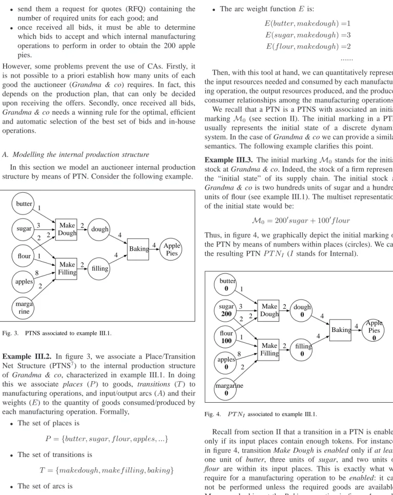
In this section we model an auctioneer internal production structure by means of PTN. Consider the following example.
butter sugar flour apples marga rine Make Dough Make Filling 1 3 2 2 1 8 2 dough filling 2 2 Baking 4 4 Apple Pies 4
Fig. 3. PTNS associated to example III.1.
Example III.2. In figure 3, we associate a Place/Transition
Net Structure (PTNS7) to the internal production structure of Grandma & co, characterized in example III.1. In doing this we associate places (P) to goods, transitions (T) to manufacturing operations, and input/output arcs (A) and their weights (E) to the quantity of goods consumed/produced by each manufacturing operation. Formally,
• The set of places is
P ={butter, sugar, f lour, apples, ...}
• The set of transitions is
T ={makedough, makef illing, baking}
• The set of arcs is
A={(butter, makedough),(sugar, makedough), ...}
.
7Refer to definition II.1.
• The arc weight functionE is:
E(butter, makedough) =1
E(sugar, makedough) =3
E(f lour, makedough) =2
...
Then, with this tool at hand, we can quantitatively represent the input resources needed and consumed by each manufactur-ing operation, the output resources produced, and the producer consumer relationships among the manufacturing operations.
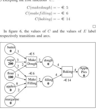
We recall that a PTN is a PTNS with associated an initial marking M0 (see section II). The initial marking in a PTN
usually represents the initial state of a discrete dynamic system. In the case of Grandma & co we can provide a similar semantics. The following example clarifies this point.
Example III.3. The initial markingM0 stands for the initial
stock at Grandma & co. Indeed, the stock of a firm represents the “initial state” of its supply chain. The initial stock at
Grandma & co is two hundreds units of sugar and a hundred
units of flour (see example III.1). The multiset representation of the initial state would be:
M0= 200′sugar+ 100′f lour
Thus, in figure 4, we graphically depict the initial marking of the PTN by means of numbers within places (circles). We call the resulting PTNP T NI (I stands for Internal).
butter 0 sugar 200 flour 100 apples 0 margarine 0 Make Dough Make Filling 1 3 2 2 1 8 2 dough 0 filling 0 2 2 Baking 4 4 Apple Pies 0 4
Fig. 4. P T NIassociated to example III.1.
Recall from section II that a transition in a PTN is enabled only if its input places contain enough tokens. For instance, in figure 4, transition Make Dough is enabled only if at least one unit of butter, three units of sugar, and two units of
flour are within its input places. This is exactly what we
require for a manufacturing operation to be enabled: it can not be performed unless the required goods are available. Moreover, looking at the Baking operation in figure 4, we ob-serve that the producer/consumer relationships between Make
Dough and Baking on one side, and between Make Filling
and Baking on the other side, is quantitatively described by the PTN. Notice that the enabling condition guarantees that
a producer/consumer relationship is not only quantitatively represented, but also it is constrained to be implemented in its dynamics.
If a transition is enabled in a marking it can fire (see definition II.4). If a transition fires it consumes some input goods and produces some output goods. Once more, this is the semantics we require for a manufacturing operation: a manufacturing operation consumes a set of input resources and produces a set of output resources.
Example III.4. In table III we show what happens when the Make Dough transition fires. In the left image Make Dough is
enabled. The execution of Make Dough provides some inputs to the Baking operation, as shown in the image on the right, thus perfectly describing the producer/consumer relationship among them.
What does it happen when there is a sequence of firings? As explained in section II-A, the PTN will pass through a succession of markings (states). In the case of Grandma &
co a marking stands for the state of a production process,
i.e. it describes the resources available at each state of the transformation process. In fact, it associates to each state the number of units of each good available to the auctioneer in that state. Accordingly, a manufacturing operation can be performed in a given state only if enough tokens are available in its input places in that state. The firing of a transition adds tokens into its output places likewise a manufacturing operation produces new available resources to the auctioneer. If markings describe the level of resources currently avail-able to an auctioneer, they naturally apply to describe the requirements of an auctioneer as well. An auctioneer aims at
reaching a marking that fulfils its requirements (at least two
hundreds tokens in the applepie place). This helps linking an auctioneer’s requirements to its internal production structure.
In section II-A, we illustrated the problem of reachability, i.e. the problem of reaching a given marking Md departing
from an initial marking M0. We explained that it is a well
studied problem in the PTN literature. The reader can imagine that the auctioneer is dealing with a similar problem: reaching a marking that fulfils its needs.
Summarizing, by means of the PTN representation we partially fulfill requirements (1) and (2) in table I. However, we still need to express:
• the relationships between the internal manufacturing op-erations and the received offers (limitation (3) in table I); and
• the information about the cost associated to bids’ se-lection and to manufacturing operations’ carrying out (limitation (4) in table I).
Then, in the next section we incorporate the description of the received offers into P T NI.
B. Incorporating Bids
In this section we cope with limitation (3) in table I. That is, to establish a relationship among an auctioneer’s internal production structure, the goods at auction, and the received
offers. This entails relating the PTN description of section III
(P T NI) with the bidders’ offers and the goods at auction.
Firstly, notice that the relation between the auctioned goods and the manufacturing operations is already accounted by
P T NI. It quantitatively specifies the goods required and
produced by each manufacturing operation. Hence, it only re-mains linking the received combinatorial offers to theP T NI.
In fact, the utility of P T NI is very limited if an auctioneer
cannot link it to the received bids. For instance, the PTN (pro-duction process) described in figure 4 cannot work: there are not enough tokens (goods) to fire (run) any of the transitions (manufacturing operations). The problem is that the auctioneer (Grandma & co) needs to buy goods to feed its production process. Buying goods is equivalent to injecting tokens into the corresponding places. For instance, if Grandma & co decides to accept a bid offering 100 units of butter, this will inject 100 units into the butter place and will correspondingly increment the marking of the PTN. The counterpart of this operation would be putting a100into the butter place of figure 4.
As a consequence, incorporating bids into the PTN is quite natural. Indeed, they can be easily modelled by means of tran-sitions as well. If a bid is selected, it must increase the amount of some available resources. Correspondingly, a transition adds tokens into its output places when fired. However, two features distinguish bids from manufacturing operations. Firstly, bids do not consume any resource. Secondly, bids can be run only once (it is not possible to accept a bid twice in our semantics). Therefore, each bid will be represented by a special type of transition, whose single input place will not be a good, but a sort of controller. Such a controller, named bid place, will enforce that a transition representing a bid is selected at most once. We will call this type of transitions bid transitions. In contrast, we will call the transitions corresponding to manufacturing operations operation transitions, and the places representing goods good places. We make clear the process of bid incorporation by means of an example.
Example III.5. Say that Grandma & co receives the
combi-natorial offers in equations (10) to (14) below from bidders. We represent an offer sent by a provider as a multisetB ∈NG,
whereGis the set of goods (in our case represented by places in figure 4), along with a cost. The multiplicity associated to each element of the multiset stands for the number of offered units for the element.
B1→100′butter+ 200′margarine ate200 (10)
B2→200′f lours+ 300′sugar ate100 (11)
B3→800′apples ate200 (12)
B4→200′dough+ 200′f illing ate1300 (13)
B5→200′apple pies ate2400 (14)
For instance,B4→200′dough+200′f illingate1300 stands
for a combinatorial bid offering two hundred units of dough
and two hundred units of filling ate1300.
In figure 5 we intuitively show how to incorporate bids in equations (10) to (14) into theP T NI on figure 4. P T NI is
• • • • • • • • • • Make Dough Make Filling 1 3 2 2 1 8 2 2 2 Baking 4 4 4 • • • • Make Dough Make Filling 1 3 2 2 1 8 2 • • 2 2 Baking 4 4 4 TABLE III
EXECUTION OF A MANUFACTURING OPERATION ONP T NI.
butter 0 sugar 200 flour 100 apples 0 margarine 0 Make Dough Make Filling 1 3 2 2 1 8 2 dough 0 filling 0 2 2 Baking 4 4 Apple Pie 0 4 • B1 100 200 1 • B2 200 300 1 • B3 800 1 • B4 200 200 1 • B5 200 1
Fig. 5. P T NE. Incorporating bids into theP T NIof figure 4.
We will refer to the PTN in figure as the P T NE (E from
Extended). Notice that:
(1) The input places of bid transitions (transitions associated to bids and represented by B1,B2,B3,B4,B5 in figure
5) only contain one token and their input arcs weigh one. Therefore, a bid transition can fire at most once. (2) A bid transition does not have any other input place
except from a bid place. Thus, it does not consume any resources.
(3) The output places of bid transitions are the goods offered in the corresponding bids, whereas the output arcs’ weights are the number of offered units.Therefore, they increase the number of tokens present on the net if fired. In table IV we graphically depict the evolution of the PTN in figure 4 when applying the firing sequence J =
hB1, makedoughi. The upper picture shows the initial
mark-ing M0 = 100′butter + 200′margarine (the stock at
Grandma & co). The central picture shows the marking
obtained after firing transition B1 (i.e. after accepting bid B1). Finally, the lower picture shows the marking obtained
after firing makedough (after performing the Make Dough operation). Notice that in both cases transitions B1and Make
Dough are enabled. Notice also that transitionB1 cannot fire
anymore, whereas Make Dough can.
Summarizing, with the PTN in figure 5 Grandma & co can express:
(1) its internal manufacturing operations along with the pro-ducer/consumer relationships among them (requirement (1) in table I);
(2) the relations among the auctioned goods, the received offers, and the manufacturing operations (requirement (2)); and
(3) its final requirements (requirement (3)).
Furthermore, it can obtain all the possible production states reachable by means of any legal combination of bids and internal operations. That is, it characterizes the combinatorial problem by providing a formalism to enumerate all the pos-sible solutions. This can be achieved thanks to the dynamics of PTN (the firings). This is a crucial point: the P T NE in
figure 5 compactly represents all the possible decisions that
Grandma & co can take.
butter 0 sugar 200 flour 100 apples 0 margarine 0 Make Dough Make Filling 1 3 2 2 1 8 2 dough 0 filling 0 2 2 Baking 4 4 Apple Pie 0 4 • B1 100 200 1 • B2 200 300 1 • B3 800 1 • B4 200 200 1 • B5 200 1 (a) Initially. butter 100 sugar 200 flour 100 apples 0 margarine 200 Make Dough Make Filling 1 3 2 2 1 8 2 dough 0 filling 0 2 2 Baking 4 4 Apple Pie 0 4 B1 100 200 1 • B2 200 300 1 • B3 800 1 • B4 200 200 1 • B5 200 1
(b) After selecting bidB1.
butter 99 sugar 197 flour 98 apples 0 margarine 200 Make Dough Make Filling 1 3 2 2 1 8 2 dough 2 filling 0 2 2 Baking 4 4 Apple Pie 0 4 B1 100 200 1 • B2 200 300 1 • B3 800 1 • B4 200 200 1 • B5 200 1
(c) After performing Make Dough.
TABLE IV
APPLYING THE FIRING SEQUENCEJ=hB1, makedoughi.
reaching a state that fulfils its final requirements, it wants to minimize its costs as well. How can we quantify that performing manufacturing operations costs money? How can we quantify that buying goods costs money? It is under this point of view that PTNs lack of the necessary expressiveness and need to be extended. In the next section, we explain how to deal with such extension.
IV. WEIGHTEDPLACETRANSITIONNETS
There is a feature of some discrete systems (in particular the one we consider) that, to the best of our knowledge, has never been considered so far in the PTN literature, and that we deem fundamental. A change in the state of a system may have an associated cost. For instance, in our case, a manufacturing operation has a cost associated to each time it is carried out. Thus, in order to model manufacturing operations, we need
to extend Place Transition Nets to incorporate the notion of
transition cost. Such extension will allow not only to represent
the fact that a cost is associated to each transition firing, but also to easily compute the cost associated to a firing sequence. One may think to associate a cost to a transition with alternative techniques. For instance, one may insert places that account for the quantity of money needed to perform an operation. Although operationally possible, this extension would constrain the applicability of our method:
• it would not allow expressing fractional quantities • it would reduce the number of solutions by constraining
the order of operation executions. In fact, it would enforce that money is actually present when the transformation takes place, whereas often the operation that injects money is the one at the end of the process.
including more places
Therefore, we present an extension, that we deem being the most natural. However, we do not exclude that one could find alternative solutions to the same problem.
The extension of PTN to incorporate the costs of operations and bids is quite natural and consistent with all the properties of PTN. If we aim at representing the fact that performing a manufacturing operation costs money, we simply have to associate a cost to the firing of an operation transition. Similarly, if we aim at representing that buying goods costs money, we have to associate a cost to the firing of each
bid transition. In general, since both bids and manufacturing
operations can be represented by means of PTNs, we have to associate a cost to each transition in a PTN.
A. WPTNSs and WPTNs
We extend the notion of Place Transition Net (see section II) by associating a cost to each transition. This leads us to the definition of Weighted Place Transition Net Structure (WPTNS) and Weighted Place Transition Net (WPTN).
Definition IV.1 (WPTNS). A WPTNS is a a tuple
(P, T, A, E, C)where:
• P, T, A, E are defined exactly like in a PTNS.
• C : T → R is a cost function that associates a cost to each transition. butter sugar flour apples marga rine Make Dough -e5 Make Filling -e6 1 3 2 2 1 8 2 dough filling 2 2 Baking -e14 4 4 Apple Pies 4
Fig. 6. WPTNS associated to example III.1.
Example IV.1. Let us associate a WPTNS to the internal
production structure of Grandma & co specified in example III.1. At this aim we associate places (P), transitions (T), input/output arcs (A) and their weights (E) exactly like in example 3. The cost function (C) associates a cost to each manufacturing operation. A WPTNS employs the same graphical representation as a PTN (see section II), the only difference being that a cost labels each transition. We depict in figure 6 the resulting WPTNS, formally defined as in example
3 excepting the cost functions8C:
C(makedough) =−e 5
C(makef illing) =−e 6
C(baking) =−e 14
In figure 6, the values of C and the values of E label respectively transitions and arcs.
butter 0 sugar 200 flour 100 apples 0 margarine 0 Make Dough -e5 Make Filling -e6 1 3 2 2 1 8 2 dough 0 filling 0 2 2 Baking -e14 4 4 Apple Pies 0 4
Fig. 7. WPTN associated to example III.1.
Analogously to a PTNS, we define a WPTN by associating to a WPTNS an initial markingM0.
Definition IV.2 (WPTN). A WPTN is a pair(N,M0), where N is s WPTNS, andM0is a multiset of places that stands for
its initial marking.
The initial marking in a PTN represents the initial state of a discrete dynamic systems. The very same semantics is inherited by WPTNs.
Example IV.2. The initial marking M0 for the WPTNS in
figure 6 Grandma & co is:
M0= 200′sugar+ 100′f lour
In figure 7, we graphically depict the initial marking of the WPTNS in figure 6.
B. Dynamics of WPTNs
WPTNSs and WPTNs preserve all the properties of PTNSs and PTNs respectively, but allow the quantitative representa-tion of the cost of a transirepresenta-tion. Therefore, we can naturally extend to them all the concepts employed for PTNs. Those include the concepts of enabling of a transition, firing of a transition, marking, firing sequence, and so on (refer to section II).
In a PTN, if a transition is enabled in a marking it can fire. If a transition fires it consumes some input goods and produces some output goods. In a WPTN, something more happens. If
8The sign convention employed is negative values each time an auctioneer
a transition fires it carries out a cost, the cost associated to the fired transition.
Example IV.3. In table V we show what happens when the Make Dough transition fires. The transition generates a cost of
e5. In the upper right corner we show the quantity of money spent by the auctioneer in the corresponding state.
What does it happen when there is a sequence of firings? Firstly, the WPTN will evolve through a succession of mark-ings (states); and secondly, a cost will be associated to such a sequence of transitions (firing sequence in section II-A). Considering this, we can define the notion of cost of a firing
sequence (CF S) as:
Definition IV.3 (Cost of a firing sequence). The cost CF S
associated to a firing sequenceJ =ht1, t2, ..., tdi is the sum
of all the costs of the transitions contained in the sequence:
CF S(J) =
d
X
i=1
C(ti) (15)
If a transition fires more than once, say k times, then its cost will be added ktimes.
Example IV.4. In figure 8, analogously to figure 5, we
incorporate into a WPTN the bids expressed in equations (10) to (14). Notice that the costs labelling bid transitions is the cost associated to the bids. Furthermore, in table VI, we repeat the firing sequence of table IV (J = {B1, makedough})
when a cost is associated to each transition. In this case, the cost associated to the firing sequence is CF S(J) =
C(B1) +C(makedough) =-e200− e5 =- e205. In the
upper right corner of each frame of table VI we highlight the cost associated to the corresponding firing.
V. REPRESENTING AUCTION OUTCOMES WITHWPTNS In the previous section we introduced WPTNs and showed their powerful modelling features. The examples tried to give the intuitions behind the application of WPTN to our problem. In fact, we saw that the auctioneer faces a
make-or-buy decision problem, and decides to solve it by means of
combinatorial auctions. In this section, we aim at representing each of the outcomes of such auction given a description of the internal manufacturing operations, of the received bids, and of the auctioneer’s final requirements . However, since an auctioneer is mostly interested in assessing the cost associated to each of such outcomes, we also associate an auctioneer’s cost to each of the outcomes.
Then, firstly we introduce the Transformability Network
Structure (TNS), a WPTN for modelling and
communicat-ing the internal manufacturcommunicat-ing operations of an auctioneer. Secondly, we extend the TNS in order to incorporate the information regarding the received bids. This will result in the introduction of the Auction Net. This structure compactly expresses all the possible decisions an auctioneer may take, and quantifies the cost associated to each of such decisions. With those formal tools at hand, we can then define what a MUCRAtR is by providing an operational definition of valid auction outcome.
A. The Transformability Network Structure
In what follows we formally define the Transformability
Network Structure. This corresponds to the net presented in
figure 6. TNSs are useful for expressing the internal man-ufacturing operations of an auctioneer. This tool will have to quantitatively represent the input resources needed and consumed by each manufacturing operation, the output re-sources produced, the producer consumer relationships among the manufacturing operations, and the cost associated to each manufacturing operation. Summarizing, a TNS describes the different ways in which goods can be transformed and at which cost. More formally,
Definition V.1 (TNS). A transformability network structure
is a Weighted Place/Transition Net N = (P, T, A, E,M0, C)
such that we associate:
(1) the places inP to a set of goodsGto negotiate upon9. (2) the transitions in T to a set of internal manufacturing
operations;
(3) the directed arcs inAalong with their weightsEto the specification of the number of units of each good that are either consumed or produced by a manufacturing operation.
(4) the initial marking M0 to the quantity of each good
initially available to the auctioneer (the stock). We indicate this particular initial marking with the multiset
Uin∈NP. Then,M0=Uin.
(5) a costC:T →R+ to each manufacturing operation. In the next section we show how to incorporate the received bids into the TNS. The resulting WPTN is called Auction Net.
Example V.1. The WPTN introduced in example IV.2 is the
TNS associated to the problem of Grandma & co, previously described in example III.1.
Notice that if an auctioneer communicates to bidders its TNS along with some constraints on the final marking (for instance, at least 200 tokens in the apple pie place), the bidders have all the information for composing meaningful offers. This completely fulfills the CAs expressiveness limitation in communicating to bidders an auctioneer’s requirements (issue (2) in table I).
B. The Auction Net
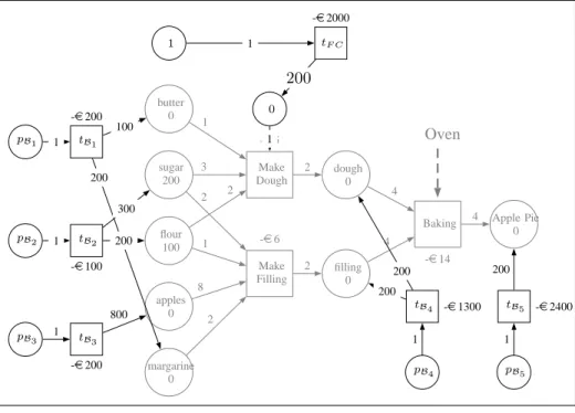
In this section, we will thoroughly explain how to transform a TNS (figure 6) into an Auction net (figure 8). In the remain-ing of the chapter it is assumed that B is the set of received bids. Each bid is represented by a multisetB ∈ NP and has associated a cost encoded by the functionCB:B→R+∪{0}. Definition V.2 (Auction Net). Given a set of bidsB, and a
TNS N = (P, T, A, E,Uin, C), an Auction Net is a WPTN
9Notice that a place represents a good. Thus, in what follows we will
talk indifferently of good places and goods. That is, P and G are employed indifferently.
COST=e0 • • • • • • • • • • Make Dough -e5 Make Filling -e6 1 3 2 2 1 8 2 2 2 Baking -e14 4 4 4 COST=-e5 • • • • Make Dough -e5 Make Filling -e6 1 3 2 2 1 8 2 • • 2 2 Baking -e14 4 4 4 TABLE V
COST OF EXECUTING A MANUFACTURING OPERATION ON AWPTN.
butter 0 sugar 200 flour 100 apples 0 margarine 0 Make Dough -e5 Make Filling -e6 1 3 2 2 1 8 2 dough 0 filling 0 2 2 Baking -e14 4 4 Apple Pie 0 4 • B1 -e200 100 200 1 • B2 -e100 200 300 1 • B3 -e200 800 1 • B4 -e1300 200 200 1 • B5 -e2400 200 1
Fig. 8. Incorporating bids into the WPTN of figure 7.
butter 0 sugar 200 flour 100 apples 0 margarine 0 Make Dough -e5 Make Filling -e6 1 3 2 2 1 8 2 dough 0 filling 0 2 2 Baking -e14 4 4 Apple Pie 0 4 Oven pB1 tB1 -e200 100 200 1 pB 2 tB2 -e100 200 300 1 pB 3 tB 3 -e200 800 1 pB 4 tB4 -e1300 200 200 1 pB 5 tB5 -e2400 200 1
Fig. 9. Auction Net of the MUCRAtR in example III.1.
S∗= (P∗, T∗, A∗, E∗,M∗ 0, C∗)where: P∗ =P∪P B T∗ =T ∪TB A∗ =A∪A B
(1) PB is the set of bid places. That is, for each bidB ∈B
add a place pB.
COST=e0 butter 0 sugar 200 flour 100 apples 0 margarine 0 Make Dough -e5 Make Filling -e6 1 3 2 2 1 8 2 dough 0 filling 0 2 2 Baking -e14 4 4 Apple Pie 0 4 • B1 -e200 100 200 1 • B2 -e100 200 300 1 • B3 -e200 800 1 • B4-e1300 200 200 1 • B5-e2400 200 1 (a) Initially. COST=-e200 butter 100 sugar 200 flour 100 apples 0 margarine 200 Make Dough -e5 Make Filling -e6 1 3 2 2 1 8 2 dough 0 filling 0 2 2 Baking -e14 4 4 Apple Pie 0 4 B1 -e200 100 200 1 • B2 -e100 200 300 1 • B3 -e200 800 1 • B4-e1300 200 200 1 • B5-e2400 200 1
(b) After selecting bidB1.
COST=-e205 butter 99 sugar 197 flour 98 apples 0 margarine 200 Make Dough -e5 Make Filling -e6 1 3 2 2 1 8 2 dough 2 filling 0 2 2 Baking -e14 4 4 Apple Pie 0 4 B1 -e200 100 200 1 • B2 -e100 200 300 1 • B3 -e200 800 1 • B4-e1300 200 200 1 • B5-e2400 200 1
(c) After performing Make Dough.
TABLE VI
APPLYING THE FIRING SEQUENCEJ=hB1, makedoughi.
B ∈B add a transitiontB.
(3) AB is the set of bid arcs. It is built as follows:
AB =AiB∪AoB
where
AiB ={(pB, tB)∈PB×TB | ∀B ∈B} (16)
Ao
B ={(tB, p)∈TB×P |p∈ B} (17)
are the input bid arcs and output bid arcs respectively. (4) The arc expression E∗ function is built as follows:
E∗(x, y) =E(x, y) (x, y)∈A (18)
E∗(tB, p) =B(p) (tB, p)∈AoB (19)
E∗(pB, tB) = 1 (pB, tB)∈AiB (20)
(5) The cost functionC∗:T∪T
B →Ris built as follows:
C∗(t) =C(t) t∈T
C∗(tB) =CB(B) tB∈TB
(6) The initial marking is defined as
M∗ 0(p) = ( Uin(p) p∈P 1 p∈PB (21)
Example V.2. We extend the TNS of example IV.1 with the
bids listed in equations (10) to (14). This gives raise to the
Auction Net in figure 9. (P, T, A, E,M0, C) have been
de-fined in example IV.1. Then,S∗= (P∗, T∗, A∗, E∗,M∗
0, C∗)
is defined as follows:
(2) T∗=T∪ {t B1, tB2, tB3, tB4, tB5} (3) A∗=A∪Ai B∪AoB where Ai B={(pB1, tB1),(pB2, tB2),(pB3, tB3), ...} AoB={(tB1, butter),(tB1, margarine), . . .} (4) E∗(x, y) = E(x, y) if (x, y)∈ A. When (x, y) ∈ A B we have: E∗(tB1, butter) = 100 E ∗(t B1, margarine) = 200 E∗(tB2, sugar) = 300 E ∗(t B2, f lour) = 200 . . . . E∗(pB1, tB1) = 1 E ∗(p B2, tB2) = 1 . . . . (5) C∗(t) =C(t)when t∈T. Whent∈T B we have: C∗(tB1) =-e200 C ∗(t B2) =-e100 C∗(tB3) =-e200 C ∗(t B4) =-e1300 C∗(tB5) =-e2400
Recall that by means of the PTN defined in example III.5, an auctioneer was able to compactly represent all the possible outcomes associated to any of its decisions. However, he had the problem to assess the cost associated to each of such outcomes. Notice that by means of the auction net, the auctioneer can now express both the outcomes of its decisions and the cost associated to each of them.
In order to define the winner determination problem for MUCRAtR one further step is required. We have to define an optimization problem whose solution retrieves the optimal firing sequence to apply to the auction net in order to obtain a desired final marking (in the case of Grandma & co more than 200 tokens in the apple pie place). This is the purpose of the following section.
C. Constrained Maximum Weight Occurrence Sequence Prob-lem
Since there is a cost associated to each transition, one may be interested in finding a maximum (minimum10) cost firing sequence leading from an initial marking to some final marking. More importantly, one may be interested in finding a maximum cost firing sequence leading from an initial marking M0 to a final marking Md that fulfils a set of inequality constraints. For instance, we may want to impose
that in a final marking Md each place contains exactly one
token (Md(p) = 1,∀p ∈ P), or at least 200 tokens in a
given place (for instance, the Apple Pie place in example III.1 Md(applepie) ≥ 200). With this aim we define the Constrained Maximum Weight Occurrence Sequence Problem
(CMWOSP).
Definition V.3 (CMWOSP). Given a WPTN N =
(P, T, A, E,M0, C), a set of inequality/equality constraints
10In any optimization problem maximizing and minimizing are two dual
representations of the very same problem. We will talk about maximization in what follows, but all the results can be easily applied to a minimization.
that a final markingMd must fulfil, expressed as:
∀p∈P Md(p)∆php (22)
where ∆p ∈ {<,≤,=,≥, >} and hp ∈ N∪ {0}, find an
occurrence sequence Jopt = hu1, u2, ..., udi that brings the
initial marking M0 to a final marking Md such that: (1) Md fulfils all the constraints in equation (22); and (2) Jopt
maximizes the total cost CF S.
We can express the inequations (22) in matrix form:
Md∆h (23)
whereMd is a vector whosei−thcomponent represents the
number of tokens in place i, ∆ is a vector whose i−th
element contains {<, >,≤,≥,=}, and h is a vector whose
i−th element contains hp. We will call the constraints in
equation (22) or (23) the final marking constraints.
Proposition V.1. CMWOSP is at least EXPSPACE-hard. Proof: The reachability problem for PTN can be reduced
to a CMWOSP. It has been proved that the reachability problem is EXPSPACE-hard [43].
VI. THEWINNERDETERMINATIONPROBLEM In this section, we formally define the winner determination
problem for MUCRAtR.
Informally, given a TNS expressing the internal manufac-turing operations of an auctioneer over a set of goods G, an auctioneer’s final requirements Uout ∈ NG, and a set of
received bids B, the winner determination problem amounts to finding the set of bids and internal operations that minimize the auctioneer’s cost and produce at least the required goods. The formal definition of the WDP relies on the Auction Net.
Definition VI.1 (Winner Determination Problem). Given
an auction expressed as hN,Uout, Bi, where N =
(P, T, A, E,M0)is a TNS,Uout∈NGexpresses the
auction-eer final requirements, andB is the set of received bids. Let
S∗= (P∗, T∗, A∗, E∗,M∗
0, C∗)be the corresponding Auction Net. The Winner Determination Problem amounts to selecting
the set of bidsB∗ and the sequence of internal operationsJ∗
that both minimize the auctioneer’s cost and satisfy the the following final marking constraints on the Auction Net:
Md(p)≥ Uout(p) ∀p∈P (24)
Md(p)≥0 ∀p∈PB (25)
Proposition VI.1. The WDP for a MUCRAtR hN,Uout, Bi can be reduced to a CMWOSP on the corresponding auction net. Such a CMWOSP is characterized by the following final
marking constraints:
Md(p)≥ Uout(p) ∀p∈P (26)
Md(p)≥0 ∀p∈PB (27)
Proof: The proof is by construction:
(1) Solve the CMWOSP on the Auction Net NB. We name