Fear Trading

(1)

MPRA

Munich Personal RePEc Archive

Fear Trading

Ardia, David

Swiss Federal Institute of Technology Zurich

2003

Online at

http://mpra.ub.uni-muenchen.de/12983/

(2)

Fear Trading

Julien Dinh and David Ardia1

June 2003

Abstract

Our trading strategy is inspired from the paper ’implied volatility indices as leading indicators of stock index returns?’, Giot (2002,[3]). It uses stylized facts observed in stock markets: the so called ’leverage effect’, the clustering and the mean-reverting behaviour of the implied volatility. Based on S&P100 and VIX data, we show that abnormally high levels of volatility can be used as a trading signals for long traders. A bootstrap procedure confirms the signifi-cant returns for the 1986-2003 period.

1

Master of Advanced Studies in Finance, 2003, University of Zürich and Swiss Federal Institute of Technology; mailing addresses: [email protected] and [email protected]

(3)

1 Introduction

Many studies have shown that the volatility is time dependent and follows a mean reverting process. In addition we observe that the volatility fluctuates cyclically around a certain mean level which varies over time. This stylized fact is referred as the ’volatility clustering’.

We recall that the ’leverage effect’ has its origin in the observation that volatility is negatively correlated with stock returns. The first explanation to this empirical fact was given by Black and Christie (see [1], [2]) in the sense that negative returns increase financial leverage which extend the risk of the company and therefore its volatility. Another possible explanation to the negative correlation is, that the fear induced by an increase of volatility produces a fall of demand and hence a price decrease.

Our trading strategy is based upon the above mentioned properties. We detect periods of abnormally high (low) volatility and take a long (short) position accordingly. The position is kept open until the volatility returns to a ’normal’ level. Gains should arise from negative correlation between returns and volatility. The remaining part of the paper is organized as follows. Section 2 presents the data used for our analysis. Section 3 explains the methodology of our trading strategy and presents the results for our long and short strategy. In section 4 we compare results to other quantile based strategies and apply a bootstrap performance measure. Section 5 concludes.

2 Data

2.1 Data used

We test our trading strategy on daily closing values of the S&P100 index. Since volatility is a basis for our trading strategy, we need to define it. The first candidate is the historical volatility. Many studies have shown the poor quality of prevision of this estimator and its poor ability to react quickly on new information (see [5],[8]). In addition, as the construction of this proxy depends on the observation window, estimations can vary significantly, and hence would not represent the general view of investors. Therefore we decide to focus on an other indicator. The implied volatility is the next natural candidate. This indicator does not overperform the historical approach (see [7],[6]) but has many advantages. First as it is implied from actively traded options, it represents the best assessment by investors on the expected future volatility. Second, a common volatility index is computed continuously by the CBOEc

and is freely provided to investors. For these reasons we use the S&P100 implied volatility index, the VIX. Since the VIX index started on the 2-JAN-1986, we use the complete history until the 28-MAR-2003 for both series. The data were downloaded from www.yahoo.finance.com.

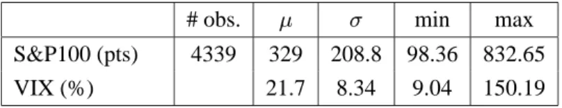
# obs. min max

S&P100 (pts) 4339 329 208.8 98.36 832.65

VIX (%) 21.7 8.34 9.04 150.19

Table 1: Some statistics on data

The table 1 presents the number of observations, the mean, the volatility, the minimum and the maximum value of S&P100 and VIX indices. The observation window ranges from 2-JAN-1986 to 28-MAR-2003.

(5)

2.2 Data analysis

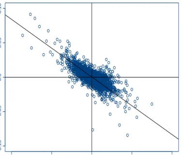
To show an example of the negative correlation between stock and volatility, we compute continuous returns2of both indices for the whole period. The figure 1 shows a clear negative cross-sectional correla-tion between the two returns. A linear regression exhibits a negative slope at a level of -0.83 (t-stat=-70) and a R2

of 54%.

abnormal vol changes (%)

return changes (%) -0.10 -0.05 0.0 0.05 0.10 -0.10 -0.05 0.0 0.05 0.10

Figure 1: negative correlation

Figure 1 presents a scatter plot of daily stock returns and daily abnormal volatility returns over the whole observation window. The slope of the linear regression is -0.83. The R2

is 54%

To use the empirical fact of negative correlation as a trading signal, we need to predict future volatility movements. The underlying idea is to use the mean-reversion which implies that in extremely high (low) volatility periods, there is a high probability of a return to ’normal’ levels. To quantify normal levels of volatility, we use a moving average over the last trading year (250 days).3We then compute the abnormal volatility defined as ab;t := t t

From there we quantify the level of abnormal volatility (AV) by its position in the historical distribution.4. Abnormal volatility and quantiles are the information used for our trading rule.

2 rt:=ln(St=St 1) 3 t:= 1 250 P 249 i=0 t i 4_{quantiles at 99% ; 95% ; 90% ... ; 5% ; 1%}

(6)

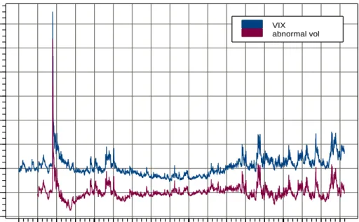
1986 1987 1988 1989 1990 1991 1992 1993 1994 1995 1996 1997 1998 1999 2000 2001 2002 2003 0 20 40 60 80 100 120 140 date volatility (%) VIX abnormal vol

Figure 2: VIX index and abnormal volatility

This figure 2 presents the evolution of the implied volatility index VIX (above) and the abnormal volatility computed using a moving average window of 250 days. The observation window ranges from 2-JAN-1986 to 28-MAR-2003

3 Trading strategy and results

To test the power of our leading indicator for future index returns, we define a long (short) strategy based on abnormally high (low) volatility periods.

3.1 Description of the strategy

Our strategy going long in the index is based on the idea that investors are mean variance optimizers. When the abnormal implied volatility increases, the expected Sharpe ratio of the stock universe decreases which could be interpreted as a signal that investors will go out of stock market. At this point, the volatil-ity increases even more (leverage effect) and reaches the highest quantiles of it’s implied distribution. Then, the mean reversion property of the implied volatility enters and drags the volatility back to ’nor-mal’ levels, leading to an increased stock value. For this reason, the abnormal implied volatility is our sole source of information. We decompose our strategy in 4 phases depending on the AV level:

1. AV is low ! wait

2. AV reaches the 99th quantile ! warning

3. AV decreases under the 99th quantile ! buy one index

4. AV decreases under the 85th quantile ! sell one index

(7)

Since we want to take a long position in the index, we need to detect moments having high probability of decrease in AV. This happens when the AV reaches levels haven’t been attained for the past year. We measure these moments using the 99th quantile of the historical AV distribution (step 2 in table 2). To have an additional signal of a future decrease, we wait until the AV crosses the 99th quantile from above and open the position (step 3 in table 2). We want to keep the position open until investors fear has disappeared and while the AV decreases. We define the exit quantile as the 85th (step 4 in table 2). Figure 3 decrypts this strategy for on a given position. On October 5th, AV reaches the 99th quantile and the investor becomes aware. On October 8th, AV crosses the 99th quantile on a downward trend; the investor goes long in the index. He closes his position on October 25th since the 85th quantile is reached.

Sep 28 Oct 5 Oct 12 Oct 19 Oct 26 Nov 2

1992 -1 0 1 2 3 4 5

Sep 28 Oct 5 Oct 12 Oct 19 Oct 26 Nov 2

1992 29 30 31 32 33 34 35

Figure 3: Long strategy

On the left hand-side, the figure 3 presents the evolution of the 99-quantile (above), the 85-quantile (below) and the abnormal volatility over a 2 month observation window. The long position is open October 8th (upward triangle) and is closed October 25th (downward triangle). On the right hand-side, the figure presents the evolution of wealth in the portfolio for the same period. Moreover, we clearly remark the opposite behaviour of the two time series highlighting the negative correlation property.

The short strategy is symmetric to the long one and can be summarized by the table below:

1. AV is high ! we wait

2. AV reaches the 15th quantile ! warning

3. AV increases over the 15th quantile ! sell one index

4. AV increases over the 30th quantile ! buy back one index

Table 3: Steps of the short strategy

As our trading strategy is based on the volatility mean reversion, we need to find an entry quantile which indicates a high probability of future volatility increase. Since the market can drift for a long period with a very low volatility, we do not think that the lowest quantiles are very good indicators. Therefore, we do not chose the 1st quantile as an entry signal for the short strategy. We arbitrarily chose the slightly

(8)

higher 15th quantile as the lowest quantile signaling a return to normal levels of volatility. As in the long position, we take 15% difference between entry and exit quantiles, hence we exit at the 30th quantile. The assumptions for the long and short strategies are:

borrowing rate (BR): 9% lending rate (LR): 5% beginning capital : $0 long strategy

- gains (losses) are invested at the LR (BR).

- additional (rest) capital needed to buy the share is borrowed at BR (lent at LR).

short strategy

- strategy are invested at the LR (BR).

- money received from shorting the stock is kept by the broker until we buy back the share.

3.2 Results

This section presents results for our strategies: the long 99-85%, the short15-30% and their combination. Both strategies start on the 22-DEC-1987 and end on the 28-MAR-2003. We start the strategies 500 days after the first observation because we need 250 days to construct the moving average and 250 days for the quantiles.

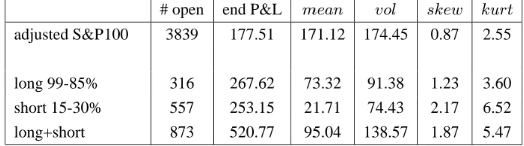
# open end P&L mean vol skew kurt

adjusted S&P100 3839 177.51 171.12 174.45 0.87 2.55

long 99-85% 316 267.62 73.32 91.38 1.23 3.60

short 15-30% 557 253.15 21.71 74.43 2.17 6.52

long+short 873 520.77 95.04 138.57 1.87 5.47

Table 4: Summary of P&Ls

Table 4 presents the results of the long 99-85% and short 15-30% strategies as well as the combination. The first row gives results for the adjusted S&P100 (S&P100 minus the compounded interest rate, LR=5%). Columns give number of open days, the final P&L, the mean, the volatility, the skewness and the kurtosis in $ of the strategies.

(9)

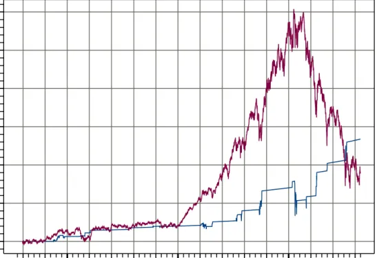
Figure 4 shows the daily P&L evolution for the 99-85% strategy. Results are compared with the adjusted S&P100 index (defined as the buy-and-hold strategy (BH)), that is the value of the index minus the compounded interest rate at the lending rate (LR=5%) to penalize5our trading strategy. We take position only 8% of the time (316 over 3839 days) but the P&L profile clearly shows that the strategy captures positive index price jumps. Moreover, the strategy performs as well during bullish (1988-2000) and bearish (2000-2003) periods. The final P&L reaches $267, $90 higher than in the BH case.

evoltion of the P&L

1988 1989 1990 1991 1992 1993 1994 1995 1996 1997 1998 1999 2000 2001 2002 2003 0 100 200 300 400 500 600

Figure 4: strategy 99-85% against the adjusted S&P100

Figure 4 presents the daily P&L evolution for the long strategy 99-85% (below) and the adjusted S&P100 (above). The observation window ranges from 2-JAN-1987 to 28-MAR-2003. The adjusted S&P100 is defined as the value of the S&P100 index minus the compounded interest rate (LR=5%).

5

(10)

Figure 5 presents the 15-30% daily P&L evolution. The number of open positions represents 14.5% of the whole period and hence is twice more exposed to market risk. We obtain a negative P&L during the bullish period with low volatility (13% for 1987-1997 and 22% for 1997-2003). The minimum P&L reached on the 27-JUNE-1997 is $-45.14. However, for the second part of the observation window, the strategy P&L increases quickly and reaches $253, $76 higher than a simple BH strategy. The profile of the P&L suggests that it could be used to hedge a long position.

evoltion of the P&L

1988 1989 1990 1991 1992 1993 1994 1995 1996 1997 1998 1999 2000 2001 2002 2003 0 100 200 300 400 500 600

Figure 5: strategy 15-30% against the adjusted S&P100

Figure 5 presents the P&L evolution for the short strategy 15-30% (below) and the adjusted S&P100 (above). The observation window ranges from 2-JAN-1987 to 28-MAR-2003. The adjusted S&P100 is defined as the value of the S&P100 index minus the compounded interest rate (LR=5%).

(11)

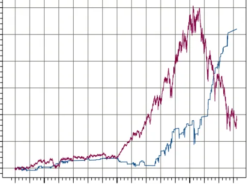
When we combine both strategies, we obtain results given in figure 6. The P&L underperforms the BH strategy until mid 2001, but clearly overperforms it in the second part to reach $520, $343 more than the BH. The combination of a strategy which capture the growth opportunity of the index and a second strategy which works as a portfolio insurance gives very significant results.

evoltion of the P&L

1988 1989 1990 1991 1992 1993 1994 1995 1996 1997 1998 1999 2000 2001 2002 2003 0 100 200 300 400 500 600

Figure 6: strategy 99-85% + 15-30% against the adjusted S&P100

Figure 6 presents the evolution of the P&L of long 99-85% + short strategy 15-30% (below) and the adjusted S&P100 (above). The observation window ranges from 2-JAN-1987 to 28-MAR-2003. The adjusted S&P100 is defined as the value of the S&P100 index minus the compounded interest rate (borrowing=5%).

3.2.1 Robustness

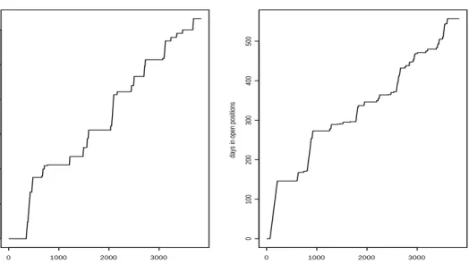
To understand previous results, we analyse the date distribution of entering signals. To do so, we com-pute cumulative sums of open positions for long and short strategies (see figure 7). For both strategies, positions are held throughout the period with a slightly higher proportion at the beginning. Since figures 4 and 5 have shown that the returns are made on the second part of the trading window our performance does not come from a long lasting open position during the bullish (bearish) market. Moreover, we notice that the loss observed at the beginning of the short strategy is mainly due to an open position of 145 days. The very high volatility during the October 1987 crash has biased our estimator of ’normal’ volatility (see in figure 2 the low AV for 1988).

(12)

days

days in open positions

0 1000 2000 3000 0 50 100 150 200 250 300 long 99%-85% days

days in open positions

0 1000 2000 3000 0 100 200 300 400 500 short 10%-30%

Figure 7: Distribution of open positions

Figure 7 presents the cumulative sum of open positions for both strategies analysed in section 3.2. Horizontal segments repre-sents closed positions. Segments with slope of 1 reprerepre-sents open positions. The observation window ranges from 2-JAN-1987 to 28-MAR-2003.

4 Performance measurement

Since our trading strategy is dynamic and takes open positions only 8% and 14% of the whole period, it is clearly not consistent to compare it with a simple buy-and-hold strategy for which the set of information does not change over time. When we compute the Sharpe ratio of strategies we are faced with two additional problems. First, as our strategy needs zero initial investment, movements in the invested share will affect strongly the value of our portfolio, and hence produce extremely high volatility. Second, even if our strategy produces mainly positive returns on a position, the induced volatility, in fact beneficial for the investor, would penalize the Sharpe ratio. To tackle the problem, we have thought to use as a proxy of risk the variance of negative returns and compute the Sharpe ratio accordingly. However, the lack of negative returns does not provide accurate estimation of the volatility. Once again, the performance measure is not relevant. Conscious of these different problems, we decide to focus on a comparative approach with other quantiles strategies and a bootstrap procedure.

4.1 P&L comparison

In that section, we compare results of our two strategies against all other possible quantile strategies. The aim is to determine whether trading extremes generates higher returns than comparable strategies. We perform 54 long strategies with {99, 95, 90, ..., 55%} as entry and {95, 90, ..., 50%} as exit quantile. Similarly, short strategies are applied with {1, 5, 10, ..., 45%} as entry and {5, 10, ..., 50%} as exit quantile.

(13)

4.1.1 Long strategies

Figure 8 (left) provides final P&Ls for all long strategies. The first observation is that all strategies besides the 55-50% have positive P&Ls. It seems that the higher the entrance quantile is, the higher the final P&L. For a zero-investment capital, results range from $-4.28 (55-50%) to $299 (99-50%). Over all strategies, final P&Ls have a mean of $161.7 and a standard deviation of $78.4. In addition, within each entrance quantile, the lower the exit quantile is, the higher the return. For instance with an entrance quantile at 99%, we obtain the following P&Ls: {$141, $252, $267, $252, $261, $265, $204, $274, $279, $299}. strategy number end P&L 0 10 20 30 40 50 0 100 200 300 99 95 90 85 80 75 70 65 6055 long strategy strategy number end P&L 0 10 20 30 40 50 0 100 200 300 1 5 10 15 20 25 30 35 4045 short strategy

Figure 8: strategies final P&L

The figure 8 presents final P&Ls for all strategies. On the left hand-side, results for long strategies are provided with entry quantile {99, 95, 90, ..., 55%} noted on the top of the graph. On the right hand-side, results are given for short strategies. Entry quantiles are given on the top of the graph {1, 5, 10, ..., 45%}.

However, these results have to be analyzed carefully. As each strategy corresponds to a different number of positions, we should take account for market exposure. Therefore, when we divide the final P&L by the number of days in open position, we clearly see that previous results no longer hold (figure 9 left). Here we observe an exponential increase with respect to the entry quantile. Using this criteria, our long strategy (99-85%) ranks 3rd out of 55.

(14)

strategy number

return in $ per day during open position

0 10 20 30 40 50 -0.2 0.0 0.2 0.4 0.6 0.8 1.0 99 95 90 85 80 75 70 65 6055 long strategy strategy number

return in $ per day during open position

0 10 20 30 40 50 -0.2 0.0 0.2 0.4 0.6 0.8 1.0 1 5 10 15 20 25 30 35 4045 short strategy

Figure 9: strategies $P&L per open days

The figure 9 presents P&Ls per day of open position for all strategies. On the left hand-side, results for long strategies are provided with entry quantile {99, 95, 90, ..., 55%} noted on the top of the graph. On the right hand-side, results are given for short strategies. Entry quantiles are given on the top of the graph {1, 5, 10, ..., 45%}.

4.1.2 Short strategies

Figure 8 (right) presents final P&Ls for all short strategies. We still observe positive P&Ls for 49 out of 55 strategies. The general distribution of P&Ls is maximum for strategies entering between 10% and 25% quantiles and looks like an inverted U shaped curve. For a zero-investment capital, results range from $-65.96 (5-15%) to $302.5 (20-45%). In addition, within each entrance quantile it seems that the higher the exit quantile, the higher the return. For instance with an entrance quantile at 10%, we obtain the following P&Ls: {$52, $114, $232, $241, $256, $262, $260, $182}. However for all strategies, waiting too long (exit at the last 50% quantile) leads to substantial decrease in P&L. When we divide P&Ls by the number of open days (figure 9 right), we still keep the inverted U shaped curve. Using this criteria, our short strategy (15-30%) ranks 7 out of 55.

4.2 Bootstrap procedure

The aim here is to determine whether our trading rule (99-85 and 15-30%) provides good market timing. To assess this conclusion, we simulate random shifts of our entry dates and compare the cumulative returns.

For the two strategies we determine the lengthl

iand return r

iof the

ith position. We then construct the

cumulative return defined by

R:= N Y i=1 (1+r i )

(15)

whereN is the total number of positions in the strategy. Then, using a resampling procedure based on

Dirichlet partitioning, we randomly generate N entry dates and compute observed returner ion the

l

inext

days. From the observed returns we calculate the cumulative return e

R for the series. We repeat this

sampling procedure 20’000 times for both long and short strategies.

Figure 10 presents the cumulative returns for both long and short simulations. Results are very different for long and short strategies. Market timing is clearly observed for the long strategy, whereas the short strategy provides an average performance.

Long

Total cumulated return

Frequency 0.5 1.0 1.5 2.0 2.5 0 20 60 100 Short

Total cumulated return

Frequency

0.5 1.0 1.5 2.0 2.5 3.0 3.5

0

50

150

Figure 10: Bootstrap distributions

Figure 10 presents simulated cumulative returns distributions. 20’000 simulations are performed using Dirichlet algorithm. The cumulative return is defined byR:=

Q N i=1

(1+ri), whereriis the return on theith position andNis the total number of positions. The vertical line is the cumulative return for our strategies (99-85% long and 15-30% short).

(16)

simulated e R

R min 25th 50th 75th max

long 99-85% 1.97 0.91 0.24 0.41 0.76 0.86 0.99 2.61

short 15-30% 1.34 1.25 0.41 0.19 1 1.25 1.51 3.42

Table 5: Results of bootstrap

Table 5 presents a summary of cumulative returns for observed and simulated strategies. The first columnRgives cumulative return for observed strategies. e

Rdenotes results for resampling simulation. It givesthe mean,the standard deviation and some quantiles of the simulated distribution. The bootstrap procedure was performed 20’000 times.

5 Conclusion

In this paper, we try to assess the performance of volatility as leading indicator for future stock returns. In order to determine future changes in volatility, we use its mean reverting behaviour. Since volatility will stay bounded, high (low) volatility have a high probability of future decrease (increase). Hence, extremes are signals for our trading rule.

The two performance measurement made in section 4 reveal different results. For the 99th quantile, the analysis seems to assess that it is a good indicator of future stock movements. On the contrary, the 15th quantile ranks 7 out of 55 in short strategies, but has an average performance in the bootstrap measurement. Therefore we can conclude that low quantiles are weak indicators. This difference can be explained by two opposite investors behaviour in periods of high and low volatility. Periods of high volatility are linked to a stress environment and excess fear selling. Hence, the market will jump and the return to ’normal’ market volatility will be made over a short period of time. On the contrary, when low volatility is reached, investors will keep their position creating a slow return to ’normal’ market volatility.

The conclusion of our analysis is that extreme volatility trading is only profitable for high volatility. Returns of our long strategy could be associated to a ’fear premium’ due to the market riskiness in high volatility periods. A further step to our paper would be to include the negative impact of risk capital requirements within the strategy.

(17)

References

[1] F.BLACK; 1976; Studies of Stock Price Volatility Changes; Proceedings of the 1976 Meetings of the Ameri-can Statistical Association; Business and Economic Statistics Section; 177–181;

[2] A.CHRISTIE; 1982; The Stochastic Behavior of Common Stock Variances: Value, Leverage and Interest Rate Effects; Journal of Financial Economics; 3; 407–432;

[3] P.GIOT; 2002; Implied volatility indices as leading indicators of stock index returns? CORE DP 2002/50; [4] P.GIOT; 2002; The information content of implied volatility indexes for forecasting volatility and market

risk;

[5] L.CANINA and S.FIGLEWSKI; 1993; The information content of implied volatility; Review of Financial Studies; 6;

[6] S.Poon and C.Granger; 2003; Forecasting volatility in financial markets: a review; Forthcoming in the Journal of Economic Literature.

[7] B.J.CHRISTENSENand N.R.PRABHALA; 1998; The relation between implied and realized volatility; Journal of Financial Economics 50;

[8] BJ.BLAIR, S.POON and S.J.TAYLOR; 2001; Forecasting S&P100 volatility: the incremental information content of implied volatilities and high-frequency index returns, Journal of Econometrics 105;

Appendix

Long Return of positions Frequency 0 2 4 6 8 10 0 1 2 3 4 5 Long Return of positions Frequency 0 2 4 6 8 10 0 1 2 3 4 5 Short Return of positions Frequency −1 0 1 2 3 4 5 0 1 2 3 4 5 Short Return of positions Frequency −1 0 1 2 3 4 5 0 1 2 3 4 5

Figure 11: Distribution of the cumulative returns

Figure 11 presents distributions for annualized position returns ri( 250 l i )

. The left hand-side shows results for 99-85% long strategy and the right hand-side for the 15-30% short strategy. We notice here a small number of negative returns for both strategies.