Cloud-based Scalable Object Detection and
Classification in Video Streams
Muhammad Usman Yaseen, Ashiq Anjum, Richard Hill, Omer Ranaa College of Engineering and Technology, University of Derby, UK
aSchool of Computer Science and Informatics, Cardi↵University, UK
Abstract
Recent advances in cameras, cell phones and camcorders – particularly the resolution at which they can record an image/ video, are generating large amounts of data. This video data is often so large that manually inspect-ing it for useful content can be time consuminspect-ing and error prone – thereby requiring automated analysis to extract useful information & metadata. Au-tomated analysis often involves approaches to detect, track and recognize objects. But most of these approaches address challenges that are applica-ble to still images. These approaches operate under a supervised learning domain, requiring substantial amounts of labelled data and training time. There is still a wide gap present in terms of processing of video data and in extracting meaningful information from it. We present a cloud-based, au-tomated video analysis system to process a large number of video streams, and enabling the underlying infrastructure to scale based on the number and size of the stream(s) being considered. The system automates the video analysis process and reduces the involvement of human factor. An operator using this system only specifies the object of interest which is to be located from the video streams. The video streams are then automatically fetched from the cloud storage and analyzed in an unsupervised way. Objects are extracted from video streams independently and then object recognition is performed for identification. All the specified objects can be classified from the video streams without requiring any metric learning stage and costly la-belled training data. The proposed system locates and classifies an object of
Email addresses: [email protected](Muhammad Usman Yaseen),
[email protected](Ashiq Anjum),[email protected](Richard Hill),
interest from one month of recorded video streams comprising 175GB size on a 15 node cloud in 6.52 hours. The GPU powered infrastructure took 3 hours to accomplish the same task. Occupancy of GPU resources in cloud is opti-mized and data transfer between CPU and GPU is miniopti-mized to achieve high performance. The system is independent of any metric learning stage and costly labeled training data. The scalability of the system is demonstrated along with a classification accuracy of 95%. The system reduces processing time by up to 90x when compared to analysis of full frames (tested on a large number of video streams).
Keywords:
Unsupervised Object Classification, Cloud Computing, GPUs, High Performance Video Analytics.
1. Introduction
The increasing availability and deployment of video cameras has resulted in the generation of thousands of high resolution videos streams. Such a video can be sub-divided into a number of frames of interest. Various types of information can be extracted from these video frames, such as classification of moving objects corresponding to a specific area of interest. The term video analytics refers to the optimized processing of these video frames by using intelligent approaches such as a machine learning, so that clusters of information can be extracted from them.
Video analytics systems mainly perform object detection and recogni-tion. Object detection refers to the detection of all instances of an object belonging to a known category, such as faces or cars, within a sequence of frames. Often a video may contain a number of objects. These objects can reside at any location within a frame – requiring the detection process to investigate di↵erent parts of the frame to locate the object of interest. Ob-ject recognition, on the other hand, refers to the identification of detected objects. Labels are assigned to the detected objects during this process. A video stream and some known labels are provided to the system. It then assigns the correct labels to the detected objects in a video stream. [1][2][3] describe how video frame analysis can be used to support detection, track-ing and recognition of objects. But these systems are expensive in terms of processing time and cost [4], require human monitoring and intervention [5] and address challenges that are often relevant for still images [6]. These
systems require a large number of resources such as operators and working place. Due to cognitive limitations, an operator cannot focus on recorded video streams for more than 20 minutes; making it unfeasible to perform efficient and robust large scale video analysis. Scaling such analysis to large data volumes also remains a challenge. Additionally, to gain greater insights into the analysed video content, computationally intensive algorithms (e.g. deep learning algorithms [7]) with large storage requirements are needed.
This work utilizes the advantages of machine learning based classification approaches to develop an automated video analysis system which overcomes these challenges. The focus of this work is to build a cloud based robust and scalable solution for the processing of large number of video streams. We employed the detection and classification algorithms in combination in order to combine the benefits of both supervised and unsupervised learn-ing domains. The Haar Cascade Classifier [8] has been demonstrated to be highly accurate for object detection, especially for detecting faces in still images [10]. We have therefore investigated its use for video sequences. Sim-ilarly, Local Binary Pattern Histogram [9] is a widely used classification algo-rithm, primarily because of its computational simplicity and high accuracy. Our system requires minimum human interaction for identifying objects in a large number of video frames. The system is based on a very simple object matching concept. After the extraction of desired objects, we employed the object matching algorithm to perform object recognition. This enabled us to perform classification without any metric learning algorithm and labelled training data.
An operator using the system only specifies the object of interest which is to be located. The video streams are then automatically fetched from the cloud storage and processed frame by frame. The moving object is first detected in a frame to provide a reference for the location of the object which can be tracked in the subsequent frames. It is cropped and saved at a separate image, so that the recognition step will have to process a smaller sized image. The moving object is then passed on to the subsequent object recognition phase for identification.
The recognition phase first analyzes the marked input object. It extracts and stores features from it. This marked object is then compared with all the other frames. If the same object is identified in any other frame its instance is updated and its corresponding time and location is saved. If the comparison fails then it means that the marked object is not present in the video stream which is currently being processed. This marked object is then fed to the
next video stream and the same process is repeated. Depending upon the features being considered, a decision is made whether the object is present in the analysed video stream. If the object is located in the video stream, its time and location is saved and updated. This mechanism is performed for all the video streams and cumulated time and locations are stored in a database.
The proposed video analysis system achieves its functionality without re-quiring a learning stage or any (costly) labeled data. Statistical similarity measures are used to compare extracted frames. To support scalability and throughput, the system is deployed on compute nodes that have a combina-tion of CPU and GPU, within a cloud system. This also enables on-the-fly and on-demand analysis of video streams.
The main contributions of this paper are as follows: Firstly, a robust video analysis system is proposed which employs two learning algorithms in combination, to perform quick analysis on large number of video streams. Secondly, we perform object classification on the extracted objects in an au-tomated and unsupervised way. No training or manually labeled dataset is required in our approach. Thirdly, the proposed system is scalable with high throughput as it is deployed on a cloud based infrastructure that have a com-bination of CPU and GPU.
The paper is structured as follows: Section 2 compares the approach with related approaches, providing a survey of most recently used features and classifiers for object detection and recognition. The proposed approach and its architecture are explained in Section 3 and 4 respectively. The implemen-tation of the proposed system is described in Section 5. Section 6 details the experimental setup and Section 7 reveals the results obtained from im-plementation in terms of accuracy, scalability, performance and throughput. The conclusions drawn from the work and the future directions are presented in Section 8.
2. Related Work
Significant literature already exists for image and video processing. How-ever, the e↵ective use of these techniques for analysing a large volume of video data, the size of which may not be known apriori, is limited. Addi-tionally, carrying out such analysis on scalable/ elastic infrastructures also remains limited at present.
Object Classification Approaches: Object classification has been an area of great interest by many researchers from the past decade. Yuanqing et al. [11] proposed an automated fast feature extraction approach for large scale image classification using Support Vector Machines. Similarly Nikam et al. [12] developed a scalable and parallel rule based system to classify large image datasets and concluded that the system is reliable, with computation time decreasing as the number of nodes increase.
Giang et al. [13] used CNN to di↵erentiate between pedestrians and non-pedestrians. They scan input images at di↵erent scales, and at each scale all windows of fixed size are processed by a CNN classifier to determine whether an input window is pedestrian or not. Feature extraction and classification phases were integrated in one single fully adaptive structure. All the three layers of CNN i.e. convolution layers, sub-sampling layers, and output layers were used to perform classification. This work showed that it is possible to lower training time while maintaining a threshold classification rate.
In another study, Masayuki et al. [14] implemented a parallel cascade of classifiers consisting of a large number of stages. The first stage contains a subset of features selected from training data that distinguish efficiently two classes. The cascade is then applied on the training data where more false positives are observed. A new training set is formed by combining the miss-classifications which are then used for second stage of cascade. This procedure continues until an acceptable performance in a training sequence is achieved. According to the authors, the later stages are not executed quite often so only early stages were executed in parallel – leading to a reduced total processing time. To make such a cascade of classifiers more e↵ective, Xusheng et al. [15] exploited the use of genetic algorithms as a post optimization procedure for each stage classifier and achieved a speedup of 22%.
Xing et al. [16] used multiple independent features to train a set of classi-fiers online, whichcollaboratewith each other to classify the unlabeled data. This newly labeled data is then used to update classifiers using co-training. The independent features which were used are HoG and color histograms. A Support Vector Machine (SVM) was trained by each feature and final classification results were produced by combining the outputs of all SVMs.
Object Classification in the Clouds: When object classification is needed to be performed on large scale datasets, it requires large storage and compu-tational resources. Efficient object classification using cloud systems has also been explored in literature – by managing distribution of video streams and
load balancing among various available cloud nodes [23]. A pervasive cloud computing infrastructure was utilized in [24] to recognize food images. Cloud computing was used to process images of di↵erent kinds of foods using var-ious lighting conditions, in varvar-ious colors and viewing angles. However, the authors concluded that it is not promising to use cloud computing paradigm for small datasets as the job preparation overhead reduces the performance of the system.
A Hadoop based object classification system was implemented in [25] by using two dimensional principle component analysis. In another study, a msively parallel cloud computing architecture was presented [26] to classify as-tronomical images. A large scale video processing system was demonstrated by [27][34] using a MapReduce based clusters. However, no enhancement in the video processing routines was presented in these studies.
Recently, the use of GPUs as a high performance resource for the pro-cessing of large scale video data has become an active research area [28], as GPUs support a multi-threading architecture and o↵er abundant computa-tional power. They have been used for various large scale video processing tasks such as object detection [29], motion estimation [30], and object recog-nition by using deep belief networks [31] and sparse coding [32]. It has been demonstrated in these studies that a speedup of 5 to 15 times can be achieved as compared to the use of standard CPUs [33].
Admittedly, the use of the above mentioned classifiers provides good per-formance in terms of accuracy but on the other hand they have their own limitations. Most of the classifiers work in a serial fashion with a large num-ber of features which are necessary for accurate classification, but this slows down the process. Also the construction of the classifier is a time consum-ing task, because a large number of trainconsum-ing examples must be collected and labeled manually. These training examples enable the system to capture vari-ations in object appearances but also burden the training process [17, 18]. Machine learning approaches such as semi supervised learning and unsuper-vised learning are a way to reduce the time required for the training process. They train the system with a small number of completely labeled examples and another set of unlabeled examples which reduces the computation time. The focus of this paper is to propose a cloud based video analysis system (using a combination of CPU and GPU-based compute nodes) to identify objects of interest from a large number of video streams. The proposed sys-tem requires minimum human interaction and performs object classification in an unsupervised way.
Algorithm 1 Object Classification
for allstreams in the database do
for all decoded frames from stream do
Launch object detection module
Extract (crop) desired object from frame
Generate local patterns for the extracted object Store generated patterns in an associated bu↵er
End For
for all object recognition patterns in the databasedo
Launch object matching module
Compare stored patterns with market objects Generate matching scores for each object Store results in the database
End For End For 3. Video Analysis
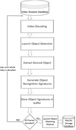
We present the approach behind our video analysis system in this sec-tion. Each video stream is first decoded to extract individual video frames. The objects of interest are extracted from the video frames by detecting and cropping around the area of detection. The local patterns of each extracted object are then generated and stored in the associated bu↵er. Object match-ing is then performed on the generated local features. The generated results are then stored in the database. Algorithm 1 shows the approach used in our object classification system.
The system applies multiple machine learning algorithms for detection and recognition in a cascaded way. The algorithms are employed in such a way that the results produced by one algorithm are further processed by the following algorithm. The first algorithm is used to extract the object of interest from the whole frame in such a way that it narrows down the image area. The rest of the frame which contains unwanted information is discarded to save processing time and resources. This algorithm independently operates on all the frames in a sequence. This results in the extraction of all the desired objects from all the video frames. Figure 1 presents the process followed in our approach.
Figure 1: Video Processing Workflow
3.1. Object Detection
We have used Haar Cascade Classifier for the extraction of objects – which involves extraction of “Haar” features from the image. Haar features are generated by computing the sum of pixels under the white rectangle region subtracted by the sum of pixels under the black rectangle region. These regions are adjacent to each other and possess the same shape and size. The integral images are helpful to compute the features very rapidly. The integral image can be computed by adding all the pixels above and to the left of a specific location [19]. Then by using four array references any rectangular sum can be calculated as:
I(x, y) = X
x0<x,y0<y
i(x0, y0) (1)
number of features generated by Haar is quite large, it is necessary to select features to reduce the dimensionality of the problem. This dimension reduc-tion can be best by using AdaBoost [20] – a learning algorithm which works in a cyclic process. It starts by keeping a set of weights which are distributed uniformly over every training example. It then selects one feature in its first cycle that gives best recognition performance and defines a weak classifier against it. The subsequent cycles assign higher weights to the training ex-amples that were misclassified by the first weak classifier. This enables the newly chosen feature to concentrate more on misclassified examples. This process continues and ultimately ends upon a strong classifier which is a lin-ear combination of all the weak classifiers selected during each cycle. Other approaches could also be used in this context, primarily focusing on the use of other bagging and boosting/ensemble-based learning approaches. A weak classifier hj(x) can be represented as [8];
h(x) =
⇢
1 pjfj(x)< pj✓j
0 Otherwise (2)
where fj(x) is the feature, ✓j is the threshold and pj is the parity to show
the direction of the inequality sign. For instance, consider an image that has the desired object (e.g. a face) and other regions which do not. By passing the image through a cascade of classifiers, it is possible to identify part of the image that is of interest. Continuing the example, as most of the image being considered is not likely to contain the desired object, the part of the image that passes the classifier will be the face region. This assumes that there is only one object of interest in the image being considered.
The extraction of desired objects from the frames helps to improve the performance of the system in two ways: (i) since the frame area is reduced so the analysis algorithm now has to process a smaller sized frame as compared to original one. This reduces the processing time of individual frame and in turn reduces the overall processing time of whole video. (ii) as the frame has been narrowed down to only object(s) of interest, by removing the unwanted area of the frame, it now contains only the desired object. The illumination e↵ects and noise which have the possibility to be present in the unwanted area is now taken care of. Since the unwanted areas are cropped out from the frame, these illumination e↵ects and noise will not reflect in the object recognition process. This will lead to improvement in the accuracy of overall system.
3.2. Object Classification
The extracted objects are then processed via the object recognition phase, which generates local binary patterns of all the extracted objects. These local binary patterns serve as features which can be used for the recognition of a known object. These features represent the extracted objects in such a way that they become highly discriminative and invariant to various gray-level changes in the objects.
We have used LBPH algorithm [9] for the generation of local pattern features. The algorithm makes use of the local binary patterns in order to generate feature vectors. LBP features (Algorithm 2) are computed by dividing the examined window into cells. Each cell contains a number of pixels. Then each pixel in the cell is compared to its neighboring pixels. If the value of center pixel is greater than its neighbour pixel, 1 is stored at that location. If it is the other way round then 0 is stored at that location. This is known as the labeling of pixels. LBP code of a single pixel of an image can be given as [9]:
LBPP,R= p 1 X p=0 s(gp gc)⇥2p (3) s(x) = ⇢ 1, x 0 0 x <0
gp = Neighbor Pixel ; gc = Centre Pixel
A histogram is then calculated and normalized for each occurrence. These normalized histograms give a feature vector of the window. The histogram is calculated as [9]:
H =X
x,y
Inf(x, y) =io, i = 0,1,2,3, ..., n 1 (4) where f(x,y) is the labeled image and n represents the labels which are gen-erated by the LBP operator.
The computation of the local pattern features is a compute intensive procedure as it involves the manipulation of every pixel in the video frame. The porting of this compute intensive procedure to GPUs is performed to reduce the computation demands. A GPU kernel (Algorithm 3) is developed for this purpose. It performs the procedure of local pattern feature generation in parallel instead of sequential processing as in a CPU.
Algorithm 2 Computing LBP on CPU
1: procedureComputeLBP
2: FrameHeight number of rows
3: FrameWidth number ofcolumns
4: for i++;i<FrameHeightdo 5: for j++;j<FrameWidthdo 6: gc[i][j] CentrePixel 7: gp[i][j] NeighbourPixel 8: if gp[i][j] gc[i][j]>0then 9: gp[i][j] 1 10: else 11: gp[i][j] 0 12: F rameData[i][j] p P i=1 N eighbourP ixels[i][j]⇤2p 13: Replace f rameData
In order to perform face recognition, the face image is divided into mul-tiple blocks or regions. Then for each block or region, LBP histogram is
Algorithm 3 Compute LBP on GPU
1: procedureKernel
2: c get current column
3: r get currentrow
4: idx get current pixel index
5: if c < F rameW idth ANDr < F rameHeight then
6: gc CentrePixel[idx] 7: gp NeighbourPixel[idx] 8: if gp gc >0 then 9: gp 1 10: else 11: gc 0
return F rameData[idx]
p P i=1
N eighbourP ixels[idx]⇤2p
12: Copy Back to Host f rameData
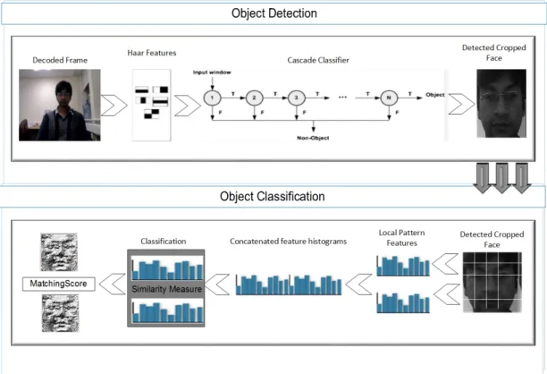
Figure 2: Object Detection and Classification Process
computed as explained above. The feature vector of the whole image is a combination of all LBP histograms of all regions in an image. Figure 2 shows the relation between Haar Cascade Classifier and the LBPH algorithm.
An object matching algorithm (Algorithm 4) is then applied on the lo-cal patterns of detected objects for recognition. The recognition process is performed by comparing the detected object features with the stored object information. The comparison is made on the basis of histogram intersec-tion which is used as a distance measure. The histogram intersecintersec-tion can be calculated as [21]: D(S, M) = B X b 1 min(Sb, Mb) (5)
Each comparison generates a score of each individual. These scores ob-tained after performing the histogram intersection determine the recognition
of marked person. We have used a threshold of 90 percent match in our experiments. We obtained over 90 percent accuracy rate in case of match-ing individual objects. The matchmatch-ing scores for unmatched individuals is 70 percent or below. The matching scores along with locations and time of presence are stored in the database. This module is totally unsupervised and is independent of any metric learning stage. The recognition is performed only on the basis of similarity measure between the features of two objects. Manually trained classifier is not required for this purpose.
Algorithm 4 Object Matching
1: procedureObjectMatching
2: LBPMarkedObjectHistogram LBP Histogram of Marked Object
3: LBPStreamObjectsHistograms LBP Histograms of Objects in Video Streams
4: for i++;i<LBPStreamObjectsHistograms do 5: MarkedObjectHistogram LBPMarkedObject 6: StreamObjectHistogram LBPStreamObjects[i] 7: HistogramIntersectionResult MarkedObjectHistogram \ StreamObjectHistogram 8: if IntersectionResult>0.9 then 9: ObjectFound 10: else 11: ObjectNotFound 4. System Architecture
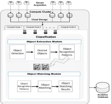
The overall architecture of the system is illustrated in Figure 3. The proposed system provides scalable and automated classification of objects in a large number of video streams in an unsupervised way. It is independent of the need of labelled training data and metric learning stage. The use of GPU enabled cloud compute nodes enables the system to achieve high throughput. Scalability challenge is also addressed by leveraging the benefits of GPU mounted servers in the cloud. The transfer time overhead of moving the video data from the camera to cloud storage is not considered in this work. This overhead is dependent on the speed of the network connecting the camera/data capture source to the cloud system.
The video streams are first fetched from cloud storage and are decoded to extract individual video frames. The decoded individual video frames
Figure 3: System Architecture
are stored in the input frame bu↵er. This bu↵er is a temporary storage in main memory for decoded video frames. The recorded video streams are encoded with the H.264 encoder to save storage space. Each video stream is recorded at 25 frames per second – with 3000 (120*25) video frames for a video stream of 120 seconds length. The number of decoded video frames is dependent upon the length of video stream being analyzed.
Each frame is then processed individually for object detection and recog-nition. The machine learning algorithms are applied on each frame for de-tection and recognition purposes. The objects of interest are first detected using the Haar cascade classifier algorithm. This detection helps to extract only the desired objects from the overall frame. The extracted objects are stored in the memory bu↵er for further processing.
The object extraction module mainly consists of object detection and cropping of detected objects. The object detection module searches the whole frame and provides detection of the objects of interest. Nothing is detected if an object of interest is not present in the frame. The video frame is then cropped around the detected object area. The cropping process removes the image areas that do not contain the desired objects and reduces the
operational area for the subsequent algorithm.
The next module after the extraction of desired objects is feature genera-tion module. This module generates the local patterns against each detected object. These local patterns serve as features which are further used to rec-ognize the marked object. This module mainly consists of the execution of local binary pattern histogram. A histogram of each of the detected objects is created and stored in the bu↵er as an output of this module. We have used a profiling mechanism to identify the compute intensive steps of our system. The generation of local pattern features is a compute intensive process. This compute intensive feature generation process has been ported to a GPU – through the design/ implementation of a kernel which performs generation of local patterns on GPUs. Each pixel of the video frame is mapped to a thread. This thread is then responsible for launching kernel for each pixel and processing it in parallel. The size of the thread block is dependent on the size of the frame. These threads work in a synchronous way to process frame data in parallel. A high level of parallelism is achieved since each pixel in the video frame is processed in parallel. Once the processing of frame bu↵er is completed, the resulting processed frame is stored in an output bu↵er – another temporary bu↵er in memory.
5. System Implementation
This section provides a description of the system components, their func-tionality and implementation. The operations employed to process video streams to support object detection and recognition are also described. 5.1. Video Decoding
The video streams are decoded to extract individual video frames – a total of 3000 frames for a video stream of 120 seconds length. These frames are then transferred to the processing module to enable the detection and recognition process to be carried out. Hence, each frame can be processed independently of each other. This approach enables the processing of indi-vidual frames on cloud resources, leading to high throughput and scalability. 5.2. Object Extraction
After the frame is decoded from the video stream, the next step is to extract faces from frames using an object detection algorithm. We have used Haar Cascade Classifier for this purpose. The input image is cropped around
Figure 4: Extracted faces from video streams
the output of Haar Cascade algorithm for the next step i.e. faces recognition. This helps to narrow down the area of image to a small rectangle containing the desired face. Figure 4 shows some of the extracted faces from the video streams. We also monitor the persistence of an object across multiple frames of a video stream. In this way, although each frame is individiually processed, tracking an object across multiple frames enables us to monitor its presence over a particular time period.
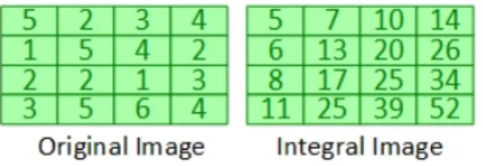
The Haar Cascade Classifier is constructed on top of Haar features which are extracted from objects present in video frames. In order to make the classifier scale-invariant, frame pyramid approach [22] has been used. The pyramid represents the same frame in multiple scales and enables the detector to be scale invariant. Objects with varying image sizes can easily be detected through the pyramid approach. An object pyramid can be constructed by using the down-sampling approach which samples the frame by one scale in each iteration. Integral image for each scale in the pyramid is then calcu-lated to speed up the process of generating a pixels sum. Integral image [19] helps to compute the summation of pixels present in a rectangular region by utilizing only four pixel corners. This approach of using integral images is highly efficient especially for the cases in which pixels sum of many rectan-gular regions of the same image need to be computed. Since the detector uses the sliding window approach and pixel sum for each shifted window is required, this approach reduces the complexity of the overall process. Figure 5 shows a representation of the integral image.
The sliding window is used, pixel by pixel, on the whole frame in search of a an object (e.g. a face). The area under the sliding window is passed to the cascaded classifier. As most of the image area is non-face region it groups the features into di↵erent stages based on the classifiers used. The region that passes all stages of the cascaded classifier is a face. The area under the sliding window is required to be passed through all stages of the cascade classifier. If at any stage, the input region is unable to pass the
Figure 5: Original and Integral Image
stage by not meeting the required threshold, it is immediately rejected. If the region passes all the stages successfully, then it is considered to be the face. On detection, an object recognition algorithm is invoked.
5.3. Local Feature Generation
Each detected object of interest is then analysed, by using local binary pattern histogram. The algorithm computes local binary patterns in order to generate feature vectors. In order to compute LBP features, the examined window is divided into multiple cells. Each cell contains a sub-block of 3⇥3 pixels. Then each pixel in the sub-block is compared to its neighboring pixels. If the value of centre pixel is greater than its neighbor pixel, 1 is stored at the location of that pixel. If the values of centre pixel is less than the neighboring pixel, the gray value of that pixel is replaced with 0. This makes the sub-block a binary block containing 0 and 1 depending upon its pixel values. This is known as the labeling of pixels. These labelled pixels generate a binary pattern which is then converted into one decimal value. The gray value of centre pixel is then replaced with the decimal value. This procedure is repeated on the whole image and an LBP image is obtained. A histogram is then calculated over the frequency of each number occurrence. This histogram gives a feature vector of the window.
In order to perform face recognition, the face image is divided into mul-tiple blocks or regions. Then for each block or region, LBP histogram is computed as explained above. The feature vector of the whole image is a combination of all LBP histograms of all regions in an image. Figure 6 shows the original faces and the LBP computed faces from video streams.
5.4. Similarity Measure
This procedure of LBP histogram generation is performed for all the video frames and the image which is to be matched. Matching is performed by comparing the LBP histogram of the marked object frame with all the
Figure 6: Original and LBP Faces
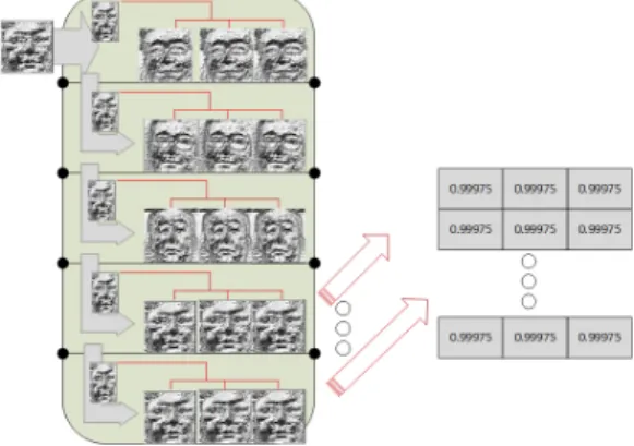
Figure 7: Visualization of matching process
frames of a video stream. The histogram intersection is used as a distance measure to calculate the similarity between two frames. After the persons face is authenticated correctly, the matching score associated to it is stored in a database. This phenomenon can be visualized in figure 7.
5.5. Local Pattern Feature Generation on GPUs
Generation of local patterns from a video frame is a compute intensive procedure. It is therefore ported to GPUs to reduce the computation de-mands. A GPU kernel is designed and implemented to perform this proce-dure. However, the execution flow is di↵erent which a↵ects the performance of the system. The processing of pixels is sequential in CPU based imple-mentation. A video frame with a width and height of 528⇥704 sequentially
can consume a lot of time (even for a single frame). The processing time increases exponentially when the number of video frames increases.
The GPU implementation on the other hand works in parallel fashion instead of sequential functionality like in a CPU. GPU implementation is known as GPU kernel and is executed by a number of threads generated by a GPU. The number of threads that a GPU can generate depends upon the processing cores of a GPU, memory and registers. It is also dependent upon the size of thread block and grid. Since each pixel is mapped to an individual thread, the number of generated threads should be equal to the number of pixels in a video frame. The availability of frame data in GPU memory enables the parallel processing of each pixel. Upon completion of the frame data processing, the processed frame data is copied back to CPU memory bu↵er (host) from GPU memory bu↵er (host).
We have used CUDA to implement and generate local pattern features on GPUs. It uses SIMD (Single Instruction Multiple Data) parallel program-ming model and provides a bunch of APIs to execute instructions on a GPU. A CUDA program initiates on a CPU and process data on a GPU through CUDA kernels. The GPU memory is first allocated, so that frame data can be transferred from CPU to GPU. The size of the GPU memory is allocated according to the size of video frame. Three di↵erent data transfer mecha-nisms including page-able memory, pinned memory and zero copy have been implemented and tested in this work. Upon successful completion of frame processing, the results are transferred back to the CPU memory.
The GPU kernel is executed by a number of threads. There can be a maximum of 32 threads in a warp and each thread block has numerous warps. Thread blocks are further grouped into grid. It is the responsibility of CUDA Work Distributor (CWD) to allocate thread blocks on a GPU. At the first step of kernel execution, these thread blocks are allocated. Kernal execution is performed in parallel with the help of CUDA streams.
The proposed system works partially on CPUs and partially on GPUs. The decoding of frames from video streams and extraction of faces is per-formed on a CPU. The compute intensive process of generation of local fea-tures is performed on a GPU using the CUDA kernel. The processed results are then transferred back to CPU. The results section provides a more de-tailed analysis of the accuracy of recognized objects and the processing time of the system.
6. Experimental Setup
This section provides the details of our experimental setup used to eval-uate the proposed system. The parameters used to evaleval-uate the perfor-mance of the system are the accuracy of the algorithms, processing speed-up achieved, resource consumption, scalability, and processing time of each video frame. The purpose of cloud based deployment is to evaluate the scalability of the system. The cloud deployment with GPUs evaluates the performance, throughput, resource consumption and processing time of video streams.
The configuration of the cloud resources is as follows: the cloud instance has Ubuntu LTS 14.04.1 and is running OpenStack Icehouse. There are six server machines and each server machine is equipped with 12 cores. Each server is running with 6-core Intel Xeon Processors at 2.4 Ghz. It has a storage capacity of 2 Terabyte with 32GB RAM. The cloud instance is con-figured with 192GB RAM, storage capacity of 12TB and 72 processing cores. OpenStack facilitates with a dashboard to manage and control the resources such as storage, network and pool of computers.
A cluster consisting of 15 nodes is configured to evaluate the proposed system. The configuration of each node is as follows: 4 VCPU running at 2.4GHz with 8GB RAM. Each node is configured with a storage capacity of 100GB. The evaluation parameters to measure the performance of the system include total analysis time of the system, impact of task parallelism on each node and the variations of compute nodes in the cloud. This experimental setup helps to measure the performance of the system for scalability and robustness with varying cloud configurations.
The Hadoop MapReduce framework is utilized to evaluate the system in cloud resources. Hadoop comes with Yarn which is responsible for man-aging resources and scheduling jobs for the running processes. It further facilitates with a NameNode in charge for the management of nodes, a Data/ComputeNode to process and store the data, and a JobTracker for the tracking of running jobs. These components of Hadoop MapReduce frame-work help to schedule and analyze tasks on the available nodes in parallel.
The accuracy and performance of the proposed system is evaluated on cloud nodes with 2 GPUs. The nodes are equipped with Intel Core i7 3.60 GHz processor with 16 GB RAM. Each node is supported with an ASUS GeForce GTX 780 GPU. This Kepler architecture based GPU is enriched with 12 Streaming Microprocessors (SM). It has 2304 CUDA cores and a memory of 3 GB. A total of 2048 threads can be generated in parallel by
each streaming processor. These threads are executed in 64 warps and each warp has the capability to execute 32 threads in parallel. A local memory of 512 KB is possessed by each thread and there are 255 registers per thread. Each streaming microprocessor (SM) uses 16 thread blocks with 2048 bytes of shared memory per block.
The GT610 GPU has 48 CUDA cores with a memory of 1GB. The archi-tecture of this GPU is Fermi based and has one streaming microprocessor. The streaming microprocessor can support a total of 8 thread blocks. It can support 48 warps per SM and each warp contains 32 threads. Each thread has a total of 63 registers and a local memory of 512kb.
The dataset is self-generated consisting videos of di↵erent objects. The total video data used for the experimentations consists of one month of video streams. Each video stream has a duration of 120 seconds. The video streams are encoded with H.264 format. The frame rate for each video stream is 25fps. The data rate and bitrate for each video stream are 421kbps and 461kbps respectively. The decoding of each video stream generates a frame set of 3000 video frames. Each video frame holds a data size of 371kb.
7. Experimental Results
This section explains the results obtained by executing the experiments with the dataset and the experimental setup with two di↵erent configurations mentioned in Section 6. This section is further divided into three subsections. The first subsection explains the accuracy of object classification system and the speedup achieved by the cropping process. The second subsection ex-plains the throughput and performance of the system for video stream de-coding, transfer of data between CPU to GPU and vice versa and perfor-mance gains achieved by utilizing the GPUs for compute intensive parts of the algorithm. The third subsection explains the scalability and robustness of the whole system by analyzing decoded video streams and transferring the video data from local storage to cloud nodes. It also measures the time required to analyze video data on the cloud nodes and gathering the results after the completion of analysis. A discussion of the observations from these results is also provided in this section.
7.1. Performance of the unsupervised object classification
The performance of the unsupervised object classification system is evalu-ated by measuring the accuracy to classify objects and the speedup achieved
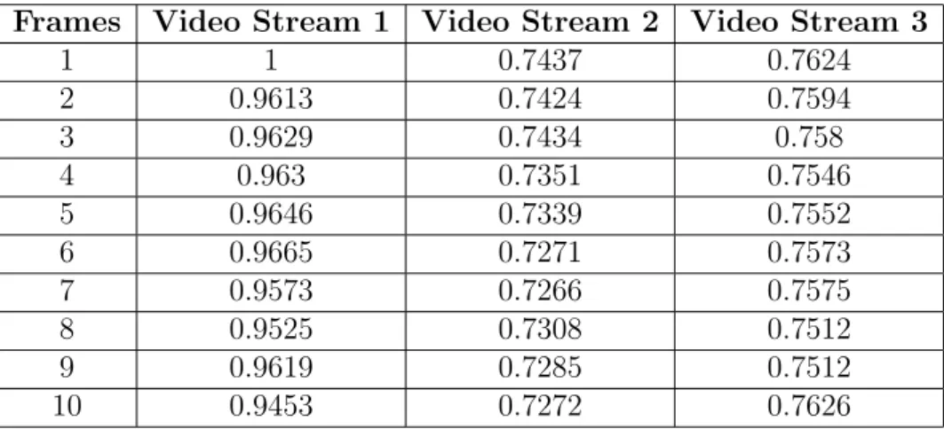
Frames Video Stream 1 Video Stream 2 Video Stream 3 1 1 0.7437 0.7624 2 0.9613 0.7424 0.7594 3 0.9629 0.7434 0.758 4 0.963 0.7351 0.7546 5 0.9646 0.7339 0.7552 6 0.9665 0.7271 0.7573 7 0.9573 0.7266 0.7575 8 0.9525 0.7308 0.7512 9 0.9619 0.7285 0.7512 10 0.9453 0.7272 0.7626
Table 1: Matching results of a person in multiple video streams
by the cropping process.
7.1.1. Object Classification Accuracy
The marked object which is to be identified in the video stream is matched with all the frames of a video. It is to be noted that for a video stream with a frame per second rate of 25, we decoded only 5 frames per second. It is obvious that no change can occur in such a short interval of time, so processing all the frames would only increase the processing time. Table 1 shows the matching results of a marked object with multiple frames of multiple video streams.
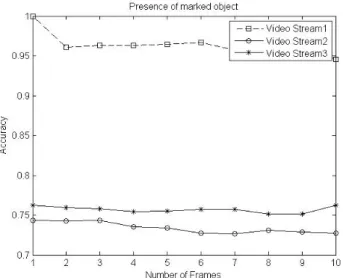
The values in the columns represent the distance measure of marked ob-ject against di↵erent objects of multiple video streams using the LBPH al-gorithm. The values near to 1 depict a closer match of marked object. It can be seen from the table that all values in the column of video stream 1 are above 90 percent. This shows that the marked object is present in the video stream 1. On the other hand, all values in the second and third video streams are below 90 percent and depict that the marked object is not present in these video streams. So we have used a threshold of 90 percent to distinguish between the matched and unmatched objects. Figure 8 shows the video streams in which the marked object is most likely to reside.
It can be seen from the figure that video stream 1 has the highest proba-bility of having the marked object. The other two streams are not probable to contain the marked object. Local binary pattern histogram hence provides
Figure 8: Presence of marked object in multiple streams
a good measure for the presence of marked objects in video streams.
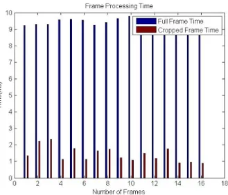
Cropped Frame Processing Time: A significant amount of speedup is achieved in the processing time of each frame due to the object detection approach. Cropping of video frame around the detected object helped to reduce the processing area for LBPH algorithm. The resolution of overall video frame is decreased which in turn reduced the overall processing time of frame. The processing time of each individual frame before cropping and after cropping is calculated and is shown in Figure 9.
The decrease in processing time is because of the fact that the resolution is reduced significantly because of cropping. The video used in this experiment had a frame resolution of 640⇥480. But the detected object which was extracted from the whole frame and later used by LBPH for comparison had a resolution of around 160⇥160 in most of the cases. This decrease in resolution improved the total frame processing time by almost 90%.
7.2. Object Classification on GPUs
This section describes the throughput and performance of the object clas-sification system. The analysis of object clasclas-sification system on GPU can be divided into two major steps i) time required for decoding a video stream and transferring it from CPU to GPU memory, ii) time required to process
Figure 9: Frame processing time of individual frames
the video frame data for object classification. The performance measures of these two major steps are explained in the rest of this subsection.
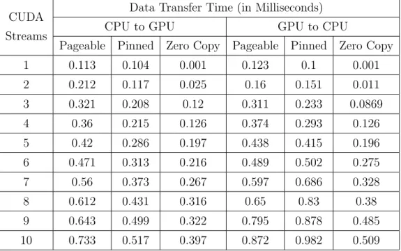
7.2.1. Data Transfer Time
We have tested three di↵erent memory allocation techniques to transfer data from CPU to GPU and then back from GPU to CPU. The three tech-niques are page-able memory, pinned memory and zero copy. The e↵ect of these three techniques has been demonstrated by varying the number of video streams from 1 to 10. A total memory allocation of 371.712 KBs is required by each video frame with a resolution of 704⇥528. A video stream recorded at 25 frames per second has a data transfer rate of 10.89 MB per second. For a varying number of video streams from 1 to 10, the data transfer per second varied from 10.89 MB to 108.9 MB. It has been observed that zero copy memory allocation technique remained fastest among the three tech-niques for transferring video frame data from CPU to GPU and vice versa. The time taken by each technique is summarized in Table 2.
7.2.2. Frame Processing Time
The total time taken to process an individual frame of a video stream is calculated by using the three memory allocation techniques discussed in the previous section. The total time required to process an individual video frame
CUDA Streams
Data Transfer Time (in Milliseconds)
CPU to GPU GPU to CPU
Pageable Pinned Zero Copy Pageable Pinned Zero Copy
1 0.113 0.104 0.001 0.123 0.1 0.001 2 0.212 0.117 0.025 0.16 0.151 0.011 3 0.321 0.208 0.12 0.311 0.233 0.0869 4 0.36 0.215 0.126 0.374 0.293 0.126 5 0.42 0.286 0.197 0.438 0.415 0.196 6 0.471 0.313 0.216 0.489 0.502 0.275 7 0.56 0.373 0.267 0.597 0.686 0.328 8 0.612 0.431 0.316 0.65 0.83 0.38 9 0.643 0.499 0.322 0.795 0.878 0.485 10 0.733 0.517 0.397 0.872 0.982 0.509
Table 2: Data Transfer Time from CPU to GPU and GPU to CPU
involves is the sum of time required to read and decode a frame, transfer time from CPU to GPU and GPU to CPU and the time required to compute local binary pattern of frame. The figure 10 depicts the elapsed time of di↵erent frame processing operations by each memory allocation technique. It has been observed that zero copy remained the most efficient mechanism because of direct video frame data access from GPU to CPU. GPU memory address space is mapped to CPU memory address space in zero copy mechanism, so GPU can access CPU memory as its own address space. This mapping also enables the GPU to access a particular memory location in host memory whenever data is copied from host to device. The same procedure is followed to copy data back to the host from GPU memory.
Another way to quantify the performance of the system is to measure the number of frames processed per second. The number of frames processed per second using the three memory allocation mechanisms is calculated and de-picted in figure 11. As it was predicted, the highest throughput is achieved by the zero copy mechanism with varying number of video streams. It is observed that two video streams per GPU provided the most optimum
per-Figure 10: Frame Processing Operations and Processing Time
formance by processing almost 100 frames per second. By increasing the number of video streams a steep reduction was observed in the frame pro-cessing time. This is because of the fact that data transfer time from CPU to GPU and GPU to CPU remained optimized with two CUDA streams as described in Table 2.
7.2.3. Computation Time with Varying Video Resolutions
The processing time of a video frame is highly dependent on the resolution of a video frame. For a high resolution video frame, more computation time is required as more data is needed to be processed. We have tested di↵erent video streams with varying resolutions on the system and computed the total processing time. This time includes the time required to process the frame as well as the video decoding time. The generated results are also compared with the results produced by stand-alone CPU node as depicted in figure 12. It has been observed that optimum utilization of GPUs can be achieved by having the videos with high resolution. The processing of low resolution videos on GPUs will not generate much speedup as compared to CPUs. This is because of the fact that a CPU processes each pixel sequentially. On the other hand a GPU performs the processing of pixels in parallel by mapping each pixel to individual thread. This elevates the processing speed of indi-vidual frames. However, if the video frame is of low resolution, no significant
1 2 3 4 5 6 7 8 9 10 0 20 40 60 80 100 120 140
Number of Video Streams
Frames Processing Per Second
Pageable Memory Pinned Memory Zero Copy
Figure 11: Frame processing time and number of Video Streams
256x144 352x240 480x360 640x480 704x528 1280x720 1920x1080 0 10 20 30 40 50 60 70 80 90 100
Varying Video Resolutions
Video Processing Time (s)
Stand−alone CPU node Cloud node with GT610 Cloud node with GTX 780
Figure 12: Video Processing comparison on di↵erent Platforms
speedup in the processing time of video frame is observed as compared to CPU due to data transfer overheads.
7.3. Object Classification on the Cloud
In order to evaluate the scalability of our approach, we have executed it on the cloud infrastructure described in the experimental setup section. The evaluation is performed on the following three parameters. i) Time taken to transfer video stream data from storage server to the cloud nodes ii) Analysis time of video streams on various cloud nodes iii) Time required to collect results from cloud nodes. Hadoop File System (HDFS) is utilized for storing files. The MapReduce framework is used to analyze video streams by
executing unsupervised object classification algorithm explained in Section 3. The analysis results are then stored in the database.
7.3.1. Hadoop Sequence File Creation
The video streams are first decoded to extract individual video frames from the input video. The total size of one month of recorded video streams is 175GB. Each video stream is recorded at 25 frames per second. The number of decoded video frames is dependent upon the length of video stream being analyzed. These individual frames are not suitable for directly processing on the compute nodes with the MapReduce framework. This is because of the fact that MapReduce is designed to process large files. Processing small files will only result in the decrease of overall performance. These small files are bundled into a large file termed as Hadoop sequence file and then transferred to the cloud nodes for processing. The sequence file is then moved to cloud storage for unsupervised object classification.
7.3.2. Hadoop Sequence File Creation Time
The time required to generate a sequence file is directly proportional to the size of dataset. Multiple datasets of varying sizes from 5GB to 175GB have been used in this paper to generate results. The dataset of varying sizes helped to evaluate numerous aspects of our system. The time taken to create a sequence file for sizes ranging from 5GB to 175GB varied from 6.15 minutes to 10.73 hours respectively. The larger the dataset, more time it will require to generate the sequence file. However, it is a one-time process and once the sequence file is generated, it can be stored in the cloud data storage for future analysis tasks.
7.3.3. Sequence File Transfer Time
The generated sequence file is moved to cloud data storage as object classification will be performed on cloud nodes for analysis. The transfer time required to transfer the file to cloud data storage depends on various parameters. These parameters include network bandwidth, data replication factor and cloud data storage block size. The data transfer time varies with the size of the dataset. For the dataset sizes reported in this paper (5GB to 175GB), the data transfer time varied from 2 minutes to 3.17 hours. Figure 13 depicts the data transfer time of various dataset sizes with varying cloud storage block size.
Figure 13: Data Transfer Time to Cloud Storage
Figure 14: Video Stream Analysis Time on Cloud Nodes
7.3.4. Object Classification on Cloud Nodes
We have evaluated the scalability and robustness of the system by exe-cuting object classification on large number of video streams. The datasets have also been varied from 5GB to 175GB to observe the e↵ects on the cloud nodes. The HDFS block sizes have also been varied to measure the execution time and resources consumed during the analysis tasks on cloud nodes. The performance of the system is measured by measuring the time required to analyze the dataset of various sizes and the resources consumed during the analysis task.
We have varied the block size from 64MB to 256MB, in order to observe the e↵ect of varying block size on Map task execution. It has been observed that the execution time of Map task increases by increasing the size of dataset as depicted in figure 14. But the variation in block sizes has no major impact on the execution time of Map/Reduce tasks. For the dataset size varying be-tween 5GB and 175GB, the total execution time varied bebe-tween 6.38 minutes and 5.83 hours.
The memory consumption of all the block sizes remained the same except for the 64MB block. The requirement of physical memory for the 64MB
Figure 15: Memory Consumed for Analysis in the Cloud
Nodes Tasks per Node Tasks Execution Time (Hours) 15 94 5.83 12 117 7.10 9 156 7.95 6 234 14.01 3 467 27.80
Table 3: Analysis Task Execution Time with Varying Cloud Nodes
block size is higher than other block sizes as depicted in figure 14. The default block size of cloud storage is 128MB. A 64MB block size thus produces more data blocks which are needed to be processed by cloud nodes causing memory overhead. More memory is required to process small block sizes as the number of map tasks turn out to be deficient with the smaller block sizes. Figure 15 shows the memory required with varying datasets for analysis on the cloud.
7.3.5. Robustness with changing cluster size
The robustness of the system is evaluated by measuring the total analysis time and the speedup achieved by increasing the number of cloud nodes. We have measured the total time required for the analysis of dataset with varying number of nodes. The total analysis time of whole dataset decreases as the number of nodes increases in the cloud. Table 3 shows the execution time required to analyze the dataset with varying nodes.
We have also measured the total time required for analysis of whole dataset with varying number of nodes and block sizes. Figure 16 depicts that
Figure 16: Analysis Time with Varying Number of Cloud Nodes
the execution time decreases as the number of nodes in the cloud increases. A decreasing trend has been observed in the analysis of whole dataset. A total execution time of 27.80 hours was required for the processing of 175 GB dataset with 3 nodes, whereas, it took only 5.83 hours to process the same amount of data with a 15 node cloud.
7.3.6. Task parallelism on Compute Nodes
The total number of analysis tasks executing on a compute node is di-rectly proportional to the number of input splits. The number of input splits are further dependent on the dataset size, cloud data storage block size and available physical resources. The dataset size of 175GB gives rise to 1400 map/reduce tasks with a default cloud storage block size of 128MB. It has been observed during the experiments that the number of analysis tasks on each node increases as the number of nodes decreases. We varied the number of nodes between 3 and 15 in these experiments. As the number of tasks per node increases, the performance of the overall system degrades. This is be-cause of the fact that the increase in number of tasks per node generates over occupied resources and each task has to wait more for scheduling and exe-cution. A summary of task execution time corresponding to varying number of nodes is shown in table 3.
We have also calculated the analysis time of varying datasets with varying block sizes. It is observed that if the block size is large, less computation time will be required to analyze the data as compared to smaller block size. The large block size will have less number of map tasks, reduced memory requirement and management overhead as compared to small block size. This will result in the faster processing of dataset. However, it is to be noted that varying block sizes does not a↵ect the execution time of Map task. The block size of 512MB required the same processing time as 256MB block size for the
175GB dataset. The same phenomenon is observed with other block sizes as well. However, the time required to transfer the data with larger block sizes is greater and required larger compute nodes to process the data.
The reducers in the map/reduce tasks have the responsibility to gather the analysis results and write them on the output sequence file. A separate utility is used to extract meta-data from the output sequence file. This contains the classification results obtained from the object classification approach.
8. Conclusion & Future Work
A cloud based video analysis system based on Haar Cascade Classifier and the Local Binary Pattern Histogram is presented in this paper. The proposed system requires minimum human interaction and provides auto-mated object classification from large number of video streams. The system performs classification under unsupervised learning domain and without re-quiring any metric learning stage or labelled training dataset. An accuracy of more than 95 percent is achieved when the application is tested on multi-ple video streams. Also a speedup of 90 percent is achieved to recognize an object on individual frame as compared to full frame.
The proposed system is capable of coping with the challenges of increased volume of data. The objects are detected and classified from one month of video data comprising a size of 175 GB. It took 6.52 hours to analyze this data on a 15 node cloud. By increasing the number of nodes in the cloud, a decreasing trend in processing time is observed in analyzing the video data. A reduction from 27.80 hours to 5.83 hours is observed, when the number of cloud nodes increased from 3 to 15. However, the analysis time is also dependent on the amount of data being analyzed. The analysis time varied from 6.38 minutes to 5.83 hours for the dataset sizes ranging from 5GB to 175GB in the cloud.
The processing time further reduced to 3 hours for 175GB data when the video stream analysis is performed on GPU mounted cloud nodes. Several factors contributed to achieving high throughput such as optimized resource utilization of GPUs, efficient and optimal data transfer techniques, improved occupancy and efficient memory allocation. The mapping of each pixel of a video frame to individual light-weight GPU threads played a major role in achieving high performance in the system.
In future, we would like to make the system more generic by detecting and recognizing other objects from di↵erent object classes such as cars, bikes
and pedestrians. The optimization of detection and recognition algorithms by analyzing them in the frequency domain will also be the focus of our future work. We would also like to achieve more speedup and scalability by using in-memory processing cluster coupled with the computation power of GPUs. This will help to overcome the delays which occur due to various I/O operations.
References
[1] L. Zhang, M. Yang and X. Feng, Sparse representation or collaborative representation: Which helps face recognition, IEEE International Con-ference on Computer Vision, pp. 471478, 2011.
[2] X. Zhu and D. Ramanan, ”Face detection, pose estimation, and landmark localization in the wild, IEEE International Conference on Computer Vi-sion and Pattern Recognition, pp. 28792886, 2012.
[3] H. Cevikalp, B. Triggs and V. Franc, Face and landmark detection by using cascade of classifiers, IEEE International Conference on Face and Gesture Recognition, pp. 17, 2013.
[4] J. S. Bae and T. L. Song, Image tracking algorithm using template match-ing and PSNF-m, International Journal of Control, Automation and Sys-tems, vol. 6, pp. 413-423, 2008.
[5] Project BESAFE (Behavior lEarning in Surveilled Areas with Feature Extraction), http://imagelab.ing.unimore.it/besafe/, Last accessed: 20-02-2016
[6] A. Jain, B. Klare and U. Park, Face recognition: Some challenges in forensics IEEE International Conference on Automatic Face and Gesture Recognition and Workshops, 2011.
[7] Y. Taigman, M. Yang and L. Wolf, ”DeepFace: Closing the gap to human-level performance in face verification, IEEE Conference on Computer Vi-sion and Pattern Recognition, pp.1701-1708, 2014.
[8] H. Wang, X. Gu, X. Li and Z.Li, Occluded face detection based on ad-aboost technology, IEEE Eighth International Conference on Internet Computing for Science and Engineering, pp. 8790, 2015.
[9] A. Suruliandi, K. Meena, and R. Reena, Local binary patterns and its derivatives for face recognition. IET Computer Vision, pp. 480-488, 2012. [10] R. Lienhart, L. Liang, and A. Kuranov, A detector tree of boosted classi-fiers for real-time object detection and tracking, International Conference on Multimedia and Expo, pp. 27780, 2003.
[11] Y. Lin, F. Lv, S. Zhu, M.Yang and L.Cao. Large-scale Image Classifi-cation: Fast Feature Extraction and SVM Training. IEEE Internatioanl Conference on Computer Vision and Pattern Recognition, pp. 1689-1696, 2011.
[12] V. B. Nikam and B. B. Meshram, Parallel and Scalable Rules Based Classifier using Map-Reduce Paradigm on Hadoop Cloud. International Journal of Advanced Technology in Engineering and Science, vol.2, pp.558-568, 2014.
[13] G. H. Nguyen, S. L. Phung and A. Bouzerdoum, Reduced Training of Convolutional Neural Networks for Pedestrian Detection. The 6th Inter-national Conference on Information Technology and Applications, pp. 61-66, 2009
[14] H. Tan and L. Chen, An Approach for Fast and Parallel Video Pro-cessing on Apache Hadoop Clusters. IEEE International Conference on Multimedia and Expo, pp. 1-6, 2014.
[15] X. Tang, Z. Ou, T. Su and P. Zhao, Cascade AdaBoost Classifiers with Stage Features Optimization for Cellular Phone Embedded Face Detec-tion System, Advances in Natural ComputaDetec-tion, vol 3612, pp. 688-697, 2005.
[16] B. Zhou, W. Wang and X. Zhang, Training Backpropagation Neural Network in MapReduce, International Conference on Computer, Com-munications and Information Technology, pp. 22-25, 2014.
[17] C. Rosenberg, M. Hebert and H. Schneiderman, Semi-Supervised Self-Training of Object Detection Models. IEEE International Conference on Application of Computer Vision. 2014.
[18] B. Pfahringer, G. Holmes and E. Frank Classifier chains for multi-label classification, Machine Learning Springer, pp. 333 359, 2011.
[19] T. Wu and A. Toet, Speed-up template matching through integral image based weak classifiers, Journal of Pattern Recognition Research, Volume 12, 2014.
[20] T. Wu and A. Toet, Speed-up template matching through integral im-age based weak classifiers, Journal of Pattern Recognition Research, pp. 192199, 2014.
[21] G. Sharma and F. Jurie ”A novel approach for efficient SVM classifica-tion with histogram intersecclassifica-tion kernel,” British Machine Vision Confer-ence, 2013.
[22] D. Nguyen Ta, W. Chen, N. Gelfand and K. Pulli, ”SURFTrac: Efficient tracking and continuous object recognition using local feature descrip-tors,” IEEE Conference on Computer Vision and Pattern Recognition, pp.2937-2944, June 2009.
[23] Y. Wu, C. Wu, B. Li and F. Lau, CloudMedia: When cloud on demand meets video on demand, 31st international conference on Distributed Computing Systems, pp. 268-277, 2011
[24] W. Wang, W. Zhang, F. Gong, P. Zhang and Y. Rao, Towards a Perva-sive Cloud Computing based Food Image Recognition, IEEE international conference on Cyber, Physical and Social Computing, pp.2243-2244, 2013 [25] J. Fan, F. Han and H. Liu, Challenges of Big Data Analysis, National
Science Review, pp 293-314, 2013
[26] K. Wiley, A. Connolly, S. Krugho↵ and B.Howe, Astronomical Data Analysis Software and Systems, p.93, 2011
[27] L. Zhu, X. Zheng, P. Li and Y. Wang, A Cloud Based Object Recognition Platform for IOS, International Conference on Identification, Information and Knowledge in the Internet of Things, pp. 68-71, 2014
[28] R. Raina, A. Madhavan and A. Y. Ng, Large scale deep unsupervised learning using graphics processors, 26th ACM Annual International Con-ference in Machine Learning, pp. 873-880, 2009
[29] W. Wang, Y. Zhang, S. Yan and H. Jia, Parallelization and performance optimization on face detection algorithm with OpenCL: A Case Study, Tsinghua Science and Technology, vol. 17, no. 3, pp 287-295, 2012
[30] Z. Jing, J. liangbao and C. Xuehong, Implementation of parallel full search algorithm for motion estimation on multi-core processors, IEEE 2nd International Conference on Next Generation Information Technol-ogy, pp 31-35, 2011
[31] A. Mohamed, G. Dahl and G. Hinton, Acousting modeling using deep belief networks, IEEE Transactions on Audio, Speech and Language Pro-cessing, vol. 20, issue 1, pp. 14-22, 2011
[32] S. Gao, I. Tsang and L. Chia, Laplacian sparse coding, hypergraph laplacian sparse coding and applications , IEEE Transactions on Pattern Analysis and Machine Intelligence, pp. 92-104, 2012
[33] D. oro, C. Fernandez, J.R. Saeta, X. Martorell and J. Hernando,Real time GPU based face detection in HD video sequences, IEEE Interna-tional Conference on Computer Vision Workshops, pp. 530-537, 2011 [34] A. Anjum, T. Abdullah, M. F. Tariq, Y. Baltaci and N. Antonopoulos,
”Video Stream Analysis in Clouds: An Object Detection and Classifica-tion Framework for High Performance Video Analytics”, IEEE Transac-tions on Cloud Computing, pp. 1-14, 2015