Adaptive Step Length Selection in Gradient Boosting for Generalized Additive Models for Location, Scale and Shape

(1)

Adaptive Step Length Selection in

Gradient Boosting for Generalized

Additive Models for Location, Scale

and Shape

Boyao Zhang

Supervisor: Prof. Dr. Sonja Greven

Co-Supervisor: Dr. Elisabeth Waldmann

Tobias Hepp

Master Thesis

Institut f¨

ur Statistik

Ludwig–Maximilians–Universit¨

at M¨

unchen

Munich, May 1, 2019

(2)

Abstract

Generalized additive models for location, scale and shape (GAMLSS) are an approach that regresses not only the expected mean value as the conventional generalized additive models but also other distribution parameters. Fitting the GAMLSS with boosting algo-rithm allows simultaneous estimation of predictor effects and variable selection. The non-cyclical componentwise gradient boosting approach reduces the optimizing procedure from a multi-dimensional to a one-dimensional problem with vastly decreased complexity. Tun-ing in boostTun-ing algorithm relies mainly on the number of iterations of the algorithm. The other flexible component step length in most cases is set to 0.1. When developing complex models like GAMLSS, this setting will lead to unbalanced decisions. This thesis studied the influence of the adaptive step length on this balance and other performance measures.

Based on the simulation study, the adaptive approach usually updates the distribution parameters in a balanced manner. Within the limited number of boosting iterations, the adaptive approach will also lead to better estimations than the fixed step length settings, especially when the coefficients are huge. When fitting the high dimensional data, the adap-tive approach is more efficient in computing. This thesis also introduced a semi-analytical adaptive step length (SAASL) algorithm for the Gaussian distribution, which is faster and more stable in balance than the adaptive step length found by doing a line search. Based on the mathematical induction, the optimal step length of the scale parameter in Gaussian distribution converges to 0.5. Applying this step length to the SAASL will result in a much more faster algorithm (SAASL05) at the cost of slightly unbalanced decisions. Because of the aggressive step length in each iterations, the adaptive approaches cannot good estimated the correlated models.

Keywords—GAMLSS, gradient boosting, componentwise gradient boosting, adaptive step length, semi-analytical adaptive step length

(3)

Acknowledgement

Firstly, I would like to express my sincere gratitude to my supervisor Prof. Dr. Sonja Greven for her support of my thesis for her patience, motivation and immense knowledge. Her advice gave me a lot of inspiration.

Besides my supervisor, I would like to acknowledge Dr. Elisabeth Waldmann and M.Sc. Tobias Hepp, Faculty of Medicine, Friedrich-Alexander-Universit¨at Erlangen-N¨urnberg. They listened to my ideas patiently and directed me with lots of valuable advice.

I would like to thank Dr. David Rügamer, Department of Statistics, Ludwig-Maximilians-Universität München for his encouragement and help.

I would also like to thank my friends Miao Liu and Yingxin Cai for their support and en-couragement. They make my life more colourful.

Finally, I must express very profound gratitude to my parents and my grandma for providing me with unfailing support and continuous encouragement throughout my years of study and through the process of researching and writing this thesis.

(4)

List of Algorithms

1 Forward Stagewise Additive Modeling . . . 7

2 Gradient Boosting Algorithm . . . 8

3 Componentwise Gradient Boosting . . . 10

4 Cyclical componentwise gradient boosting in multiple dimensions . . . 15

5 Non-cyclical componentwise gradient boosting in multiple dimensions . . . 17

6 Golden Section Search . . . 21

7 Non-cyclical componentwise gradient boosting in Gaussian distribution with dif-ferent step lengths . . . 28

(7)

LIST OF FIGURES

List of Figures

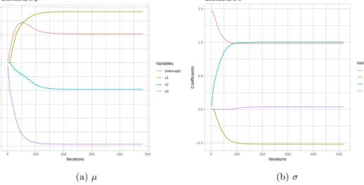
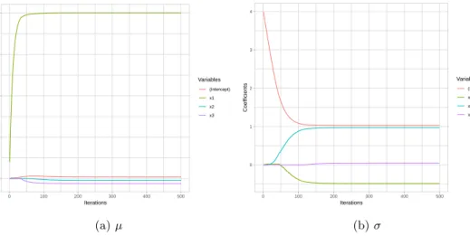
1 Estimated coefficients ofµandσin each iterations . . . 33

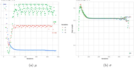
2 Step length ofµandσ in each iterations . . . 34

3 Comparison of the ASL and SAASL . . . 35

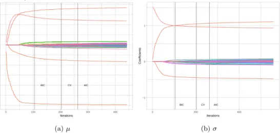
4 Demonstration of early stopping . . . 36

5 Demonstration of early stopping method on coefficients plot . . . 36

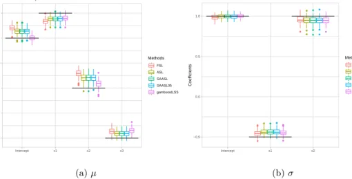
6 Comparison: Estimated coefficients . . . 38

7 Comparison: Mean Squared Error (MSE) . . . 39

8 Comparison: Empirical risk . . . 39

9 Demonstration of unbalanced decisions . . . 41

10 Demonstration of balanced decisions . . . 41

11 Comparison: Balance of decisions . . . 42

12 Comparison: mstop . . . 43

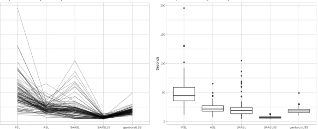
13 Comparison: Computing time . . . 44

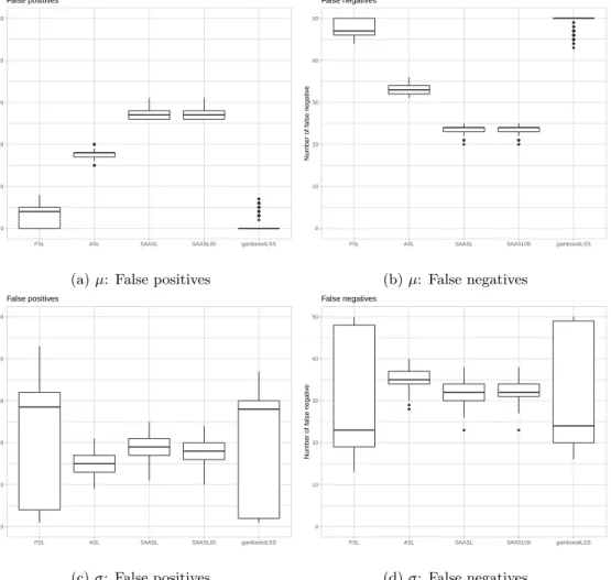
14 Comparison: False positives & False negatives I . . . 46

15 Comparison: False positives & False negatives II . . . 47

16 Coefficients and adaptive step length of GAM . . . 49

17 Harmonic mean . . . 50

B.1 Slope ofµandσover iterations . . . 63

B.2 Negative log-likelihood over iterations . . . 63

B.3 mstop of Comparison False positives/negatives II . . . 64

B.4 Comparison: Estimated coefficients ofµ . . . 65

B.5 Comparison: Estimated coefficients ofµ . . . 65

B.6 Comparison: Estimated coefficients ofσ . . . 66

B.7 Comparison: Estimated coefficients ofσ . . . 66

B.8 Comparison: Mean Squared Error (MSE) of µ. . . 67

B.9 Comparison: Mean Squared Error (MSE) of µ. . . 67

B.10 Comparison: Empirical risk . . . 68

B.11 Comparison: Empirical risk . . . 68

B.12 Comparison: Balance of decisions . . . 69

B.13 Comparison: Balance of decisions . . . 69

B.14 Comparison: mstop . . . 70

B.15 Comparison: mstop . . . 70

B.16 Comparison: Computing time . . . 72

B.17 Comparison: Computing time . . . 74

B.18 Comparison: False positives & False negatives of µ . . . 76

B.19 Comparison: False positives & False negatives of σ . . . 78

B.20 Comparison: False positives & False negatives of µ . . . 80

(8)

1. INTRODUCTION

1

Introduction

The generalized additive models for location, scale and shape (GAMLSS) were introduced by [Rigby and Stasinopoulos, 2005], which regress the univariate response with a set of statistical models. It is a more generalized model of the conventional generalized additive models (GAM) [Hasties and Tibshirani, 1990], as the latter regress only the location parameter. Given a set of covariates, the GAMLSS do not require the conditional distribution of the response variable to be a member of the exponential family. The optional distributions for GAMLSS can be found from the work of [Stasinopoulos and Rigby, 2007]. Another feature of GAMLSS is that every distribution parameter is modelled by its own predictor and an associated link function [Mayr et al., 2012]. The estimation of the coefficients is usually based on the penalized maximum likelihood [Rigby and Stasinopoulos, 2005]. Just like the other common used regression models (e.g. linear model or GAMs), the variable selection is an important procedure, especially for the high dimensional data. The generalized Akaike information criterion (GAIC) can be used as a selection method [Rigby and Stasinopoulos, 2005], but this procedure is infeasible when there are more covariates than observations [Mayr et al., 2012]. Moreover, other shortcomings like the inclusion of a large number of non-informative variables [Ripley, 2004] are also inherited by the GAIC. Some authors [B¨uhlmann and Yu, 2003] showed that the gradient boosting can be applied to fit the generalized additive models, and they also found that the variable selection procedure is included in the modified algorithm, i.e. the componentwise gradient boosting algorithm, which updates only one predictor in each iteration. This approach was also generalized to the GAMLSS models (denoted asgamboostLSS) [Mayr et al., 2012], which performs the estimation and variable selection simultaneously. The original gamboostLSS algorithm is a “cyclical” fitting, i.e. every distribution parameters of the univariate response variable will be updated in each iteration. As the gradient boosting an algorithm that tends to select a relatively high number of false-positive variables, some authors [Thomas et al., 2018] introduced a “non-cyclical” fitting that combines the gamboostLSS with the stability selection [Meinshausen and B¨uhlmann, 2010], which is a generic method that investigates the importance of the covariates in a statistical model by repeatedly subsampling the data. By this way, not only the variable selection, but also a selection of the best submodel (location, scale, or shape) that leads to the largest improvement in model fit is also performed in the “non-cyclical” approach. Moreover, the maximum number of boosting iterations for each distribution parameter can be replaced with the overall number of iterations. Thus tuning the complete model reduces from a multi-dimensional to a one-dimensional optimization problem. The computing time, hence, reduced drastically.

In contrast with the “cyclical” algorithm, the “non-cyclical” fitting, however, destroyed the internal balance between the distribution parameters. In other words, some parameters will be updated more frequently than the others. If the cost of large numbers of iteration can be ignored, this unbalanced decisions will not affect the final estimations, as all distribution parameters can be fitted sufficiently. But if the maximum of the number of boosting iteration is limited, those parameters whose potential improvement are intrinsically small will get little chance to be updated.

(9)

1. INTRODUCTION

A possible solution to the unbalanced decision is using the adaptive step length to update the predictor in each iteration, i.e. finding the optimal step length based on the reduction of the empirical risk, and use it to update the base-learners. By this way, the predictors of distribution parameters with a vast improvement in each iteration can be updated rapidly. Thus, the balance of decision is kept, because the remaining improvement of these predictors and the potential improvement of the other parameters, whose values are intrinsically small, are on the same level.

The idea of using the adaptive step length in gradient boosting was introduced by [Friedman, 2001], whose value in each iteration is estimated by performing a line search. However, the step length in most cases is set to 0.1, because some authors [B¨uhlmann and Hothorn, 2007] argued that the use of this adaptive step length is unnecessary, as the procedure of doing a line search costs additional computing time. Nearly all publications accepted this setting and study mainly the number of iterations of the algorithm or its practical applications. Nothing has been published that study the influence of the step length on the balance of decisions in GAMLSS models.

This thesis studied the effect of the step length on this balance and compared the perfor-mance of the estimation between the adaptive step length and the fixed step length (set with 0.1). Accounting for the additional runtime of the line search, we also introduced a semi-analytical method (SAASL) to determining the adaptive step length in Gaussian distribution, which com-putes the adaptive step length analytically instead of an optimizing procedure. As the analytical solution to the scale parameter in Gaussian distribution does not exits, we replace its optimal step length in each iteration with a constant asymptotic value (0.05), which is even though not an adaptive value but a more reasonable and appropriate value. So we get a new algorithm (SAASL05), which quits the optimizing procedure and result in a more faster algorithm with almost little costs.

This thesis is organized as follows: In section 2 we describe briefly the generalized additive models for location, scale and thape (GAMLSS). The theory of generalized additive models for location, scale and shape (GAMLSS) is introduced in section 3. Section 4 demonstrated the boosted GAMLSS and listed the “cyclical” and “non-cyclical” componentwise gradient boosting algorithms for GAMLSS. Section 5 describes the step length in gradient boosting, including the effectiveness of fixed step length, the line search method used in R program when finding the adaptive step length, and the induction of the analytical adaptive step length. The results of simulation experiments will be demonstrated in section 6. The final section 7 summarises advantages and shortcomings of each step length approach and concludes this thesis.

(10)

2. GENERALIZED ADDITIVE MODELS FOR LOCATION, SCALE AND SHAPE

2

Generalized Additive Models for Location, Scale and

Shape

Generalized additive models for location, scale and shape (GAMLSSs) were introduced by Ridgby and Stasinopoulos (2005) as a general class of statistical models for the univariate response vari-able. The model assumes independent observations of the response variable given the explanatory variables, the model parameters as well as the random effects. Given a set of explanatory vari-ables, the conditional distribution of response variable in GAMLSS can be selected from a very general family of distributions instead of the exponential family that generalized additive models (GAM) required.

2.1

Model Definition

Thepdistribution parametersθT = (θ1, θ2,· · ·, θp) of a density functionf(y|θ) are modelled by

using a set of additive models. The model class assumes that the observationsyifori∈1,· · ·, n

are conditionally independent given a set of explanatory variables and random effects.

LetyT = (y1, y2,· · ·, yn) be the vector of response variable, and letgk(·), k= 1,· · ·, p be a

known monotonic link function that relates the explanatory variables and random effects through an additive model given by

gk(θk) =ηk =Xkβk+

Jk

X

j=1

Zjkγjk, (2.1)

whereθkandη_kare vectors of lengthn, andη_kis also calledpredictors,βT_k = (β1k, β2k,· · · , βJ0

kk)

is a parameter vector of lengthJ_k0, Xk is a known design matrix of order n×Jk0,Zjk is a fixed

knownn×qjk design matrix andγjk is aqjk-dimensional random variable. This model (2.1) is

called GAMLSS.

The model as given in Eq. (2.1) allows combinations of different types of additive random-effects terms to be incorporated by specifyingZjkandγjk, For exampleJk= 0, the model then

reduces to a fully parametric model:

gk(θk) =ηk=Xkβk, (2.2)

for other types of effect, see [Rigby and Stasinopoulos, 2005].

The GAMLSS in Eq. (2.2) provided a classical linear effect of the explanatory variablesXk

on the response, i.e. flinear(Xk) = Xkβk. However, for a smooth non-linear effect f(Xk) =

fsmooth(Xk) represented by regression splines, as well as spatial effects or random effects, a more

general form of the effect is required. So, in practise and also in this thesis, we use the following GAMLSS:

gk(θk) =ηk =f(Xkβk). (2.3)

where the interceptβ0is included inβk. Obviously, if the location parameter (θ1=µ) is the only

distribution parameter to be regressed on the explanatory variables and the response variable is from the exponential family, a GAMLSS reduces to the conventional GAM.

(11)

2. GENERALIZED ADDITIVE MODELS FOR LOCATION, SCALE AND SHAPE

The two important distribution parameters, that are usually characterized in GAMLSS, are the locationθ1 =µand scale θ2 = σ parameter. For other families of distributions, the two

shape parameters, skewness θ3 = ν and kurtosis θ4 =τ, are also simultaneously modelled in

GAMLSS. Thus, GAMLSS usually model these four parameters, but theoretically, any distribu-tion with any number of parameters can be applied to GAMLSS.

2.2

Model Estimation

The unknown parameters in GAMLSS can be estimated by maximizing the log-likelihood

`= n X i=1 log{f(yi|θi)}= n X i=1 log{f(yi|µi, σi, νi, τi)} (2.4)

The estimates of each components ofθi are then obtained from back-transforming the estimates

of the prediction functions, which are denoted by ˆηθik, k∈ {1,· · ·,4}, via the inverse link:

ˆ µi=g1−1(ˆηθi1) ˆ σi=g2−1(ˆηθi2) ˆ νi=g3−1(ˆηθi3) ˆ τi=g4−1(ˆηθi4) (2.5)

A penalized likelihood approach based on the modified versions of the back-fitting algorithm for general GAM estimation [Mayr et al., 2012] is used to estimate the predictor functionsηθk.

Two algorithms were developed based on the principle: in each iteration, back-fitting steps are successively applied to the distribution parameters, with the sub-model fits of the previous iteration used as offset values for those parameters that are not involved in the current back-fitting step [Mayr et al., 2012], for more details, see [Rigby and Stasinopoulos, 2005].

(12)

3. GRADIENT BOOSTING

3

Gradient Boosting

In machine learning theory, boosting is considered to be one of the most potent ideas. It is mainly used as a technique for solving regression and classification problems, which fits the prediction model as an ensemble of weak learners. The weak learners are defined as a prediction rule with a correct classification rate that is at least slightly better than random guessing, i.e. more than 50% accuracy, as a comparison, strong learners should be able to be trained to have a nearly perfect classification, e.g. 99% accuracy. It is typically easy to construct a weak learner in practice, whereas very difficult to get a strong one.

Any weak learner can be iteratively boosted to become a strong learner [Schapire, 1990]. Ad-aBoost (Adaptive Boosting) [Freund and Schapire, 1996] was the first generated boosting algo-rithm based on this idea. In AdaBoost, the base-learner is sequentially applied to weighted train-ing observations. Before the next iteration, the misclassified observations receive a higher weight,

repeat this process until the adequate number of misclassified observations is met [Freund and Schapire, 1997]. A more commonly used boosting method is the gradient boosting [Friedman, 2001]. Unlike

the AdaBoost, which can only solve the binary classification problems, the gradient boosting pro-vides a more general framework, and the paradigm is developed for additive expansions based on any fitting criterion. Based on the framework of gradient boosting, many algorithms have been developed: Gradient boosting of regression trees produces highly robust and interpretable proce-dures for both regression and classification [Friedman, 2001]. Componentwise gradient boosting [B¨uhlmann and Yu, 2003] incorporates the variable selection procedure into the learning pro-cess. XGBoost [Chen and Guestrin, 2016] provides a scalable tree boosting system and is able to solve problems using a minimal amount of resources. The LightGBM [Ke et al., 2017] developed a leaf-wise tree growth strategy and that have great performance in terms of computational speed and memory consumption.

In this section, we describe only the mechanism of the gradient boosting and the componen-twise gradient boosting.

3.1

Gradient Boosting

Gradient boosting [Friedman, 2001] is probably the most widely used boosting technique, which builds a connection between stagewise additive expansions and steepest descent minimization.

3.1.1 Gradient Descent

Let f(x) be an arbitrary, differentiable objective function, which we want to minimize. The gradient∇f(x) =_dxdf

1,· · ·,

df

dxk

is the direction of the steepest ascent, wherek is the dimen-sions of vector x, correspondingly, the steepest descent is −∇f(x). Given the current point

x[m], m= 1,· · · , M, the updatedx[m+1], which result in a lower value of the objective function

(i.e. f(x[m]₎_{> f}₍_x[m+1]_{)), is calculated by}

(13)

3. GRADIENT BOOSTING

whereν controls thestep length towards steepest descent.

The process described in Eq. (3.1) is called gradient descent. Gradient descent is a greedy algorithm, i.e. it moves toward the local minimum in every iteration. Iff(x) is a convex function, this algorithm can find the global minimum, on the other hand, iff(x) is a non-convex function, it can only find a local minimum, and just might find a global one, which depends on the initial value.

The step lengthνis an essential parameter of the gradient descent algorithm, as it influences the learning speed and also affects whether the minimum can be found or not. Ifν is very small, the learning process will converge very slowly, however, if it is enormous, the process may not converge, becausexjumps around the “valley”.

The step lengthν can either be set manually with a constant value or be estimated in each iteration with some methods. Here, we call the formerfixed step length, and the latteradaptive

step length. Usually, the estimation of the adaptive step length is carried by doing a line search.

In this thesis, we induced an analytical solution for Gaussian distribution, which can also be used as an adaptive step length. Details will be discussed in Section 5.

3.1.2 Stagewise Additive Expansions

Another part of gradient boosting is the forward stagewise additive expansions, which estimate the prediction function as an additive model in a forward stagewise way.

Assume a space of base learnersH andh∈H, the additive model can be displayed as: η(x) =

M

X

i=1

ν[m]h(x, θ[m]), (3.2)

where ν and θ are the weights/step length and the parameter in the base learner h(·,·) corre-spondingly. Given the training data (y(i)_{, x}(i)_{), i} _{= 1,}_{· · ·}_{, n, the regression model is fitted by}

minimizing theempirical risk R, which is defined as:

R= 1 n n X i=1 ρy(i), η(x(i)) (3.3) = 1 n n X i=1 ρ y(i), M X m=1 ν[m]h(x(i), θ[m]) ! , (3.4)

where ρis the loss function. The desired ν[m] _and _θ[m] _{are found by minimizing the empirical}

riskR: min ν[m]_,θ[m] n X i=1 ρy(i), η[m](x(i))= min ν[m]_,θ[m] n X i=1 ρ y(i), M X i=1 ν[m]h(x(i), θ[m]) ! (3.5)

However, this problem requires computationally intensive numerical optimization techniques [Hastie et al., 2009], an alternative problem, which minimizes the risk only with respect to the next component, is often used in practice:

min ν,θ n X i=1 ρy(i), η[m−1]+νh(x(i), θ). (3.6)

(14)

3. GRADIENT BOOSTING

The loss function measures the discrepancy between the true value of y(i) _{and the additive}

learnerη(x(i)). The most widely used loss function is squared-error or L2 loss (y(i)−η(x(i)))2for regression problem, and binomial loss−y(i)_η(x(i)_{) + log(1 + exp(η(x}(i)_{)) for binary classification}

problem, i.e. y(i)∈ {0,1}. Usually, depending on the desired model, the loss is derived from the negative log likelihood of the distribution ofY.

Algorithm 1 described the process of the forward stagewise additive modeling.

Algorithm 1Forward Stagewise Additive Modeling

1: Initialize ˆf[0]_{= 0}

2: form= 1→M do

3: Compute (ˆν[m],θˆ[m]) = arg min

ν,θ n X i=1 ρy(i),fˆ[m−1]+νh(x(i), θ) 4: Set ˆf[m] = ˆf[m−1]+ν[m]h(x,θˆ[m]) 5: end for 3.1.3 Gradient Boosting

Gradient boosting incorporates the ideas of gradient descent and forward stagewise additive modeling. The required parameters in the base learner can be estimated by minimizing the empirical risk. The gradient descent is a numerical optimizations method that helps to estimate these unknown parameters, and the stagewise additive modeling established a way that combines all individual base-learners as an ensemble model.

The gradient of the empirical riskRat one observation pointx(j), j∈ {1,· · · , n} is ∂R ∂η(x(j)₎ = ∂Pn i=1ρ y (i)_{, η(x}(i)₎ ∂η(x(j)₎ (3.7) =∂ρ y (j)_{, η(x}(j)₎ η(x(i)₎ (3.8)

The gradient descent update at this observation can be calculated by:

η(x(j))←η(x(j))−ν∂ρ y

(j)_{, η(x}(j)₎

∂η(x(j)₎ , (3.9)

and correspondingly, the gradient descent for all observations is then:

η(x)←η(x)−ν∂ρ(y, η(x))

∂η(x) (3.10)

Eq.(3.10) described the gradient descent procedure and tells direction, where the functionη(x) should be updated or moved. As in stagewise additive modeling, the realη used for risk mini-mization isη[m−1]_{, finding the optimal value of the unknown parameter}_θ[m]_{results in a regression}

problem between u[m] =− _∂ρ_{(y, η(x))} ∂η(x) η=η[m−1] (3.11)

(15)

3. GRADIENT BOOSTING

and additive component or base learnerh(x, θ[m]₎_∈_H_{. We call}_u[m] _the_{pseudo residuals}_{, as for}

squared loss they match the normal residuals, i.e.

−∂ρ(y, η(x)) ∂η(x) =− ∂(y−η(x))2 ∂η(x) = 2 (y_| −_{zη(x))_} normal residuals . (3.12)

For the regression problem, the unknown parameterθ[m]_{in base learner}_{h(x, θ}[m]_{) can be simply}

estimated by minimizing the sum of squared error:

ˆ θ[m] = arg min θ n X i=1 u[m](i)−h(x(i), θ) 2 . (3.13)

Back to Eq. (3.10), the step length ν[m] _{can be then found by minimizing the empirical risk,}

that is, ˆ ν[m] = arg min ν n X i=1 ρy(i), η[m−1](x(i)) +νh(x(i), θ[m]). (3.14) We formally present the procedure of gradient boosting in Algorithm 2.

Algorithm 2Gradient Boosting Algorithm

1: Initialize ˆη[0](x) = arg min

θ n X i=1 L(y(i), θ) 2: form= 1→M do

3: For alli∈ {1,· · · , n} calculate the pseudo-residuals: u[m](i)=− " ∂ρ y(j)_{, η(x}(j)₎ ∂η(x(j)₎ # η= ˆη[m−1]

4: Fit a regression base learner h(x(i)_{, θ) to the pseudo-residuals} _u[m](i) _{and estimate its}

parameters: ˆ θ[m] = arg min θ n X i=1 u[m](i)−h(x(i), θ) 2

5: Find the step length via:

ˆ ν[m] = arg min ν n X i=1 ρy(i), η[m−1](x(i)) +νh(x(i), θ[m]) 6: Update ˆ η[m](x) = ˆη[m−1](x(i)) + ˆν[m]h(x(i),θˆ[m]) 7: end for 8: Output ˆη(x) = ˆη[M]_(x)

Various base-learnersh(x, θ) can be applied to the gradient boosting framework. A regression tree is such a common used base-learner in machine learning applications.

(16)

3. GRADIENT BOOSTING

3.2

Componentwise Gradient Boosting

Componentwise gradient boosting is an extended version of gradient boosting, which aims at optimizing prediction accuracy and at obtaining statistical model estimates [Hofner et al., 2014]. The key property of this method is that it carries out variable selection during the learning process [B¨uhlmann, 2006]. Moreover, componentwise gradient boosting result in prediction rules that have the same interpretation ability as the common statistical models. Account for this features, componentwise gradient boosting is also often referred as model-based boosting or in shortmboost.

Compared with the usual gradient boosting, which uses only one kind of base-learner, com-ponentwise gradient boosting select the best learner from a set of base-learners in each iteration. In other words, in each iteration a set of base learners h[_jm](x, θ[m]_{), j} _{= 1,}_{· · ·}_{, J} _(where _j _is

indexes the type of base learner) are used to fit the model, but only the arbitrary j-te best performing base learner h[_jm](x, θ[m]_{) will be finally used in the current iteration. Accordingly,}

the corresponding additive models become:

h[_jm](x, θ[m]) +h[m+m 0_] j (x, θ [m+m0]_{) =}_h j(x, θ[m]+θ[m+m 0_] ). (3.15)

In practise, only one type of base learners is used for gradient boosting, but these base learners are not defined on the whole predictive variables, but on only one variablexj, i.e. h

[m]

j (xj, θ[m]), j=

1,· · ·, p.

The critical feature of componentwise gradient boosting lies in that the variable selection mechanism is done simultaneously, because only the best performing learner is selected in each iteration, and for those variables which have little influence on the target variable will be ignored during the modeling. By this way, only the most informative explanatory variables instead of a learner with all variables will be included in the final model until stopping.

A formal definition of componentwise gradient boosting is given in Algorithm 3.

3.3

Regularization

Due to the aggressive loss minimization, it can easily overfit the data if gradient boosting runs for a large number of iterations. If a model is underfitted, it will be too simple to explain the variance in the explanatory variables, in other words, the intrinsic relationship between explanatory variables and dependent variables cannot be estimated good enough. However, if a model is overfitted, it tends to fit the noise behaved in the explanatory variables and failed for the generalization to new data.

There are two main methods for avoiding overfitting, and the one is limit the number of additive components by stopping the boosting iterations earlymstop. The other way is to shorten

the step lengthν[m] _{in each iteration by multiplying a}_{shrinkage parameter} _λ_∈ _(0,_{1], so that}

(17)

3. GRADIENT BOOSTING

Algorithm 3Componentwise Gradient Boosting

1: Initialize ˆη[0](x) = arg min

θ n X i=1 ρ(y(i), θ) 2: form= 1→M do

3: For alli∈ {1,· · · , n} calculate the pseudo-residuals:

u[m](i)=− " ∂ρ y(j), η(x(j)) ∂η(x(j)₎ # η= ˆη[m−1] 4: forj= 1→J do

5: Fit regression base learnerhj to the pseudo-residualsu[m](i)and estimate its

param-eters: ˆ θ[_jm]= arg min θj n X i=1 u[m](i)−hj(x(i), θj) 2 6: end for

7: Find the best fitting learner:

j∗= arg min j n X i=1 u[m](i)−hj(x(i), θj) 2 8: Update: ˆ η[m](x) = ˆη[m−1](x(i)) +νhj∗(x(i),θˆ[_jm∗]) 9: end for 10: Output ˆη(x) = ˆη[M]_(x) 3.3.1 Shrinkage parameter

The shrinkage parameter method is as introduced above nothing special but multiplying a small shrinkage effectλto the base-learners, i.e. a modified update equation in Algorithm 2:

ˆ

η[m](x) = ˆη[m−1](x(i)) +λˆν[m]h(x(i),θˆ[m]). (3.16)

Obviously,λstrongly depends on the number of iterationsM. For a sufficient largeM, a small λcan be conservatively selected and vice versa.

Theoretically, the step length should be optimized according to the Algorithm 2, i.e. obtained by minimizing the empirical risk. By this way, the shrinkage parameter can shorten the step length in each iteration and affect the final model. However, the step length can also be manually given, which is also the most widely used method. In this situation, the shrinkage parameterλ seems to be a redundant setting, as one can take the shrinkage effect into consideration when setting the step length artificially.

(18)

3. GRADIENT BOOSTING

here: Firstly, for the adaptive step length, the step length searched or calculated based on the risk minimization, we set the shrinkage parameter λ= 0.1. Secondly, if the step length is set artificially, we do not need to set the shrinkage parameter any more, or in other words, set it as 1.

3.3.2 Early stopping

The early stopping is another strategy used for regularization. According to the idea of the forward stagewise additive modeling, more components will be added into the models if lots of iterations have been performed. By limiting the number of boosting iterations, less but only the most essential informative variables can become the final predictors. The early stopping is mainly carried out by cross-validation and information criteria.

• Cross-Validation (CV)

For cross-validation, the mstop can be determined by the behaviour of prediction errors.

In general, the prediction error will decrease with the increasing number of iterations before overfitting, as the predictive model can gather useful information from the additive components in these iterations. As long as the prediction errors start to increase, it can be regarded as a sign for overfitting and stop further learning.

Let κ :{1,· · ·, n} 7→ {1,· · ·, K} be an indexing function that indicates the partition to

which observationiis allocated by the randomization. Thek-fold cross-validation estimate of prediction error is CV( ˆf) = 1 n N X i=1 ρ(yi,fˆ−κ(i)(xi)), (3.17)

where ˆf−κ_{(x) denotes the fitted function, computed with the} _{k-th part of data removed}

[Hastie et al., 2009]. The CV with K = n is also known as the leave-one-out cross-validation.

The choice of K will influence not only the computing time but also the bias-variance tradeoff. For example, the leave-one-out CV is approximately unbiased for the correct expected prediction error; however, it can have high variance as the n training sets are quite similar to one another [Hastie et al., 2009]. At the same time, the requiredntimes of learning method is also a considerable computational burden. On the other hand, with a relatively small value ofK, the CV has even though lower variance, the possible higher bias depending on how the performance of the model varies with the size of the observations must be taken into consideration.

Considering the computational complexity and the compromise between bias and vari-ance, the folds recommended by some authors are 5 [Breiman and Spector, 1992] and 10 [Kohavi et al., 1995].

(19)

3. GRADIENT BOOSTING

Information criteria is another common strategy used for determining the early stopping value. This strategy is computationally far less intensive than the CV. There are many variations of the information criteria (for more details, see [Bozdogan, 2000]), here we introduce only the generalized Akaike information criterion (GAIC).

The GAIC [Akaike, 1983] with a fixed penalty λis given by

GAIC(λ) = GD +λdf (3.18)

where GD denotes the fitted global deviance, df is the degrees of freedom used in the model. The common choice for global deviance is −2 logL(ˆθ) [Sclove, 1987]. Akaike information criterion (AIC) [Akaike, 1974] is a special case of GAIC with λ = 2. And similarly, the Bayesian information criterion (BIC) or Schwarz Bayesian criterion (SBC) [Schwarz, 1978] with λ = log(n) are also a specific form of the GAIC. As n is in most cases extensive, the BIC tends to penalize more heavily than AIC, giving preference to simpler models in evaluation [Hastie et al., 2009].

No matter which form is used, the interpretation for each term in Eq.(3.18) is quite similar. The first term GD provides a measure of bias or model inaccuracy. The other term serves a penalty λ for the increased unreliability or compensation for the bias in the first term when additional free parameters are included in the model [Bozdogan, 2000]. Consequently, when evaluating the performance of a set of competing models, the values of GAIC can be computed and compared to select a model with the smallest GAIC. Using GAIC allows different penalties λ to be tried for different modelling purposes. The sensitivity of the chosen model to the choice ofλcan also be investigated [Rigby and Stasinopoulos, 2005].

Note that for GAMLSS, the degrees of freedom is the total effective freedom that is used in the model [Rigby and Stasinopoulos, 2005]. In other words, the summation of all degrees of freedom used to fit the individual distribution parameters [Stasinopoulos et al., 2017], for example in the Gaussian distribution the df = dfµ+ dfσ. Even though this thesis defines

the degrees of freedom in this way, we still need to address that there is no commonly accepted approach to measure the degrees of freedom of a boosting fit [Hofner et al., 2016]. Due to the algorithmic nature of gradient boosting, which results in the regularized model fits, the complexity of the model is difficult to evaluate [Hastie, 2007]. As a result, the problem of deriving valid and easy-to-compute complexity measures for boosting remains largely unsolved [B¨uhlmann et al., 2014].

Thus, although we give the early stopping values specified by IC in the section 6, we still suggest using the CV as the primary regularization strategy.

When a model has fitted with the adaptive step length boosting algorithm, it is easy to fall into a misunderstanding, that the model is estimated better along with the increasing numbers of boosting iteration, the step length should converge to zero. A stopping criterion established on the adaptive step length might be possible. But this is just an intuition. In the section 5, we can find, that the adaptive step length is not an independent hyperparameter, and might not

(20)

3. GRADIENT BOOSTING

converge. Even some distribution parameters converge, its limit is also not zero. So we believe that it is impossible to build stopping criteria based on the adaptive step length.

(21)

4. BOOSTED GAMLSS

4

Boosted GAMLSS

Though GAMLSS can be applied to a very general family of distributions, it still has some short-coming from the penalized likelihood approach [Thomas et al., 2018]. Firstly, it is impossible to estimate the models that have more explanatory variables than observations. Secondly, the vari-able selection procedure is not embedded in the maximum likelihood estimation. Finally, either linear or non-linear predictors is not trivial to fit; unnecessary complexity increases the danger of overfitting and computing time.

4.1

Cyclical Boosted GAMLSS

The “cyclical” boosted GAMLSS [Mayr et al., 2012] were then introduced to overcome the shortcomings, because it does not rely on the generalized Akaike information criterion (GAIC) [Rigby and Stasinopoulos, 2005] for regularization, but provides a new method to estimate the GAMLSS prediction functions while simultaneously selecting appropriate sets of explanatory variables.

Recall the gradient boosting algorithm, the parameters in the base learner are estimated by minimizing the empirical risk (see Eq.(3.13)). Analogously, each predictorηwith respect to each explanatory variable in cyclical boosted GAMLSS is obtained by minimizing the expectation of a loss functionρ(·):

ˆ

η= arg min

η E

[ρ(y, η(X))], (4.1)

where y andX denote the response and explanatory variables respectively. Given a sample of observations{(yi, xi)}, i∈ {1,· · ·, n}, it minimize the empirical risk

ˆ η= arg min η n X i=1 ρ(yi, η(xi)). (4.2)

For ρ(·) a L2 loss, Eq. (4.2) is identical to Eq. (3.13) and can be used to fit a conventional regression model. But the more common used loss function in GAMLSS model is the negative log-likelihood.

The whole algorithm is formally given in Algorithm 4 [Thomas et al., 2018].

According to the procedure of the algorithm, it is apparent that the data-driven mechanism for variable selection is included, as only the predictive model is updated through the best performing explanatory variable in each iteration. The less important variables will be ignored for a small value ofmstop. Another feature of the “cyclical” boosted GAMLSS algorithm lies in

that it allows the situation for more explanatory variables than observations, as only one base learner is included in each iteration. This also avoided the problems of multicollinearity for high dimensional data [Mayr et al., 2012].

4.2

Non-Cyclical Boosted GAMLSS

As the levels of complexity of each distribution parameter in its prediction function are differ-ent and a various number of boosting iterations is required, separate stopping values for each

(22)

4. BOOSTED GAMLSS

Algorithm 4Cyclical componentwise gradient boosting in multiple dimensions

1: Initialize the additive predictors ˆη[0]= (ˆη_θ[0]

1,ηˆ [0] θ2,ηˆ [0] θ3,ηˆ [0]

θ4) with offset values.

2: For each distribution parameter θk, k = 1,· · · ,4, specify a set of base learners, i.e., for

parameter θk define hk1(x(i)),· · ·, hkJk(x

(i)_{) where} _J

k is the cardinality of the set of base

learners specified forθk.

3: form= 1→max(mstop,1,· · ·, mstop,4)do

4: fork= 1→4do

5: if m > mstop, kthen

6: set ˆη_θ[m]

k := ˆη

[m−1]

θk and skip this iteration.

7: else

8: compute negative partial derivative− ∂

∂η_θkρ(y, η) and plug in the current estimates

ˆ η[m−1]₍_·_): uk= − ∂ ∂ηθk ρ(y, η) _η_{= ˆ}_η[m−1]₍_x(i)₎_,y₌_y(i) i=1,···,n 9: end if

10: Fit each of the base-learners hkj(·) contained in the set of base-learners specified for

the distribution parameterθk in step (2) to the negative gradient vectoruk.

11: Select the componentj∗that best fits the negative partial derivative vector according to the residual sum of squares, i.e., select the base-learner hkj∗defined by

j∗= arg min j∈1,···,Jk n X i=1 u(_ki)−hˆkj(x(i)) 2 .

12: Update the additive predictorηθk

ˆ η_θ[m] k = ˆη [m−1] θk +ν· ˆ hkj∗(x),

where ν is the step length, and update the current estimates for step (6):

ˆ η[_θm−1] k = ˆη [m] θk . 13: end for 14: end for

(23)

4. BOOSTED GAMLSS

parameter need to be specified. And the values of mstop,k are not independent in the case of

multi-dimensional, the usually applied grid search scales exponentially with the number of distri-bution parameters and can easily become computationally demanding [Thomas et al., 2018]. A “non-cyclical” approach [Thomas et al., 2018] was developed to solve the problem by updating only one distribution parameter in each iteration.

In “cyclical” boosted GAMLSS algorithm, the best fitting base-learners for all distribution parameters are selected by calculating the residual sum of squares with respect to the negative gradient vector (inner loss) in each iteration. In “non-cyclical” approach, the best performing distribution parameter must also be selected before the end of each iteration, and actually by comparing the empirical risk instead of the residual sum of squares, as the latter cannot be used to compare the fit of base-learners over different distribution parameters. Thus two approaches thus were introduced by the authors [Thomas et al., 2018]. The one isinner loss method. With this method, the best fitting distribution parameter is selected by comparing the empirical risk, but the best fitting base-learners are chosen by comparing the residual sum of squares. Nevertheless, they argue that choosing base-learners and parameters concerning two different optimization criteria may not always result in the best possible update, so they give another solution called “outer loss” method, which chooses the best performing base-learner also with the empirical risk.

The formal procedure of “non-cyclical” boosted GAMLSS is given in Algorithm 5.

Compared with the “cyclical” algorithm, the “non-cyclical” variants enable the mstop to be

scalar, and the distribution parameters are chosen adaptively. Thus the scalar optimization can be carried out very efficiently using standard cross-validation methods instead of the multi-dimensional grid search.

The original intention of developing this “non-cyclical” algorithm is not to improve compu-tational efficiency, but to use the stability selection [Meinshausen and B¨uhlmann, 2010] on the boosted GAMLSS models. The stability selection approach is to run the base-learner selection algorithm on multiple subsamples of the original data. Highly relevant base-learners should be involved in (almost) all models learned from the subsamples [Thomas et al., 2018], (for more de-tails about the combination of stability selection and boosting, see [Hofner et al., 2015]). They [Thomas et al., 2018] argued that, as all distribution parameters will be updated in each iter-ation in “cyclical” approach, the base-learners, which might have little importance than the base-learners for other distribution parameters, are also added to the model, the combination with stability selection will lead to severe problem.

However, the “non-cyclical” approach destroyed the selection balance among the distribution parameters. In extreme situations, some distribution parameters might never be selected within limited iterations. The reason is a mixture effect of the nature of the “non-cyclical” approach and the fixed step length used in gradient boosting. Take the linear additive models as an example: if the coefficients of some covariables concerning a distribution parameter are huge, their great improvements will make this parameter to be the best choice in the corresponding iterations. Moreover, as the fixed step length is usually small, the update in each iteration thus cannot gain many improvements. Consequently, the “non-cyclical” procedure will still select these parameters for updates.

(24)

4. BOOSTED GAMLSS

Algorithm 5Non-cyclical componentwise gradient boosting in multiple dimensions

1: Initialize the additive predictors ˆη[0]= (ˆη[0]_θ

1,ηˆ [0] θ2,ηˆ [0] θ3,ηˆ [0]

θ4) with offset values.

2: For each distribution parameter θk, k = 1,· · · ,4, specify a set of base-learners, i.e., for

parameterθk definehk1(·),· · ·, hkJk(·) whereJk is the cardinality of the set of base-learners

specified forθk.

3: form= 1 tomstop do

4: fork= 1 to 4do

5: Compute negative partial derivatives − ∂

∂η_θkρ(y, η) and plug in the current estimates

ˆ η[m−1](·): uk= − ∂ ∂ηθk ρ(y, η) _η_{= ˆ}_η[m−1]₍_x(i)₎_,y₌_y(i) i=1,···,n

6: Fit each of the base-learners hkj(·) contained in the set of base-learners specified for

the distribution parameterθk in step (2) to the negative gradient vectoruk.

7: Select the best-fitting base-learnerhkj∗ either by

• the inner loss, i.e., the residual sum of squares of the base-learner fit w.r.t. uk:

j∗= arg min j∈1,···,Jk n X i=1 u(_ki)−ˆhkj(x(i)) 2

• the outer loss, i.e., the negative log likelihood of the modeled distribution after the potential update: j∗= arg min j∈1,···,Jk n X i=1 ρy(i),ηˆ_θ[m−1] k (x (i)_{) +}_ν_·_ˆ_h jk(x(i))

8: Compute the possible improvement of this update regarding the outer loss

∆ρk = n X i=1 ρy(i),ηˆ_θ[m−1] k (x (i)_{) +}_ν_·_ˆ_h kj∗(x(i)) 9: end for

10: Update, depending on the value of the loss reductionk∗= arg mink∈1,···,4only the overall

best-fitting base-learner: ˆ η[_θm] k∗ = ˆη [m−1] θk∗ +ν·ˆhk∗j∗(x) 11: Set ˆη[_θm] k := ˆη [m−1] θk for allk6=k ∗_. 12: end for

(25)

4. BOOSTED GAMLSS

To overcome the unbalanced decisions in “non-cyclical” algorithm, we try to use the adaptive step length instead of the fixed one. With the adaptive step length, the updates in each iteration can gain an adaptive improvement. Thus, the great improvements exist in only some distribution parameters can decrease rapidly to a level that other parameters have. The selection in the afterwards iterations should “jump” between every distribution parameters.

(26)

5. ADAPTIVE STEP LENGTH

5

Adaptive Step Length

Tuning in gradient boosting relies mainly on the number of iterations, the other flexible compo-nent step lengthν of the algorithm is, in most cases, set to 0.1. Some authors [Friedman, 2001] has suggested estimating an adaptive step length in each iteration by performing a line search. Other authors [B¨uhlmann and Hothorn, 2007] have argued that this line search in general func-tional gradient descent algorithm can be omitted at the cost of doing more iterations but not necessarily more computing time based on empirical evidence and some mathematical reasoning, so they favoured to use a fixed step length.

This section will discuss more details about fixed and adaptive step length in boosted GAMLSS and induct a semi-analytical adaptive step length based on the Gaussian distribution.

5.1

Fixed Step Length (FSL)

As the name suggests, the fixed step lengthν is constant when updating the additive predictor ηθk in all boosting iterations, a typical value is 0.1 (and 0.01 is also sometimes suggested). With

FSL, one can focus on the other challenges of boosting algorithm, for example, the stopping values, and do not need to pay more attention to the tuning problems of step length as long as the step length is a small value.

Apparently, there is a negative relationship between the step length ν and the stopping iterations mstop, i.e. a small ν yields a large mstop and vice versa. The computing time of a

boosting algorithm, on the one hand, depends on the complexity of base-learner, and the other hand, on the number of boosting iterations. Hence, the choice of step length is another challenge to the researchers when using boosting algorithms.

As introduced at the beginning of this section, the step length can be either adaptive or fixed. For an adaptive step length, its optimal value in each iteration is usually found by doing a line search. The fixed step length, however, is set artificially. Theoretically, the adaptive step length is a more reasonable choice, but it is just because of the additional computing required by line search, that make the adaptive solution not very popular in recent studies. In contrast, a small fixed step length is the widely used settings, which saves the compute time of the line search but may be at the cost of calculation on more iterations. But the research of [B¨uhlmann and Hothorn, 2007] showed that we do not need to concern more about the effectiveness of FSL, as for the task of minimizing the empirical risk, the gradient descent with FSL and a general loss function have the similar performance to L2-Boosting. Hence, the cost of additional boosting iterations can be covered by saving the line search. By this way, they argued that FSL does, of course, more iterations, but not necessarily more computing time. For more detailed mathematical induction, see Appendix A.1.

The mathematical evidence in [B¨uhlmann and Hothorn, 2007] proofed that the adaptive step length conducted by line search can be replaced with FSL without more computing cost, but this argument does not mean that the FSL is always the best choice. The effectiveness of their suggestion is based on the potential assumption that the FSL is somehow around or a little smaller than the step length suggested by the line search. Otherwise, a conservative small step

(27)

5. ADAPTIVE STEP LENGTH

length (e.g. ν = 0.0001 or even smaller) would always be the best choice, which, on the other hand, causes the unnecessary computing cost of a large number of boosting iterations. Under the FSL settings, given a sequence ofsufficient small step lengths{ν1, ν2,· · ·, νn}, the maximum of

which is the naturally best one, because it is not only small enough to update the predictors, but also large enough to avoid the unnecessary iterations.

5.2

Adaptive Step Length (ASL)

In the original algorithm of gradient boosting [Friedman, 2001], the step length is adaptive and found by a line search. Line search is an optimization strategy that approaches to find a local minimum from a given objective function. It finds firstly a descent direction from which the objective function will be reduced, and then move alongside the direction with an appropriate step size. The common methods which determine the descent direction are Newton’s method,

Quasi-Newton method [Nocedal and Wright, 1999] andgradient descent [Ruder, 2016]. No

mat-ter which one of the mentioned methods is used, the calculation of the derivative of the objective function is a must. But there are some shortcomings when using the derivative: Firstly, it can be difficult or impossible to compute the derivative of the objective function, or even be difficult to approximate the derivatives. Secondly, it is difficult to avoid the inflexion points, i.e. the points at which a curve changes from being concave to convex or vice versa. And finally, the optimization with derivative is likely no more efficient than the one without derivative [Brent, 2013].

In this thesis, the suggested optimization strategy is a combination ofGolden Section Search

andSuccessive Parabolic Interpolation [Brent, 2013].

Golden section search method is used in a one-dimensional optimization problem with an iterative numerical approach. The main idea of this method is to narrow down the interval successively inside which the minimum is known to exist with the help of the golden ratio until the length of the remaining interval is smaller than a given tolerance. Though the convergence rate is not so fast (linear), but this method guarantees to converge to the actual minimum and requires no derivatives. The pseudo-code of the golden section search method is given in Algorithm 6.

Successive parabolic interpolation is another technique used for finding the minimum of an objective function by successively fitting parabolas (polynomials of degree 2) at three points [R Core Team, 2018]. The oldest point is replaced with a new one at which the minimum of the fitted parabola is located at each iteration. This new point is also the approximation of the solution at the end of the search. The procedure can be described with a simple example: given three points (xi, yi), i= 1,2,3 and a parabolaax2+bx+c, the coefficients of the parabolaa, b

andccan be definitively found by solving a linear system with the three points (by ignoring the “overlapping” situation). Afterwards, the “oldest” of the previous three points is replaced with the new pointxnew=−₂b_a until the tolerance is met.

Similar to the golden section search method, successive parabolic interpolation does also not need derivatives but is even faster, namely approximately superlinear. But the convergence of successive parabolic interpolation does not guarantees to find a minimum when in isolation. A

(28)

5. ADAPTIVE STEP LENGTH

Algorithm 6Golden Section Search

1: Define the Golden Ratio: φ=

√

5−1

2 ≈0.618.

2: Initialize a tolerance .

3: Select an interval [a, b] containing the minimum.

4: while |b−a|> do 5: Evaluatef(x1) atx1=a+ (1−φ)(b−a). 6: Evaluatef(x2) atx2=a+φ(b−a). 7: if f(x1)< f(x2)then 8: b←x2 9: fmin←x1 10: else 11: a←x1 12: fmin←x2 13: end if 14: end while 15: Returnfmin.

simple example is collinearity among the three points. The resulting parabola is then linear, i.e. a= 0, and will not provide a new candidate point.

Brent introduced an excellent solution which takes advantages of both methods in 1973, who uses the combination of a golden section search and successive parabolic interpolation [Brent, 2013], here we call it Brent’s method. Brent’s method takes the successive parabolic interpolation as the primary procedure, as it converges faster. As usual, the minimum of the parabola is considered as the candidate for the new point used to narrow down the interval. But this point will only be accepted when it lies within the bounds of the current interval. Other-wise, the search stops and switches to the golden section search. By this way, the convergence rate is still approximate superlinear if the optimized function has a second derivative, but the combination is more reliable than solely parabolic interpolation.

5.3

Semi-Analytical Adaptive Step Length (SAASL)

The adaptive step length is obtained by performing a line search on the empirical risk. In contrast with other line search methods, the computation cost using Brent’s method can be reduced to some extent. But it seems more natural to use an analytical optimal step length by performing a mathematical induction instead of line search. Such an optimal step length would have lots of advantages, for example, the time complexity would reduce to constant, as the step length can be directly calculated from the analytical expression instead of the iterative searching. Moreover, the properties of the adaptive step length can be understood from the mathematical expression, which might help to answer some questions, for example, if it is possible to construct a stopping criterion via the step length, because, intuitively, the optimal step length would decrease along with the increasing number of boosting iterations.

(29)

5. ADAPTIVE STEP LENGTH

Since there are many advantages of the analytical optimal step length, the remaining question is whether such an expression exists. This thesis studied the behaviour of the adaptive step length in GAMLSS with respect to the Gaussian distribution as well as the linear model and found that only the adaptive step length of the location parameter can be displayed with a mathematical expression, while that of the scale parameter can not. That means the adaptive step length of the scale parameter still needs to be optimized by doing a line search. The induction is given as follows.

Given the data points (yi,xi), i ∈ {1,· · ·, n}, where x is a n×pmatrix. Assume that the

true generating mechanism is

yi∼N(µi, σi) (5.1)

µi=xiβµ (5.2)

σi= exp(xiβσ) (5.3)

whereβµ andβσ are the coefficients of the corresponding linear models. Then in GAMLSS, the

distribution parameters can be modelled with two additive predictorsηµ andησ:

µ=g−_µ1(ηµ) =ηµ (5.4)

σ=g−_σ1(ησ) = exp(ησ) (5.5)

whereg−1(·) is the inverse link function.

In the conventional componentwise gradient boosting algorithm, only one variable can be chosen to update the predictors. So we set the base-learners as

hµ(xj)

hσ(xj)

where j ∈ {1,2,· · ·, p} represents the indices of the corresponding variables. The additive predictors can then be displayed as:

ˆ ηµ[m]= ˆηµ[m−1]+νµ[m]ˆh[µm](x) (5.6) ˆ ησ[m]= ˆησ[m−1]+νµ[m]ˆh[σm](x) (5.7) whereν[µm] andν [m]

σ are the adaptive step length in them-te iteration.

Take the negative log-likelihood as the loss function, then the loss can be displayed as

ρ(y,{µ, σ}) =−log ₁ √ 2πσexp −(y−µ) 2 2σ2 (5.8) =1 2log(2π) + logσ+ (y−µ)2 2σ2 (5.9) =1 2log(2π) +ησ+ (y−ηµ)2 2 exp(2ησ) (5.10)

(30)

5. ADAPTIVE STEP LENGTH

The negative gradient descent or pseudo-residuals u[_im] for each distribution parameter in iterationmis then u[_µm]=−∂ρ(y, µ [m−1]_{, σ}[m−1]₎ ∂ηµ[m−1] (5.11) = 1 exp(2ησ[m−1]) (y−η_µ[m−1]) (5.12) u[_σm]=−∂ρ(y, µ [m−1]_{, σ}[m−1]₎ ∂ησ[m−1] (5.13) =−1 + 1 exp(2ησ[m−1]) (y−η_µ[m−1])2 (5.14)

Regress the pseudo-residuals with the base-learner ˆh[m]_{on the best fitting covariable}_x

j∗, j∗∈

{1,· · ·, n}:

u_µi[m]= ˆh_µ[m](xij∗) +_µi (5.15)

u_σi[m]= ˆh_σ[m](xij∗) +_σi (5.16)

whereis the error term in regression models.

With all of these assumptions and calculations, the process of the optimization can be divided into two parts, the one is the adaptive step length for the location parameterµ, and the other is for the scale parameterσ.

5.3.1 ASL for µ

Firstly, focus on the adaptive step length ofµ. The analytical ASL for µin iteration mcan be obtained through minimizing the empirical risk,

νµ[m]= arg min νµ[m] n X i=1 ρ(yi,{µ [m] i , σ [m−1] i }) (5.17) = arg min νµ[m] n X i=1 yi−ηˆ [m−1] µ −ν [m] µ ˆh [m] µ (xij∗) 2 2σ_i2[m−1] (5.18)

Note that the expressionσ_i2[m−1] represent for the square of the previous standard deviation, i.e. σ_i2[m−1] = (σ[_im−1])2_.

The optimal value ofνµ[m]can be accessed by letting the derivative of the equation equal zero,

and we get νµ[m]= Pn i=1 ˆ h[µm](xij∗) 2 Pn i=1 (ˆh[µm](xij∗))2 σ2[_im−1] (5.19)

and this expression (5.19) is the analytical ASL ofµin Gaussian distribution with respect to the negative log-likelihood loss.

(31)

5. ADAPTIVE STEP LENGTH

It is obviously, that the νµ[m] is not an independent parameter in GAMLSS but depend on

the base-learner ˆh[µm](xij∗) with respect to the best performing variablex_j∗ and the variance in

the previous iteration σ_i2[m−1]. If the GAMLSS is replaced with an usual GLM, i.e. the scale parameterσ is constant and not longer of interest, i.e. σ[_im−1] =σ,∀i∈ {1,· · · , n}and∀m ∈

{1,· · ·, M}, so we get ν_µ[m] = Pn i=1 ˆ h[µm](xij∗) 2 1 σ2 Pn i=1(ˆh [m] µ (xij∗))2 =σ2. (5.20)

This equation provides an attractive property of the ASL, that is the analytical ASL for µ in Gaussian distribution concerning the GLM is constant and actually the variance.

Back to the GAMLSS situation, now we make the scale parameter no longer a constant value but varies according to the individuals. For a linear base-learnerh(·), the slope of ˆh[µm](xij∗) will

converge to zero for m → ∞, which means that for all i ∈ {1,· · · , n} the predicted values of the base-learner ˆh[µm](xij∗) are almost the same, moreover, these values can be represented by a

constant, i.e. for exampleh= ˆh[µm](xij∗), the analytical ASL turns out to be

ν_µ[m]= Pn i=1h 2 Pn i=1 h2 σ2[_im−1] = nh 2 h2Pn i=1 1 σ2[_im−1] = _P_n n i=1 1 σ2[_im−1] , (5.21)

which is actually the harmonic mean ofσ_i2[m−1], i.e. the harmonic mean of the variance in the previous iteration. This expression is only valid when the slope of the base-learner converge to zero or mstop is very large. However, a large mstop often results in overfitting, and in practice,

the boosting usually stops before the slope of the base-learner converges, especially for complex models. But anyway, the strong positive relationship between the variance σ2 _or _σ2[m−1]

i and

the ASLνµ[m] can be observed from either Eq.(5.20) or Eq.(5.21).

Except for the convergence of the base-learner, to what extent the adaptive step length can be approximated through the harmonic mean also depends on how significant the variance of the response is. As the denominator is the sum of the fraction of the base-learner and the variance, a small variance will make the relative effect of the base-learner on the adaptive step length considerable. Consequently, the gap between the harmonic mean of the variances and the real adaptive step length will be kept in the long term. On the other hand, if the variance is very big, even though the base-learner might haven’t converged yet, the final adaptive step length will be dominated by the variance.

Let’s focus on the Eq.(5.19) again. The analytical ASL depends, not only on the variance of the response variables but also the base-learner concerning the best fittingj∗-te covariable. The adaptive step length in an iteration is, in fact, the ASL of thej∗-te covariable in that iteration. So it is worthy of analysing the effect of the best fitting variable on the ASL.

Given only one standardized predictor variable x1. Assume that the location parameter is

generated by

(32)

5. ADAPTIVE STEP LENGTH

whereas the scale parameter is generated by either

σ=β1x1 or σ=β2x1, (5.23)

and pick arbitraryβ1< β2. Moreover, assume that the predicted base-learner in m-te iteration

is

ˆ

h[_µm](xi1) = ˆα1xi1. (5.24)

The variance in previous iteration can be transformed into the exponential display and be ap-proximated with the power series to the first order, i.e.

σ2[m−1]= exp(2( ˆβkx1))≈1 + 2 ˆβkx1, (5.25)

wherek∈ {1,2}. Thus the denominator in Eq.(5.19) forx1 can be rewritten as

n X i=1 ˆ h[µm](xi1) σ_i2[m−1] !2 ≈ n X i=1 _α_ˆ 1xi1 1 + 2 ˆβkxi1 2 (5.26) = n X i=1   1 1 ˆ α1xi1 + 2 ˆβk ˆ α1   2 :=denom( ˆβk) (5.27)

Obviously, the coefficients ˆβk of the predictor for the scale parameter have a negative effect

on the denominator of the analytical ASL, and of course positive effect on the analytical ASL. So under the same condition, if β1 < β2, then denom( ˆβ1) > denom( ˆβ2), but the step length

νµ( ˆβ1)< νµ( ˆβ2). In other words, given a set of variables, that affect both distribution parameters

in Gaussian distribution, if the coefficient of a variable is larger than the others, then its adaptive step length for location parameter should also larger than the others.

The validity of this statement is established on a potential assumption that ˆβk is

approx-imately equal to the actual βk. This assumption in practice means that enough number of

iterations have been performed or the scale parameter is already relatively good fitted.

5.3.2 ASL for σ

The next step is to analyze the existence of the analytical ASL for the scale parameter σ in GAMLSS with respect to Gaussian distribution and its properties.

Analogously, the optimal step length can be obtained by minimizing the empirical risk. The difference to Eq.(5.17) is the index of iterations. In the optimization problem of νµ, the

distri-bution parameters used for calculating the empirical risk is{µ[_im], σ[_im−1]}, because the ASL is obtained in the current iteration and will be used for updating the location parameterµ. Now it is the opposite situation, and the ASL will be achieved by updating the scale parameter in the current iteration, the existing location parameter, however, is that of the previous iteration. So

(33)

5. ADAPTIVE STEP LENGTH we have ν_σ[m] = arg min νσ[m] n X i=1 ρ(yi,{µ [m−1] i , σ [m] i }) (5.28) = arg min νσ[m] n X i=1 ˆ η[σm−1]+νσ[m]hˆ[σm](xij∗) + n X i=1 yi−µ [m−1] i 2 2 exp2ˆησ[m−1]+ 2ν [m] σ ˆh [m] σ (xij∗) (5.29) After examining the positivity of the second order derivative of the expression in Eq.(5.29), the optimal value can be accessed by letting the first order derivative equal to zero, and we get

n X i=1 ˆ h[_σm](xij∗)− n X i=1 ˆ h[σm](xij∗) +_σi+ 1 ˆ h[σm](xij∗) exp2ν[σm]hˆ[σm](xij∗) ! = 0 (5.30)

Unfortunately, the Eq.(5.30) cannot be further simplified, which means that such an analytical ASL for the scale parameterσin Gaussian distribution does not exist. Hence, the optimal ASL must be found by performing the conventional line search, for example, the Brent’s method as discussed above. For more details about the induction, see Appendix A.3.

Even if we could not find an analytical solution, we can still find an interesting property by further studying the Eq.(5.30). Just like the induction of Eq.(5.21), the slope of the linear base learner ˆh[σm](xij∗) will converge to zero form→ ∞. Analogously, the predicted values of which

thus could be replaced with a constant, i.e. h= ˆh[σm](xij∗),∀i∈ {1,· · ·, n}, then the Eq.(5.30)

turns out to be n X i=1 ˆ h[_σm](xij∗)− n X i=1 ˆ h[σm](xij∗) +_σi+ 1 ˆ h[σm](xij∗) exp2νσ[m]ˆh [m] σ (xij∗) ! = 0 (5.31) ⇔ n X i=1 h− n X i=1 (h+σi+ 1)h exp(2νσ[m]h) = 0 (5.32) ⇔ν[_σm] = 1 2hlog " h+ 1 + 1 n n X i=1 σi # (5.33) ⇔ν[_σm] = 1 2hlog[h+ 1] (5.34) where _n1Pn

i=1σi= 0 in the simple linear regression. The expression in Eq.(5.34) can be further

simplified by approximating the logarithm function with the Taylor series ath= 0, thus

ν_σ[m] ≈ 1 2h h−h 2 2 +O(h 3₎ (5.35) =1 2 − h 4 (5.36)

Theoretically, form→ ∞, it is not only the slope of the linear base-learner that converges to zero, but also its intercept. Consequently, the previously assumed constanthshould also converge to

(34)

5. ADAPTIVE STEP LENGTH

zero. As a result, the limit of the ASL forσis constant and actually 0.5,

lim m→0ν [m] σ = lim h→0 1 2 − h 4 = 1 2. (5.37)

This gives a new property about the ASL for σ, i.e. no matter how the data is organized, the ASL will always converge to 0.5. Of course, considering the situation of overfitting, this value may not appear, as the boosting algorithm usually stops before convergence, but the trend that the ASL go towards 0.5 should be clearly.

5.3.3 Semi-Analytical ASL

As discussed above, the analytical ASL in GAMLSS can only apply to the location parameter µwith respect to Gaussian distribution, while for the scale parameterσit needs to be found by doing a line search. For those ASLs for each distribution parameter in GAMLSS, that partial determined by the analytical solution and partial searched by performing the line search, we can call it theSemi-Analytical Adaptive Step Length, or Semi-Analytical ASLor justSAASL.

By applying the semi-analytical method to the optimizing problem, the time complexity of partial distribution parameters can be reduced to constant. Thus, the computation with the SAASL for the whole learning process will be faster than that with the conventional ASL.

The ASL method together with the line search can solve the problem of unbalanced decision making on a large scale. But as it requires an interval, in which the minimum is located, the boundaries of the interval needs to be carefully selected. If the interval is tiny, the local minimum might not be situated in it. But if it is tremendous, the unnecessary searching region will cause additional computing time. In general, the ASL at the beginning iterations should be big, and it will then decrease to a reasonable range because the estimation of its coefficients becomes better with the increasing boosting iterations. So it is not suggested to set a long interval. But the relatively small interval will, on the other hand, make the unbalanced decisions, as the step length is not large enough for the improvements of some variables, and these variables need to be more frequently selected until the improvements decreased to a level that other variables have. Moreover, after sufficient iterations have been performed, the adaptive step length for µ of a variable is also affected by its coefficient on σ (see Eq.(5.27)), if this coefficient is vast, it results in a sizeable adaptive step length forµ, and might larger than the upper boundary of the interval. It will also affect decision making.

However, this problem can be partially solved by the SAASL, as the limitations of the interval don’t restrict the step length for µ calculated by this method. Though there exists not an analytical solution to the adaptive step length forσ, it is easier to set an interval as we have seen its convergence point and this point is unrestricted to which variable is used.

Even if the SAASL approach results in better computing efficiency as ASL, the line search for finding the ASL forσis still annoying. As we have known the limit ofνσ= 0.5, an aggressive

approach will