A Neural Network Based Object-Oriented Framework for Simulating Stock Market Trading Strategies

A Neural Network Based Object-Oriented Framework for Simulating Stock

Market Trading Strategies

Bilbrey, Jerry K., Jr., Ph.D. (Corresponding Author)

Anderson University

316 Boulevard

Anderson, SC 29621, USA.

Phone: (864) 622-6023

E-mail: [email protected]

Riley, Neil F., Ph.D.

Francis Marion University

P.O. Box 100547

Florence, SC 29502, USA.

E-mail: [email protected]

ABSTRACT

Investment theory has as a major tenet the concept of efficient markets. In an efficient market all information is fully reflected in the price of a stock. As such, there is no trading strategy based on known data that can earn an abnormal profit. Using price and volume data, this design and subsequent model produces a weak form test of the efficient markets hypothesis. First, an Object-Oriented design is presented as a framework for utilizing a probabilistic neural network (PNN) for the purpose of earning abnormal profits. Next, this design is implemented and subsequently used to simulate the process of buying and selling stocks. Insight is provided for the PNN parameters while giving values that produce the best empirical results. As detailed in this study, the PNN shows promise as the basis for developing trading strategies that may earn abnormal profits.

INTRODUCTION

It has been shown with many studies that stock market returns are predictable using linear models on publicly available data (Schwert, 1990) and (Balvers, Cosimano, and McDonald, 1990). However, it is widely known that stock markets often display non-linear behavior. Therefore, it is necessary to find methods that can overcome the limitations of linear models with respect to financial markets. One choice for overcoming linear model limitations is the neural network. Vellido, Lisboa, and Vaughan (1999) state that financial forecasting has been done extensively using multi-layer feed-forward neural networks because of their inherent ability to classify and predict a given dependent variable. Hill, O’Conner, and Remus (1996) find that neural networks have the ability to overcome problems associated with linear based methods for financial market predictions. There are several types of neural networks that show promise in explaining the relationships within a stock market. These include Kohonen self-organizing maps used for classification (grouping of stocks) purposes, multi-layer feed-forward neural networks for estimating various parameters in a market, and probabilistic neural networks for classification (up/down signals for prices). PNNs are simply a variation of a feed-forward neural network and provide an output in the range of 0-1. The contribution of this paper is to provide an Object-Oriented design for creating future implementations, extend the notion of using a PNN for predicting stock market winners and to provide valuable insight into the PNN parameters for future research. We present a design and implemented PNN that can be used to test a wide variety of stock market trading strategies.

FINANCIAL MARKETS REVIEW

The efficient market hypothesis claims that prices fully reflect all information. This theory of investment informational efficiency dates back to the dissertation of Louis Bachelier (1900). The early works of Fama (1965) and Samuelson (1965) provided support for the random walk hypothesis and the efficient market hypothesis. See Dimson and Mussavian (1998) for an excellent history on the development of the efficient market hypothesis. The efficient market hypothesis is examined via various tests of market behavior and efficiency. The weak form test of the efficient market hypothesis posits that prices fully reflect all information implicit in historical price and volume information. The semi-strong form test of the hypothesis asserts that all publicly available information is reflected in market prices. The strong form test of the hypothesis asserts that information known to any market participant is fully reflected in market prices. As computer technology caught up with investment theory, tests of market efficiency began to concentrate on the reflective efficiency of the market.

That is, how quickly (efficiently) do market participants reflect new information into the price of a security? Technical analysts search for shifts in price and volume that can lead to trading rules that will signal buys and sells before all profit is lost. These technical trading rules are viewed to be most impacted by studies that continue to show support for the random walk hypothesis and the weak form test of the efficient market hypothesis. Fundamental analysts believe that searching out information about a company and applying rigorous analysis can lead one to superior returns. This type analysis does not hold up well given the results of the semi-strong form tests of the efficient market hypothesis. Most semi-strong form tests show that acting on publicly traded information does not lead to superior risk adjusted returns. The strong form tests of the efficient market hypothesis shows that some market participants do have information that may be useful. Corporate insiders may have information that allows them to legally trade the stock of their company and earn superior risk adjusted returns. Some corporate insiders’ trade on information that earns superior returns, but the information is considered illegal insider information and the profits are illegal. Does the profit have to be legal to disprove the hypothesis?

Much of the criticism directed toward the supporters of the Efficient Market Hypothesis comes from the professional investment community. Accurately noting that many academic studies are based on statistical tests that are linear, the argument has been that the factors driving risk, return, and ultimately pricing of securities is much more complex. Lendassse et. al. (2000) provide linear and non-linear models to show the ability of a neural network to provide results which “...seem sufficiently strong to question the random walk hypothesis.” There have been many attempts at quantifying neural network approaches for investments with traditional investment methods. Gençay (1998) presents a nonparametric model to maximize profits from an investment strategy. It is shown that when compared with a simple buy-and-hold strategy the technical strategies provide significant profits. Also, it is reported that the sign predictions of the nonparametric models are statistically significant. Enke et. al. (2005) present an information gain technique to evaluate the predictive relationships of some financial and economic variables. They also examine the differences between level-estimation neural networks and probabilistic neural networks and conclude that models, such as a probabilistic neural network, provide higher risk-adjusted profits than a simple buy-and-hold strategy in a financial market.

Thawornwong et. al. (2003) investigate using technical indicators as input to a neural network. Their results indicate that the proportion of correct predictions and the profitability of stock trading are higher than traditional benchmarks. Similarly, there have been attempts to compare neural network methods with other types of quantitative methods. Jasic and Wood (2004) report that neural networks provide significant information gain over a benchmark linear autoregressive model. Also, they show that buy and sell signals provided by neural networks are significantly different from unconditional one-day mean returns. Olson and Mossman (2003) compare neural network forecasts against the forecasts of ordinary least squares and logistic regression. They report that neural networks have superior performance over the other two methods. Also, they report that classification models perform better than point estimation models. Leung et. al. (2000) evaluate the efficacy of several classification techniques in financial markets which include probabilistic neural networks, adaptive exponential smoothing, logit and discriminant analysis. Their results indicate that probabilistic neural networks perform better, almost exclusively, over the other methods tested. In addition, they note that using two thresholds for a trading strategy works better than a single threshold. For instance, when using a probabilistic neural network, a single threshold purchase strategy could be used when the network outputs a value 0.5 or higher. However, a multiple threshold strategy allows for purchasing securities, shorting the market, or even doing nothing.

There are almost an infinite number of input variables for a neural network within the context of a financial market application. Reducing the possibilities for the inputs has been investigated. Enke et. al. (2005) list variables such as interest rates, monetary growth rates, inflation rates and changes in industrial production as some of the more statistically important inputs for predicting stock market returns. Cichocki et. al. (2005) present a method called Independent Component Analysis that reduces the number of explanatory variables by reducing the set of financial and economic information into a subset of significant components. It has been shown that there is evidence to argue against the efficient market hypothesis. There is also substantial and growing evidence that financial markets display complex behavior that causes linear models to be less suitable for market prediction than neural network models. Neural network models have been shown to provide insight into the behavior of markets. Trading strategies using neural networks show great promise for dealing with the non-linear complex behavior of most financial markets.

NEURAL NETWORK MODELS

Neural network models are tools that come from two branches of research. One is from the statistical community and consists of computational statistics and multivariate modeling.

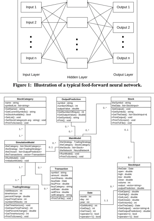
The other is from the machine learning community and consists of artificial intelligence and computer science techniques that allow for the creation of non-parametric models. These non-parametric models generalize data into models that can be used for classification, pattern recognition, and ultimately prediction. One of the foremost benefits of using non-parametric models is that they can accommodate nonlinear behavior without loss of information. These models work by mimicking the human brain and the interactions of the nervous system. A typical neural network contains an input layer, a hidden layer, and an output layer. The input layer receives the inputs for the model from various sources. The hidden layer acts as an intermediate step between the input and the output layers. Lastly, the output contains the different outputs of the model. There can be multiple nodes in each of these layers as is illustrated in Figure 1. The model works using each of the connections between the nodes. The connections have weights typically ranging from 0 to 1. When an input is received, a value is propagated through the hidden layer and on to the output layer. These values are then evaluated for the desired accuracy against expected values. Then, in an iterative fashion, the connections are adjusted during the learning process until the network produces the desired accuracy of results. A historic data set is used for both training and testing the efficacy of the neural network. The data are broken into a training set and a testing set. After running the training data, the network is tested against known data to assess the overall performance of the network.

DESIGN OF THE OBJECT-ORIENTED MODEL

The design for the Neural Network based simulation model is shown in Figure 2. The overall design is simplified by leaving out many of the basic get and set functions that accompany all of the classes. All data members are private by design and use public member functions to access the class data. Also, all classes use public constructors and most of the classes use overloaded constructors to accommodate all of the necessary instantiations. Similar to the set/get functions, these are not shown to simplify the illustration of the design. The description of the design first details the MainModel and its data members and then goes on to describe the simulation portion of the design. The MainModel class is central to the design. In fact, the MainModel class can be instantiated and run without creating a SimulationModel object. This allows the design to be extensible for future predictions as opposed to just running simulations based on previous data. The MainModel contains a TradingStrategy, a StockCategory, a list of the Stocks and a NeuralNetwork to process the data. It provides an OutputPrediction based on these data members and their respective settings. The OutputPrediction contains information that quantifies the correlation of the predictive value of the NeuralNetwork and the actual values of the previous data for the time frame specified in the TradingStrategy. Each Stock object contains data concerning the stocks of interest included in the StockCategory. The Stock objects contain information about the unique symbol of the stock and the list of data associated with that stock symbol. The data associated with each stock symbol is modeled as a StockInput object. This data (StockInput) includes the date of the data point, the opening price of the security, the high price for the day, the low price for the day, the closing price for the day and the volume of the security for that day. Also, output that is associated with each data point is stored in the StockInput object for use in other parts of the model. This simplifies the model and keeps the need for mapping this stored output information to a minimum. The SimulationModel can be instantiated to run simulations using previous data over any time period desired. A SimulationModel contains a list of StockCategories, a list of the TradingStrategies, a list of the chosen stock symbols based on the correlated output from the MainModel and a vector (array) of the transactions collected during the simulation run. The SimulationModel is designed to run any number of TradingStrategies over any number of StockCategories.

Thus, it is capable of storing any number of Transactions associated with the simulation. The design contains an entry point and for the simulation is assumed to be at the model run time. The exit point can be based on the price of the security either going above the percentChange times the entry price or going below the riskMeasure times the entry price. Since this is implemented within an Object-Orented framework, any amount of desired complexity can be added without affecting any other part of the design. A TradingStrategy contains basic information that a stock trader would be interested in utilizing but is completely disconnected from any category of stock. A TradingStrategy contains a measure for risk desired by the trader, a look-ahead time horizon for prediction purposes, a desired rise (or fall) in the price of the associated securities, the amount of previous days of data to use for prediction purposes and the number of Stocks to purchase for diversification. The TradingStrategy is flexible to involve both going short and going long within the strategy. A StockCategory contains information about the stocks of interest. Examples of StockCategories would be “S&P 500” and “FTSE 250”. Each StockCategory contains a name (such as the previously given examples) and a corresponding list of symbols within the category. Basic operations of a StockCategory allow the importing of the data associated with the category into the model as well as basic output.

METHODOLOGY

The methodology follows and extends much of the previous literature. First, a PNN is used based on the findings of both Gencay (1998) and Enke et. al. (2005). Leung et. al. (2000) state that multiple thresholds are useful for a PNN. They suggest this instead of using a basic cutoff point such as 0.5 for predictions. As such, the cutoff point for the PNN is an input variable which allows for testing different values. The hypothesis for this paper is that observed market data (volume, opening price, closing price, high price, low price and index level) contain enough pattern information to develop and employ a stock picking strategy that will outperform an index type investment. The hypothesis in this paper closely mirrors the work by Cichocki et. al. (2005) by capturing significant information from a reduced set of financial input data. A PNN is used to extrapolate that information for forecasting purposes.The data employed by the model are grouped into three categories, (1) trading strategy, (2) stock category, and (3) a listing of the actual stocks. The model first evaluates each stock individually and is then evaluated by the neural network during the training process. Next, the neural network predicts against known values and learns from its mistakes. The resulting process is a series of iterations which evaluates each of the stocks in the S&P 500 for all of the days in the time period. The time frame utilized for this study is March 2003 – August 2006.

The main parameters of the model are the trading strategy and the stock category. A trading strategy contains parameters for the risk tolerance (percent gain or loss allowed), the number of days of data to use for training the network, time horizon for the prediction, and the number of stocks to purchase. Trading strategies reflecting differing risk tolerances are easily accomplished. As such, a trading strategy that is risk averse could be developed to reduce the downside risk assumed. In the model tested for this paper, only the amount of positive change is specified. Another important aspect addressed by the PNN is the time horizon of the trading strategy. The model tested in this paper defines time horizon as the length of time into the future that the PNN is attempting to predict. The stock category defines the list of stocks to be considered by the PNN. In this study the S&P 500 is used as stock category. The symbols of all the companies in the index are used by the system to input the historical data for all the stocks. The model processes the data for each individual stock. The time required to simulate 16 weeks of data is approximately 60 minutes using a 3.0 GHz processor with 1 GB of RAM. During the process of evaluating each stock a correlation score is obtained that measures the relationship of the predictability of the PNN for each stock versus the actual results for the most recent data available. In its current state the model uses only positive relationships as information for predicting the profitability of stocks. Another possibility is to convert the model to use negative relationships that would indicate a decline in price.

To simplify the model, a constant investment of $1000 USD is used for each stock purchase. It is assumed that this amount will be used to purchase each stock and that the stock can be purchased in partial shares. Also, it is assumed that any profit is taken and any loss is returned at the end of each 16 week period. This allows for the constant investment previously mentioned. The model purchases up to a given number of stocks based on the trading strategy. The stocks are chosen from a list that has the highest correlations between the PNN’s predictions and known testing data. If the list has fewer entries in a given period than the desired number of stocks to purchase, the model purchases each of the stocks in the list. If the list has more entries, the model purchases the desired number of stocks based on the largest correlations.

The model’s selling rules are as follows. 1) The stock is sold if it reaches its low price, based on the risk tolerance of the trading strategy. 2) The stock is sold if it reaches its desired price at any time, based on the amount of change specified in the trading strategy. 3) The stock is sold at the closing price at the end of the period if the stock has surpassed neither the specified high nor the specified low prices. At the end of each period, the model steps back to the next period and simulates purchases in that period based on the next PNN generated choices. Taxes and transaction fees are assumed to be insignificant for this study. Stock data is downloaded from Yahoo.com and imported into the model. The model then removes the most recent period’s data for simulating the purchase and sale of individual stocks. The remaining data is used for training and testing the neural network. As is common when developing a neural network 75% of the data is used for training and the remaining 25% is used for testing the neural network. The choice of training and testing data results in some stocks being excluded due to lack of available data.

CONCLUSIONS

The contribution of this paper provides an Object-Oriented design for creating future implementations and extends the notion of using a PNN for predicting stock market winners. We presented a design and implementation of a PNN that can be used to test a wide variety of stock market trading strategies. It is discovered that the risk tolerance of the trading strategy gives its best performance in the 12-14% range. This is the amount of tolerance in the trading strategy for a loss on the purchase/sale of a given stock.

This parameter is tested below 12% and is found to be too sensitive. Many of the stocks chosen by the PNN often drop up to 10% of its purchased price before rebounding into a profitable scenario. Therefore, setting the risk tolerance below 12% caused the model to prematurely sell stocks at a loss that otherwise would have produced the desired profit. Also, it is discovered that the amount of desired change gives its best performance in the 16-19% range. This is near the peak level of performance of stocks before a market correction happens within the specified length of the prediction period. Results with the previously mentioned inputs produce a return of $4,780 over the horizon specified earlier (approximately 3 years and 5 months) for an initial investment of $5000. This approximately translates into an annualized return of 22.1%. This is calculated using the average return over each 16 week period. Since it was assumed that profit is taken or loss is replaced from/to the initial investment of $5000, a compounded rate-of-return is not calculated. This conservatively calculated return compares favorably with Ibbotson Associates reported returns for large cap stocks (15.397%), and long term corporate bond returns (4.802%) over the same time frame.

The inputs are tested to derive optimum profits. The most profitable prediction period is found to be 14-16 weeks. Running the model for less than 14 week predictions did not provide sufficient time for the stock price to grow. Running the model for more than the 16 week prediction period detracted from its ability to accurately predict short-term gains. The model had 1 out of 14 periods (16 weeks per period) where a 17.6% return was obtained. Overall, an average return of $341.43 was achieved for each of the periods tested. 3 out of 14 periods posted negative returns with a maximum loss of ($181.04) which translates to a 3.6% loss for that period. However, these losses are included in the overall profit figures. The results of this study are both significant and promising. Future improvements to this study include optimizing the parameters used for inputs, and testing different parameters. Data sets other than the S&P 500 should also be tested. Questions related to domestic versus international, small versus large companies, developed versus undeveloped stock markets, are all areas of possible future research.

REFERENCES

Bachelier, L. (1900) trans. James Boness. Theory of Speculation. in Cootner (1964), 17-78.

Balvers, R., Cosimano, T. & McDonald, B. (1990). Predicting Stock Returns in an Efficient Market. Journal of Finance, 55(4), 1177-1189.

Cichocki, A., Stansell, S., Leonowicz, Z., & Buck, J. (2005). Independent Variable Selection: Application of

Independent Component Analysis to Forecasting a Stock Index. Journal of Asset Management, 6(4), 248-259.

Dimson, E., & Mussavian, M. (1998). A Brief History of Market Efficiency. European Financial Management, 4(1), 91-193.

Enke, D., & Thawornwong, S. (2005). The Use of Data Mining and Neural Networks for Forecasting Stock Market Returns. Expert Systems with Applications, 29(4), 927-940.

Fama, E. (1965). The Behavior of Stock Market Prices. Jounal of Business, 38, 34-105.

Gençay, R. (1998). Optimization of Technical Trading Strategies and the Profitability in Security Markets. Economics Letters, 59(2), 249-254.

Hill, T., O’Connor, M., & Remus, W. (1996). Neural Network Models for Time Series Forecasts. Management Science, 42(7), 1082-1092.

Jasic, T. & Wood, D. (2004). The Profitability of Daily Stock Market Indices Trades Based on Neural Network Predictions: Case Study for the S&P 500, the DAX, the TOPIX, and the FTSE in the Period 1965-1999. Applied Financial Economics, 14, 285-297.

Lendasse, A., De Bodt, E., Wertz, V., & Verleysen, M. (2000). Non-linear Financial Time Series Forecasting – Application to the Bel 20 Stock Market Index. European Journal of Economic and Social Systems, 14(1), 81-91.

Leung, M., Daouk, H. & Chen, A. (2000). Forecasting Stock Indices: A Comparison of Classification and Level Estimation Models. International Journal of Forecasting, 16(2), 173-190.

Olson, D. & Mossman, C. (2003). Neural Network Forecasts of Canadian Stock Returns using Accounting Ratios. International Journal of Forecasting, 19(3), 453-467.

Samuelson, P. (1965). Proof That Properly Anticipated Prices Fluctuate Randomly. Industrial Management Review, 6, 41-49.

Schwert, W. (1990). Stock Returns and Real Activity: A Century of Evidence. Journal of Finance, 45, 1237-1257. Thawornwong, S., Enke, D. & Dagli, C. (2003). Neural Networks as a Decision Maker for Stock Trading: A

Technical Analysis Approach. International Journal of Smart Engineering System Design, 5(4), 313-325. Vellido, A., Lisboa, P. & Vaughan, J. (1999). Neural Networks in Business: A Survey of Application (1992-1998).

TABLES AND FIGURES Input 1 Input 2 Input n

.

.

.

.

.

_.

.

.

.

Hidden Layer Output Layer

Figure 1: Illustration of a typical feed-forward neural network.

+SetTimeHorizon() : void +GetInputTimeFrame() : int +GetPercentChange() : double +GetTimeHorizon() : int +PrintToScreen() : void -riskMeasure : int -timeHorizon : int -percentChange : double -inputTimeFrame : int -numberOfStocks : int TradingStrategy +GetNumberOfDays() : int +GetOutputValue() : double +GetSymbol() : string +Print() : void -symbol : string -numberOfDays : int -outputValue : double OutputPrediction +GetOpen() : double +GetHigh() : double +GetLow() : double +GetClose() : double +GetVolume() : int +GetTheDate() : Date +SetOutput() : vector<string>& +SetOutputPrediction() : double +operator>() : bool +operator==() : bool -theDate : Date -open : double -high : double -low : double -close : double -volume : int -output : vector<string> -outputPrediction : double StockInput +GetMonth() : int +GetDay() : int +GetYear() : int +operator>() : bool +operator==() : bool -month : int -day : int -year : int Date +GetName() : string +GetCurrentSymbolc() : string +IsStockAvailable() : bool +SetList() : void

+SetStockCategory(in arg : string) : void +PrintToScreen() : void -name : string -symbolList : list<string> StockCategory +RunModel() : void +InitializeModel() : void -theCategory : list<StockCategory> -theStrategy : list<TradingStrategy> -theChosen : list<OutputPrediction> -theTransactions : vector<Transaction> SimulationModel -SetOutput() : void +GetSymbol() : string +GetTheData() : list<StockInput>& +PrintOutput() : void +PrintToScreen() : void +PrintToFile() : void -theSymbol : string -theData : list<StockInput> Stock +RunModel() : void +PrintToScreen() : void -theStrategy : TradingStrategy -theCategory : StockCategory -theStocks : list<Stock> -theNetwork : NeuralNetwork MainModel 1..* 1..* 0..* 0..1 0..1 0..* 0..* 1..1 1..* 1..* +PrintToFile() : void -symbol : string -amount : double -numShares : double -buyDate : Date -buyPrice : double -buyCategory : string -sellDate : double -sellPrice : double -sellCategory : string Transaction 0..* 0..* 0..* 0..* 0..* 0..*