ARROW@TU Dublin
ARROW@TU Dublin
Dissertations School of Computing
2017
Application of Supervised Machine Learning to Predict the
Application of Supervised Machine Learning to Predict the
Mortality Risk in Elderly Using Biomarkers
Mortality Risk in Elderly Using Biomarkers
Priyanka SonkarTechnological University Dublin
Follow this and additional works at: https://arrow.tudublin.ie/scschcomdis
Part of the Computer Engineering Commons
Recommended Citation Recommended Citation
Sonkar, P. (2017) Application of supervised machine learning to predict the mortality risk in elderly using biomarkers. Masters dissertation, DIT, 2017.
This Dissertation is brought to you for free and open access by the School of Computing at ARROW@TU Dublin. It has been accepted for inclusion in Dissertations by an authorized administrator of ARROW@TU Dublin. For more information, please contact
[email protected], [email protected], [email protected].
This work is licensed under a Creative Commons Attribution-Noncommercial-Share Alike 3.0 License
learning to predict the mortality
risk in elderly using biomarkers
Priyanka Sonkar
A dissertation submitted in partial fulfillment of the requirements of
Dublin Institute of Technology for the degree of
M.Sc. in Computing (Data Analytics)
I certify that this dissertation which I now submit for examination for the award of MSc. in Computing (Data Analytics), is entirely my own work and has not been taken from the work of others save and to the extent that such work has been cited and acknowledged within the text of my work.
This dissertation was prepared according to the regulations for postgraduate study of the Dublin Institute of Technology and has not been submitted in whole or part for an award in any other Institute or University.
The work reported on in this dissertation conforms to the principles and requirements of the Institutes guidelines for ethics in research.
Signed:
The idea of long-term survival amongst older individuals has been a major medical and social concern. A wide range of biomarkers have been identified to prospectively predict disability, morbidity, and mortality outcomes in older adult populations. The machine learning techniques applied with clinically relevant biomarkers provide new ways of understanding diseases and solutions to tackle challenges to the health of the aging population.
This paper describes two supervised machine learning techniques, Logistic Regres-sion (LR) and Support Vector Machine (SVM) which are used in the prediction of the mortality in elderly people. LR is one of the traditionally used predictive modeling methods in clinical research where the probability of occurrence of two classes is a dichotomous criterion whereas, SVM is an emerging classification supervised learning technique based on building models using maximum-margin hyperplane. An attempt has been made to measure the classifier accuracy of each model and the performance of both the models is compared on a set of biomarker features of old patients. The experimental result shows that the SVM model outperformed the LR model in the prediction of survivorship among old individuals with statistically significant results (p<0.01).
Keywords: Mortality prediction, Biomarkers, Supervised Machine Learning, Lo-gistic Regression, Support Vector Machine
I would like to express my sincere gratitude towards my supervisor Dr. Luca Longo for his expert advice, constructive suggestions and enthusiastic encouragement and recommendations during the course of this research project.
I would also like to acknowledge Dublin Institute of Technology academic staff (DIT) especially my professors at School of Computing for their knowledge, help, guidance and kindness.
I would like to say thanks to my fatherJ.L. Sonkar, my motherRama Devi, my mother-in-law Promila Kher and my sisters Archana & Alka for their love, care, support and encouragement during my thesis.
Finally, I wish to say special thanks to my loving husband Vamshi Kher, who always believed in me and encouraged me to pursue masters in my area of interest. Your support and motivation gave me the strength to enhance my abilities and strive for academic and professional success.
Declaration I
Abstract II
Acknowledgments III
Contents IV
List of Figures VII
List of Tables IX List of Acronyms X 1 Introduction 1 1.1 Background . . . 1 1.2 Research project . . . 3 1.3 Research objectives . . . 3 1.4 Research methodologies . . . 4
1.5 Scope and limitations . . . 4
1.6 Document outline . . . 5
2 Review of existing literature 7 2.1 Mortality risk prediction . . . 8
2.1.1 Mortality . . . 8
2.1.5 Features to predict mortality . . . 11
2.2 Bio-markers . . . 12
2.2.1 Theory . . . 12
2.2.2 Biomarkers application . . . 13
2.2.3 Biomarkers based techniques . . . 15
2.3 Machine learning . . . 16
2.3.1 Unsupervised learning . . . 17
2.3.2 Supervised learning . . . 19
2.4 Application of machine learning in mortality prediction using biomarkers 21 2.5 Summary of literature, limitations and gaps . . . 23
3 Experiment design and methodology 25 3.1 Business understanding . . . 27
3.2 Data Understanding . . . 27
3.3 Data preparation . . . 29
3.3.1 SMOTE Algorithm: Balanced dataset . . . 29
3.3.2 Normalization and Standardization: Z-score . . . 31
3.3.3 One-Hot encoding: Categorical variables . . . 32
3.3.4 Random Forest Classifier: Feature importance . . . 32
3.4 Modeling . . . 33
3.5 Evaluation . . . 35
3.6 Strength and limitations . . . 38
3.7 Summary of design . . . 39
4 Implementation and results 40 4.1 Business Understanding . . . 40
4.2 Data understanding . . . 41
4.3 Data preparation . . . 46
4.4 Modelling . . . 48
4.4.1 Logistic regression: Balanced Target values . . . 49
4.4.2 Support vector machine: Balanced Target values . . . 50
4.4.3 Logistic regression: Imbalanced Target values . . . 52
4.4.4 Support vector machine: Imbalanced Target values . . . 53
4.5 Evaluation . . . 55
4.6 Summary of implementation . . . 56
5 Discussion and findings 57 5.1 Discussion . . . 57
5.1.1 Comparison of average accuracies of imbalanced and balanced target data . . . 58
5.1.2 Comparison of classifiers performance . . . 59
5.1.3 Statistical significance and hypothesis evaluation . . . 60
5.2 Strength and limitations of results . . . 61
5.3 Summary of analysis . . . 63
6 Conclusion 64 6.1 Research Overview . . . 64
6.2 Problem Definition . . . 65
6.3 Contributions and impact . . . 65
6.4 Future Work & recommendations . . . 66
References 68
A Mortality risk prediction code: Balanced dataset 74
1.1 Document Outline . . . 5
2.1 Literature review layout . . . 7
2.2 Age trajectory of mortality . . . 9
2.3 Validation of biomarkers . . . 13
2.4 Causal pathway from initiation to occurrence of disease . . . 14
2.5 Causal pathway from initiation to occurrence of disease . . . 16
2.6 K-means clustering for heart disease patients . . . 18
2.7 Accuracy v/s Precision . . . 19
2.8 Schematic representation of the optimum hyperplane by a SVM . . . . 20
3.1 CRISP-DM model . . . 26
3.2 High level design of the research experiment . . . 26
3.3 Sampling for Imbalanced data . . . 30
3.4 SMOTE algorithm KNN approach . . . 31
3.5 Standard normal distribution (Bell curve) . . . 32
3.6 Support Vector Machine . . . 34
3.7 Support Vector Machine kernels . . . 34
3.8 Stratified 5-fold cross validation technique . . . 35
3.9 ROC-AUC curve . . . 37
4.1 Statistical Analysis of data . . . 41
4.2 Distribution plot of numeric features with target . . . 42
4.6 Positive-Negative correlation with Target . . . 46
4.7 ROC curve: Logistic Regression . . . 49
4.8 ROC curve: Support Vector Machine - Linear . . . 51
4.9 ROC curve: Support Vector Machine - Radial . . . 51
4.10 ROC curve: Support Vector Machine - Polynomial . . . 52
4.11 ROC curve: Logistic Regression . . . 53
4.12 ROC curve: Support Vector Machine - Linear . . . 54
4.13 ROC curve: Support Vector Machine - Radial . . . 54
4.14 ROC curve: Support Vector Machine - Polynomial . . . 55
5.1 Model comparison using box-whisker plot: Unbalanced dataset . . . 58
3.1 Biomarkers information . . . 28
3.2 Confusion Matrix . . . 38
4.1 Missing Value Analysis . . . 42
4.2 SMOTE oversampling . . . 47
4.3 One-hot Encoding . . . 48
4.4 SVM kernels and tuning parameters . . . 50
4.5 SVM kernels and tuning parameters . . . 53
5.1 AUROC on imbalanced and balanced target (mortality risk) . . . 59
AUC Area Under the Curve
CRISP-DM Cross Industry Standard Process for Data Mining
CV Cross Validation
EMR Electronic Medical Records
FDA Food and Drug Administration
FN False Negative
FP False Positive
FPR False Positive Rate
GRSH General Self-Rated Health
HBV Hepatitis B Virus
IADL Instrumental Activities of Daily Living
ICU Intensive Care Unit
KNN K Nearest Neighbour
LOO Leave One Out
LR Logistic Regression
MSIA Mass Spectrometric Immunoassay
RBF Radial Basis Function
ROC Receiver Operating Characteristic
ROM Risk of Mortality
TN True Negative
TP True Positive
TPR True Positive Rate
Introduction
1.1
Background
In high-income countries, much of the health care spending are devoted to diseases where breakthroughs in diagnosis and treatment are elusive. Chronic diseases such as cardiovascular diseases, cancer, diabetes and chronic respiratory problems are serious challenges to the health of aging populations and health care budgets. The survey conducted by World Health Organisation in 2005 1, estimated that 60% of the global
mortality is due to chronic disease out of which 80% of this mortality occurred in low and middle-income countries (Tunstall-Pedoe, 2006).
Health challenges associated with aging is a major medical and social concern. Risk prediction functions have been used to generate risk scores for age-related macular degeneration, cardiovascular disease, Alzheimer, cancer, stroke or multi-organ failure leading to decreasing life expectancy (Rosero-Bixby & Dow, 2012)). Epidemiological observational studies have been conducted to quantify prevalence and risk factors for disease (Dipnall et al., 2016).
The biomarkers have been in use for centuries and play a crucial role in improving understanding of disease mechanisms and response of patient towards a particular therapy. Biomarkers are the genes or measurable indicators of a biological state used to diagnose disease state, stage of illness, risk, or treatment response (Dipnall et al.,
2016). The clinical use of biomarkers in drug development and medical diagnosis has recently accelerated the improvement in global health equity.
Although, biomarkers provide a powerful and dynamic approach in clinical stud-ies to understanding the spectrum of chronic disease or future death, it is necessary to identify potential biomarkers out of thousands of biomarkers of a patient. Diag-nostic tests are required for the translation of a biomarker into a clinically relevant biomarker, which includes generation and analysis of significant amount of data and knowledge. The generation of information is often logistically difficult, expensive and time-consuming. To overcome the hurdles associated with the generation of large amount of necessary data for the development of biomarkers, analysis techniques have been introduced.
The application of data mining techniques incorporating machine learning algo-rithms are rising across many disciplines over last two decades (Dipnall et al., 2016). In recent years, data mining techniques are used in the field of health care to analyze the massive amount of data to improve understanding of the disease and provide in-formation on the presence of disease or susceptibility to disease, in an individual, or monitor patient response to therapeutic interventions. Statistical classification tech-niques and Supervised Machine Learning algorithms such as Support Vector Machine, Neural Networks, Logistic Regression and Decision trees are commonly used to build predictive models for medical diagnosis (Maroco et al., 2011).
Traditionally, these predictive models had been implemented with organ-specific functional indicators (Rosero-Bixby & Dow, 2012) such as handgrip strength, walking speed, pulmonary peak flow which are associated with the mortality risk in a patient. The recognition of features that serve as early indicators in aging prediction is required to predict long-term survival in elderly (Pritom, Munshi, Sabab, & Shihab, 2016). To increase the prediction accuracy of the models, new variables such as biomarkers of the patient are used to build the models. Biomarkers applied with machine learning have the potential to transform the current health care model, from a reactive approach to one which is more proactive.
1.2
Research project
The aim of the project is to compare the performance of two supervised machine learn-ing techniques, Logistic Regression and Support Vector Machine for the classification of a group of elderly patients having mortality risk or not. The sample data set con-tains information about the biomarkers of the patient which is collected during the time span of three years by a doctor while monitoring her patients. The biomarkers of the patient are the independent feature variables which will be used to predict the target variable i.e. risk of mortality. Mortality risk predictive models will be built and later the comparison will be done based on the performance of the classifiers that have been trained on the same set of biomarkers data. Average accuracy of the classifiers will be used for evaluating the classifiers empirically. The research question answered from this project can be stated as:
“Can accuracy of models build with Support Vector Machine (SVM) for the predic-tion of mortality risk in elderly using biomarkers of the patients outperforms models build with Logistic Regression (LR) ?”
The results of the study would act as a proof of concept for the use of Support Vector Machine algorithms upon regression algorithms in the medical diagnosis.
1.3
Research objectives
The research objective of the project is to determine whether predictive models build with Support Vector Machine can yield greater classification accuracy than Logistic Regression model. In order to achieve the goal of the study, few experiments are performed as mentioned below:
• Explore the existing knowledge base on the application of machine learning in mortality risk prediction using biomarkers and perform a comprehensive analysis. • Select a sample of data set having information about the biomarkers of the
patients.
• Build mortality risk predictive models implementing Logistic Regression and Support Vector Machine algorithms.
• Compare models and select best prediction model evaluated based on the average classification accuracy in predicting the mortality risk.
1.4
Research methodologies
The study is focused on the comparison of two well-known machine learning algorithms in predicting survivorship among older individuals and hence comes under secondary research. The experiment will be performed on the existing dataset and no new data is collected for this study. As part of the Secondary research, literature related to similar research conducted on supervised machine learning techniques, mortality risk prediction, feature engineering for variable selection and biomarkers are studied to complete a comprehensive literature review.
The research methodologies used are Quantitative (Epidemiological) and empirical research. The experiment will be conducted to produce concrete results which will be further taken into consideration to address the hypothesis. The performance of the classifiers will be evaluated by comparing the average classification accuracy of each classifier. On the basis of the result, we will conclude which model turned out to be a better predictor and hence Inductive.
1.5
Scope and limitations
The study will focus on the prediction of the mortality risk by implementing machine learning techniques on the biomarkers of the patients. The dataset used for the ex-periment contains 37 biomarkers to study the impact of potential biomarkers on the chances of survival of an individual. Two supervised machine learning techniques, Lo-gistic Regression and Support Vector Machine will be used to build the models using biomarkers as independent features to predict the mortality risk (Verplancke et al., 2008). The models will be trained and then compared to discuss how they vary in
both their prediction performance and accuracy.
A limitation of our study is the relatively small sample size, only 93 records of patients are available for carrying out the experiment. Also, few of the predictor feature variables are not normalized. This can have a knock-on effect on the learning capability of the model as this may induce biasing in the results hence needed to be handled.
Furthermore, trends in the dependent variable (mortality risk) is again biased. There are approximately 20% of the records containing information with mortality risk as true, whereas 80% of the records have mortality risk as false. Data upscaling technique, SMOTE sampling will be used for data preprocessing while performing the experiment to get rid of small-sized biased data. Also, the research study will target only the elderly population and since mortality varies largely between age groups, our results cannot be automatically extrapolated to younger populations.
1.6
Document outline
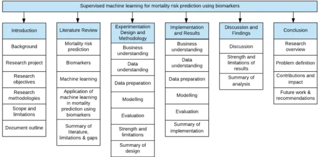
The layout of the report will be outlined as shown in figure 1.1, with six chapters in total, each divided into sections:
• Chapter 2 (Literature review) gives an overview of the current state-of-the-art relating to mortality prediction, biomarkers and supervised machine learning, primarily Logistic Regression and Support Vector Machine. A systematic litera-ture review has been conducted to gain an insight into the related work done in the prediction of the mortality risk in old age persons using supervised machine learning algorithms. The gaps in the existing research will be highlighted to propose the research question for this project.
• Chapter 3 (Experimentation design and methodology) will elaborate the design of the experiment having an explanation of each experiment to be performed and the motivation behind each step. A complete understanding of the data to be used will be outlined. Various techniques proposed to be implemented as part of the research will be listed and described in this chapter.
• Chapter 4 (Implementation and results) details the practical implementation of the experiments and describes the results obtained at each step.
• Chapter 5 (Discussion on findings) will provide the detailed analysis of the exper-imental results and based on the results, a decision will be made to either accept or reject the hypothesis. Lastly, this chapter will also elaborate the strength and weakness of the research.
• Chapter 6 (Conclusion) will summarize the findings of the research undertaken during the dissertation including problem definition, critical analysis of the de-sign, experiments conducted, evaluation of the results and scope for the further research.
Review of existing literature
This chapter provides a detailed review of the relevant literature to gain an insight into the related work done in the prediction of mortality risk in elderly using supervised machine learning and biomarkers. The review is broadly classified into three sections: mortality prediction, biomarkers and machine learning as shown in figure 2.1.
The state-of-art of the mortality risk prediction is presented in section 2.1 including the general theory about mortality, importance to predict mortality, various mortality risk prediction techniques and the features used to predict the mortality risk. The next section 2.2 provides details about biomarkers, explaining what are biomarkers, the application of biomarkers the and mortality risk prediction techniques based on biomarkers. The information and application of machine learning techniques in mor-tality risk prediction is given in section 2.3 which is further divided into unsupervised and supervised algorithms.
Last section 2.4 is the reflection of analysis of existing research around mortality risk prediction using machine learning algorithms with biomarkers. This analysis will help in finding the limitations and gaps in the existing research and motivation for the proposed research question.
2.1
Mortality risk prediction
2.1.1
Mortality
The risk of mortality (ROM) estimates the likelihood of death of a patient and provides a medical classification of patient mortality. Human mortality and the physiological processes of aging are fundamentally linked together and used in the process used to determine biological aging in human populations. The linkage between age and mortality is termed as the age dependence of mortality and is represented by Gompertz function (Manton, 1999).
The increased scientific knowledge has increased the average length of life or life expectancy in the developed or developing countries leading to weakening of this link-age (Manton, 1999). Figure 2.2 shows the link-age and mortality relation. The quadratic function is plotted for four ages (50, 59, 68 and 95 years) to analyze the impact of age on risk factor. Below figure 2.2 illustrates that the risk factor-age interaction is weak at age 50 and is maximum at age 95, infers that as age increases, mortality risk factor also increases.
Figure 2.2: Age trajectory of mortality (Manton, 1999)
2.1.2
Importance of mortality prediction
Several studies have been conducted to assess the general health of a person based on the survey rating provided by individuals as a response to the question how would you rate your health? excellent, very good, good, fair or poor. The score is useful in finding a rough estimate of the individuals who are not in a healthy condition and are seeking for medical assistance. As, per the experiment performed by DeSalvo, Bloser, Reynolds, He & Muntner in 2006, it is found that there is a statistically significant relationship between general self-rated health (GSRH) and high risk of mortality. Individual with poor GSRH had a 2-fold higher mortality risk as compared to the person with self-rated health as excellent (DeSalvo, Bloser, Reynolds, He, &
Muntner, 2006).
Health planners and policy makers are trying to find out a feasible method to identify the most vulnerable person with highest health requirements. GSRH can be used to improve the health care given to a patient through the identification of groups who are more susceptible to mortality risk. The collection of such data may help in offering a beneficial tool in health and care planning sector.
2.1.3
Mortality in elderly
The recognition of factors that contribute to healthy aging helps in the prediction of long-term survivorship among older individuals. A study is conducted by (Swindell et al., 2010) to identify predictors of long-term survival in older women. Individuals exhibiting healthy aging patterns maintain a high quality of life with very few daily living impairments whereas an unhealthy aging trajectory is associated with dimin-ished quality of life and increased mortality rate. The efficiency and quality of care can be improved by identifying at-risk individuals by predicting future health outcomes.
Prognostic information about the life expectancy of older people is important in clinical decision making and providing pro-active care to older people with limited life expectancy. In 2016, Houwelingen et al. conducted a study on 85-year-old inhabitants and collected samples over a time period of five years for mortality prediction. The collected sample of routine laboratory measurements was compared with gait speed and Instrumental Activities of Daily Living (IADL). It is concluded that the mortality risk predicted using laboratory tests are as accurate as models based on gait speed or IADL disability (van Houwelingen et al., 2013). In elderly aged >85 years, gait speed and IADL are predictors of survival where slow gait speed is associated with high risk of mortality. Also, the study supports that the poor ability in IADL was associated with a significantly higher 2-year mortality risk (Taekema, Gussekloo, Westendorp, de Craen, & Maier, 2012).
2.1.4
Mortality prediction techniques
Prediction of future health states can be significant in the medical domain as it can contribute to early detection of a disease, effective treatment and prevention. The health-related information of any individual is stored in Electronic Medical Records (EMRs) and can be used to generate accurate predictions for the occurrence of health issues in an individual and increasing risk of mortality. The two main approaches used for the prediction of mortality risk (Hoogendoorn, el Hassouni, Mok, Ghassemi, & Szolovits, 2016): (1) build a mortality predictive model based on the temporal features extracted from EMRs, and (2) defining a patient similarity matrix and predicting risk using the outcome of the similar patient.
2.1.5
Features to predict mortality
In order to extract the information contained in EMR data variety of approaches have been developed so as to fully exploit the wealth of information. The focus is on the extraction of features from EMRs and further to use these features for the generation of predictive models. As per Hoogendoorn, el Hassouni, Mok, Ghassemi & Szolovits these features can be implemented in commonly used classification approaches such as logistic regression or on defining patient similarity using instance-based learning such as K-nearest neighbor (KNN) approach. To select the most promising features correlation coefficient is calculated to find out the most correlated attributes. An iterative process is used where features with the highest correlation with the target (mortality risk) are selected (Hoogendoorn et al., 2016). A number of studies have been conducted to study the features which are responsible for the high mortality risk in patients. Previous studies have shown that there is a causal relationship be-tween the social relationships and the mortality rate (Holt-Lunstad, Smith, & Layton, 2010). Bixby and Dow explored few other most powerful mortality predictors: hand-grip strength, pulmonary peak flow, walking speed, blood markers, blood pressure and cholesterol level (Rosero-Bixby & Dow, 2012).
2.2
Bio-markers
2.2.1
Theory
The National Institutes of Health Biomarkers Definitions Working Group in 1998 defined biomarker as “a characteristic that is objectively measured and evaluated as an indicator of normal biological processes, pathogenic processes, or pharmacological responses to a therapeutic intervention ”(Strimbu & Tavel, 2010). Biomarkers come under the umbrella of medical signs which stands for the indicators or symptoms which help in identifying the health of a patient. Biomarkers include almost everything, the complex laboratory tests such as tissues or blood cells to the simplest characteristics such as pulse rate or blood pressure. Biomarkers are also considered as surrogates for individual clinical end-points (Strimbu & Tavel, 2010), which implies that a biomarker is capable of accurately predicting the clinical outcome i.e. physical or mental traits of a person.
The evaluation of biomarkers is necessary to identify it as surrogate endpoints which is done based on its relevance and validity. The relevance of a biomarker refers to its ability to provide clinically relevant information to health-care providers or to the public whereas validity refers the effectiveness of a biomarker as a surrogate endpoint. As per the studies conducted by Strimbu and Travel, the U.S Food and Drug Administration (FDA) has approved the use of biomarkers as surrogate endpoints in the treatment development process.
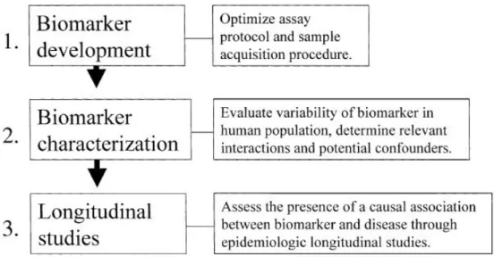
Groopman and Kensler developed a validation model to study development of hepatocellular carcinoma on exposure to aflatoxin B1 in humans (Bonassi, Neri, & Puntoni, 2001). This approach was designed for chemical-specific biomarkers, and is applicable to small scale only. Further, to provide a more general approach for the validation of biomarkers as early predictor of disease on humans, three steps process is designed as shown in figure 2.3.
Figure 2.3: Validation of biomarkers (Bonassi et al., 2001)
The first step is biomarker development which includes the evaluation of sensitiv-ity, sensibilsensitiv-ity, reliability and accuracy of the assay. The second step evaluates the variability of a biomarker in the human population. The last step is to assess the causal relationship between a disease and a biomarker. The validation process concen-trates on those biomarkers that are directly responsible in the prediction of a disease or mortality. The closer a biomarker to the causal pathway, more precisely it will help in the disease prediction (Bonassi et al., 2001).
2.2.2
Biomarkers application
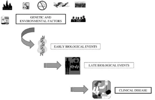
The major challenge of modern epidemiological research is to investigate the cause of a disease or death due to exposure to a potentially harmful substance (Bonassi et al., 2001). The knowledge of the harmful compound causing health issues can help in interrupting or eradicating a disease on time. In 1990, research has been conducted on biomarkers and molecules of individuals that lead to illness or disease are measured. The most promising feature of a biomarker is the ability to predict a disease and monitor public health. It plays a significant role in clinical research and medicines by providing insights into pathogenic mechanisms. The events that are on the direct
pathways from the initiation of the occurrence of a disease is shown in below figure 2.4. As suggested by Bonassi & Au, longitudinal studies are often required to study and evaluate the impact of biomarkers on clinical endpoints such as recurrence of cancer or survival (Bonassi & Au, 2002). As a substitute of long-term studies surrogate end points are created which are measured in short period of time.
Figure 2.4: Causal pathway from initiation to occurrence of disease (Bonassi & Au, 2002)
Biomarkers such as CD4 cell counts and HIV viral loads are proved beneficial for anti-AIDS treatments. Researchers have done an analysis to discover the root cause behind liver cancer and it is found that infection with hepatitis B virus (HBV) and exposure to a food-borne mutagen, aflatoxin (AFB1), are the major risk factors for liver cancer. Another example is to study the relationship between cigarette smoking and lung carcinogenesis. Almost 50% of the tumors having P53 gene and P53 mu-tation initiates lung cancer. Further clinical experiments showed that benzo[a]pyrene causes the mutation of P53 gene causing lung cancer (Bonassi & Au, 2002). Although biomarker helps in determining the potential treatments that are worth the efforts and resources, there is always a risk of false negative and false positives (Strimbu & Tavel, 2010). In terms of biomarkers, false negatives indicate the biological process
that led to improved clinical outcomes and is not captured by the biomarkers whereas, false positives indicate that biomarkers when used as surrogate outcomes do not pre-dict true clinical outcomes. Therefore, clinical endpoint analysis is important with biomarker analysis to avoid over reliance only on biomarkers.
2.2.3
Biomarkers based techniques
Over the years, epidemiological researchers have fused biomarkers with a number of techniques to recognize key biomarkers associated with a disease, leading cause of mor-tality among the patients. In 2011, Buddi, Taylor, Borges, & Nelson explored a lab-oratory based technique of Mass Spectrometric Immunoassay (MSIA) and discovered that MSIA is used to analyze potential biomarkers. MSIA is based on immunoassay technique which is used in biochemistry to detect an analyte in a solution. The first step of the process of MSIA is to attach antibodies to the MSIA tip. These antibodies are incubated with the antigen and antibody-antigen complex is washed repetitively to get rid of any non-specific antibody. Later, the bound antigen molecules are removed and antigens are extracted onto a mass spectrometer probe. This solution is dried and then molecular variants present in the sample are identified (Buddi, Taylor, Borges, & Nelson, 2011). The detailed process of MSIA is shown in figure 2.5. These clinically relevant biomarkers have a tendency to make distinctions with higher accuracy if used with machine learning techniques such as support vector machine classifiers.
Machine learning boosted regression algorithm and logistic regression can also be used to identify potential biomarkers (Song, Mitnitski, Cox, & Rockwood, 2004). Su-pervised machine learning techniques are now widely used to investigate the prediction of mortality using biomarkers along with non-linear techniques such as Support vec-tor machines, artificial neural networks etc. Supervised and unsupervised machine learning techniques are further elaborated in following section 2.3.
Figure 2.5: Causal pathway from initiation to occurrence of disease (Buddi et al., 2011)
2.3
Machine learning
Machine learning is a method of building analytical models by first performing data analysis to find hidden insights and using algorithms that iteratively learn from the historical data and helps in predicting unseen data. Machine learning offers advantages over statistical methods used for predictions i.e. easing the process of knowledge acquisition from a system or reducing the time consumption (Pietersma, Lacroix, Lefebvre, & Wade, 2003).
Day-to-day activities are comprised of machine learning techniques including, fraud detection, credit scoring, real time ads, pricing models, email spam filtering, text based sentimental analysis, medical diagnosis, pattern and image recognition, web search results and so on.
The biggest challenge in the field of health and sciences is to extract useful infor-mation from a large volume of data. Machine learning is now emerging as a solution
for the problem. Machine learning modelling methods such as supervised classifica-tion, clustering, probabilistic graphical methods for knowledge discovery, determinis-tic and stochasdeterminis-tic heurisdeterminis-tics for optimization are used in bioinformadeterminis-tics (Larranaga et al., 2006). According to the research conducted by Kononenko , the quality of the result depends on the selection of the classifier and concluded that combination of classifiers are more reliable in diagnostic systems problems instead of single classifier (Kononenko, 2001). Also, the classification performance is highly impacted by data preprocessing and tuning of algorithms (Pietersma et al., 2003).
The following sub-sections will give an overview of different classifiers which are broadly categorized as unsupervised and supervised machine learning techniques and their application in the prediction of the mortality risk among elderly.
2.3.1
Unsupervised learning
Unsupervised machine learning is used to draw inferences from unlabelled datasets. Cluster analysis is the most common unsupervised learning method to find grouping in data. The clusters are created based on the similarity measure such as Euclidean or probabilistic distance. The information in the resultant clusters are sorted in a way such that there are high intra-cluster similarity and low inter-cluster similarities (Gupta, Thakral, & Sharma, 2016).
Unsupervised algorithms are applied in data mining for pattern mining, sequence analysis and genetic clustering in bioinformatics, web mining, voice mining, medical imaging, and object recognition.
Nithya, Duraiswamy & Gomathy described few commonly used clustering tech-niques in their paper (2013). Hierarchical clustering has cluster nodes arranged in the form of a dendrogram containing child cluster, sibling clusters and parent node. Hierarchical clustering is further divided into agglomerative and divisive clustering. Inter-cluster similarity coefficients are calculated in agglomerative clustering and two similar clusters are merged into a new cluster. A divisive clustering has one cluster of all the data points at the beginning and further this cluster is split and recursive split-ting is applied until each pattern has its own singleton cluster (Nithya, Duraiswamy,
& Gomathy, 2013).
K-means clustering is another most favorable unsupervised clustering technique due to its elucidation simplicity, easy execution and flexibility to sparse information. According to Gupta, Thakral & Sharma normalization techniques may be used to improve the accuracy of k-means clustering, by clustering the remaining non-clustered points. K-means clustering is used to group persons into high and low risk of having heart disease by creating clusters of high blood pressure and cholesterol level as shown in figure 2.6.
Figure 2.6: K-means clustering for heart disease patients (Nithya et al., 2013)
The major drawback of k-means clustering is that it requires a number of clusters in advance and doesn’t fit to identify non-convex shaped clusters.
Furthermore, existing researches in genetics revealed that to understand the bio-logical processes, gene expression levels are measured at different development phases of different organisms, clinical conditions or body tissues. Traditional approaches to genomic research is based on the examination and collection of data from a single gene which is now extended to monitoring hundreds and thousands of genes under one experiment. Cluster analysis is used to analyze the tremendous amount of data obtained from micro-array studies (Tasoulis, Plagianakos, & Vrahatis, 2004). To im-prove the quality of clustering it is necessary to identify genes which have significant contribution.
Wang, Songtag & Wang in 2014 presented a disease progression modelling tech-nique based on unsupervised learning. The proposed approach is flexible to accom-modate new sources of data and further work can be done to modify existing model to learn a mixture of disease trajectories (Wang, Sontag, & Wang, 2014).
Similarly, supervised learning is another widely used machine learning technique in predictive modelling which is discussed in 2.3.2.
2.3.2
Supervised learning
Supervised classification technique is the most frequently carried out by Intelligent Systems and is applicable on the instances having labeled data. The supervised learn-ing is focused not just only on constructlearn-ing model by capturlearn-ing input features but also to provide robust prediction of the output i.e. accuracy and precision (Palmer & Chakravarty, 2014). Both accuracy and precision sound like the same thing but there is a major difference between both as accuracy refers to the lack of bias in predictions whereas precision refers to the lack of variance as shown in figure 2.7.
Figure 2.7: Accuracy v/s Precision (Palmer & Chakravarty, 2014)
The equation of a model that can be used to learn from existing data and to predict the outcome of new future data can be written as,
Y =f(X, θ) + (2.1) where, f(X, θ) represents a function that maps input X to input Y (Palmer & Chakravarty, 2014).
Binomial Logistic Regression (LR) is the traditional standard predictive modeling method used in clinical research and studies. LR models are basically used in building predictive models where the probability of occurrence of one of the two classes is a dichotomous criterion. Logit transformation gives linear combination of predictor and is given by below equation,
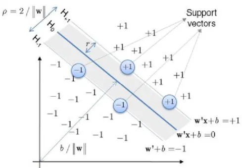
Figure 2.8: Schematic representation of the optimum hyperplane by a SVM (Maroco et al., 2011)
New artificial intelligence methods are emerging for classification purposes in med-ical diagnosis. Support Vector Machines (SVMs) are the newest supervised machine learning technique which revolves around the notion of a ‘margin’ i.e. a hyperplane as shown in figure 2.8, which separates the two data classes. Maroco et al. provided
insights that the generalization error can be reduced by maximizing the margin in order to create the largest possible distance between the separating hyperplane and the instances on either side of the hyperplane (Maroco et al., 2011).
Maroco et. al proposed a new hypothesis in the prediction of Dementia and cogni-tive impairment and concluded that an instance is classified into success group if the estimated probability is greater than 0.5 otherwise it is classified into failure group. The experimental results showed that newer statistical classification models such as neural networks, support vector machine and random forests results into improved accuracy, sensitivity and specificity (Maroco et al., 2011).
Similar researches have been done to compare the accuracy of the machine learning models in the prediction of mortality in critically ill patients. In 2008, Verplancke compared support vector machine and logistic regression models after trained these models using 252 patient records and validated it using rest 100 records. The area under the curve is used for validating the performance of the models and also statistical significance of the results is measured. The accuracy of both the classifiers comes out to be comparable but SVM has the possibility to improve patient care in near future by facilitating data modeling in the Intensive Care Unit (ICU) (Verplancke et al., 2008).
2.4
Application of machine learning in mortality
prediction using biomarkers
Gathering insights from the above sections, this section will provide information on the machine learning applications collaborated with biomarkers in mortality risk prediction in old individuals.
Machine learning algorithms are used to analyze medical datasets from the very beginning. The implementation of data mining techniques in medical field has im-mense potential for exploring hidden patterns in the data and utilize these patterns for clinical diagnosis. Medical diagnosis is the most complex task as it needs to be precise. This section will focus on the contribution of machine learning techniques in the area of research in medicine and epidemiology. Rose used prediction methods to
generate risk scores and risk prediction functions for timely detection of disease and to provide effective treatments to the patients based on the predicted risk of a disease or death (2013). Machine learning techniques are widely used to generate risk scores for heart disease, breast cancer, strokes and age-related physical performance. Prediction practices have initially relied on Parametric regression methods but now newer ma-chine learning methods such as random forests and neural networks are implemented for prediction. Researchers are working on the application of different techniques and investigating that which individual algorithm should be implemented on different datasets to derive better performance (Rose, 2013).
The increasing number of covariates including biological, clinical and genomic data, demands flexible algorithms that may capture potential predictor features. Therefore, dimensionality reduction or feature selection techniques has become an apparent need in the bioinformatics applications. Both feature selection and dimensionality reduction aim towards reducing the number of features and can be applied to both supervised and unsupervised learning. The most important objectives of feature selection identified by Saeys, Inza & Larranaga are (a) improve model performance by avoiding overfitting in the model, (b) to provide faster and cost-effective predictive model (c) to gain deeper insights of data generation and selection process (2007). However, the only overhead is that feature selection techniques increase the complexity of the model by introducing an additional layer in the modeling (Saeys, Inza, & Larra˜naga, 2007).
Hamid, Omar & Mabrouk in 2016 implemented correlation-based feature selection and chi-squared feature selection machine learning methods to find the most effective Single Nucleotide Polymorphisms (SNPs). These markers are useful in identifying geriatrics diseases (El Hamid, Omar, & Mabrouk, 2016) and achieved almost 76.70% accuracy using significant SNPs features. Similarly, Ding, Li & Wang proposed combi-nation of just-in-time learning (JITL) and extreme learning machine (ELM) in order to improve mortality prediction of ICU patients. JITL-ELM showed better perfor-mance in terms of area under the curve than neural network, logistic regression model and traditional score models (Ding, Li, & Wang, 2016).
2.5
Summary of literature, limitations and gaps
A review is presented in this chapter relating to the application of machine learning to identify the clinically relevant predictors for the prediction of geriatric chronic diseases leading to the mortality risk. Initially, literature related to the mortality risk are studied to gain knowledge about the risk of mortality in elderly, the importance of mortality predictions and the features for mortality prediction followed by biomarker’s literature focusing on biomarkers application and techniques. In machine learning section emphasis is given on two supervised machine learning techniques, Logistic Regression (LR) and Support Vector Machine (SVM) which are applied in the area of medical sciences.
Non-linear techniques such as support vector machine with polynomial kernels and radial basis functions (RBF) need to be investigated in future by researchers. These relationships are desirable to be discovered but a prior experiment is needed to interpret the importance of nonlinear techniques on a particular dataset (Song et al., 2004). Also, Delen, Walker & Kadam suggested that better promising methods such as support vector machines and rough sets can be used over decision trees, artificial neural networks and logistic regression in order to improve the prediction accuracy (Delen, Walker, & Kadam, 2005). In their further research, they proposed to implement a hybrid intelligent system. In a hybrid system, data mining results would be augmented with expert opinions and captured into an expert system. Liu emphasized on the comparison of different models to obtain better results (Liu, 2007).
According to the simulations performed by Liu, variable selection and survival function estimation of highly correlated features can prove beneficial for medical diag-nosis (Liu, 2007). Hamid, Omar and Mabrouk worked on the identification of genetic biomarkers associated with Alzheimer’s disease. Different gene selection methods to discover new biomarkers using machine learning algorithms can be further explored as Phase II of this work (El Hamid et al., 2016). Fuzzy rule extraction method is used by Pal in 2007 to find a small set of most important features to build the model out of thousand of available features. It is found that different set of algorithms identify
different sets of important features hence investigations should be undertaken to set a threshold for the modulator values (Pal, 2007). The identification of the most effective biomarkers and accuracy of classifier on the number of features is suggested by Buddi, Taylor, Borges & Nelson for future research (Buddi et al., 2011). Biomarkers such as hypertension, hypercholesterolemia and stress can be explored and used for prediction (Gruenewald, Seeman, Ryff, Karlamangla, & Singer, 2006), (Rosero-Bixby & Dow, 2012).
The gaps and limitations are addressed by proposed research question which is given as,
“Can accuracy of models build with Support Vector Machine (SVM) for the predic-tion of mortality risk in elderly using biomarkers of the patients outperforms models build with Logistic Regression (LR) ?”
Following sections will elaborate the design, methodology and experiments per-formed to answer the research question.
Experiment design and
methodology
This chapter will elaborate the plan and design of the experiments proposed to answer the research question. The standard approach of the CRISP-DM process (Chapman et al., 2000) will be implemented which is a structured data mining project planning methodology. The experiment will be carried out in five phases i.e. business under-standing, data underunder-standing, data preparation, modeling and evaluation. All the experimental steps will be performed in Python language using scikit-learn library. Scikit-learn (Scikit-learn.org, 2017) is an open machine learning library featuring var-ious classification, regression and clustering algorithms.
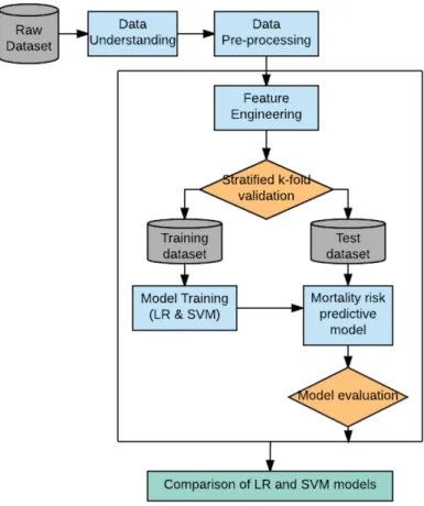
The main aim of the research is to build a mortality risk predictive model based on the historical data of biomarkers of elderly patients which has been collected over a time span of three years. The chapter is divided into sub-sections adhere to CRISP-DM framework as shown in figure 3.1. Subsequent subsections will provide detailed information of the experiment.
Figure 3.1: CRISP-DM model (Chapman et al., 2000)
The high-level experiment of the research is illustrated in below figure 3.2:
3.1
Business understanding
The key focus of the study is to compare two supervised machine learning algorithms for the prediction of mortality risk. In order to achieve the primary goal of the research two models will be trained on the data containing biomarker features of the patients. Later the performance of both the models will be evaluated using average classification accuracy of the models. The following hypothesis will be taken into consideration to address the research question:
“H0 The accuracy of the model built with Support Vector Machine outperforms Logistic Regression for prediction of the mortality in elderly using bio-markers of the patient, with p-value <0.01.”
3.2
Data Understanding
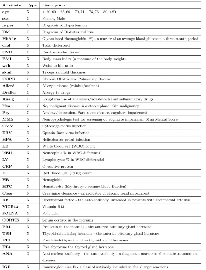
The dataset contains information about the mortality risk factors in community dwelling elderly which had been collected from a European hospital during a time span of three years. This dataset consists records of 93 patients and information about 37 different biomarker features of each individual as shown in table 3.1. The age-group of the patients are divided into six categories i.e. <60, 60-65, 66-70, 71-75, 76-80, >80.
The mortality risk of the patient is the dependent variable and may take values either ‘0’ or ‘1’. The predictor variables are both continuous and categorical in nature. Table 3.1 contains the summary of the dataset, where attributes are the biomarkers and type represents the data type of each variable i.e. ‘N’ for numeric values and ‘C’ for categorical values.
Data investigation will be performed using Python code and include following steps: 1. Statistical analysis: Basic statistics such as distribution, average, max, min, standard deviation, normalization, mode, the skewness of variables will be com-puted for analysis.
2. Missing value analysis: Count and percentage count of the missing values of target and predictor variables will be calculated.
Attribute Type Description
age N <60,60−65,66−70,71−75,76−80, >80
sex C Female, Male
hyper C Diagnosis of Hypertension DM C Diagnosis of Diabetes mellitus
HbA1c N Glycosilated Haemoglobin (%) - a marker of an average blood glucosein a three-month period chol N Total cholesterol
CVD C Cardiovascular disease
BMI N Body mass index (a measure of the body weight) w/h N Waist to hip ratio
skinf N Triceps skinfold thickness
COPD C Chronic Obstructive Pulmonary Disease Allerd C Allergic disease (rhinitis/asthma) Draller C Allergy to drugs
Analg C Long-term use of analgesics/nonsteroidal antiinflammatory drugs Neo C No, malignant disease in a stable phase, skin malignancy Psy C Anxiety/depression, Parkinsons disease, cognitive impairment
MMS N Neuropsychologic test for screening on cognitive impairment Mini Mental Score CMV N Cytomegalovirus infection
EBV N Epstein-Barr virus infection HPA N Helicobacter pylori infection LE N White blood cell (WBC) count NEU N Neutrophils % in WBC differential LY N Lymphocytes % in WBC differential CRP N C-reactive protein
E N Red Blood Cell (RBC) count
HB N Hemoglobin
HTC N Hematocrite (Erythrocyte volume blood fraction)
Clear N Creatinine clearance - an indicator of chronic renal impairment
RF N Rheumatoid factor - the auto-antibody, increased in patients with rheumatoid arthritis VITB12 N Vitamin B12
FOLNA N Folic acid
CORTIS N Serum cortisol in the morning
PRL N Prolactin in the morning - the anterior pituitary gland hormone TSH N Thyroid-stimulating hormone - the anterior pituitary gland hormone FT3 N Free triiodothyronine - the thyroid gland hormone
FT4 N Free thyroxine the thyroid gland hormone
ANA N Anti-nuclear antibody - the auto-antibody - a diagnostic marker in rheumatic autoimmune diseases
IGE N Immunoglobuline E - a class of antibody included in the allergic reactions
3. Outlier analysis: Outlier analysis will be performed to find out the values lying out of range eg. age group of patients.
4. Exploratory data analysis: Frequency distribution plots of numeric and categor-ical variables with respect to the target variable.
5. Heatmap correlation matrix: Heatmap matrix will be produced to analyze the correlation between the target variable (mortality risk) with the predictor vari-ables (biomarkers). Also, a separate plot will be generated to understand if the variables are positively or negatively correlated with the target variable.
The next section provides the detailed overview of the steps carried out for data preparation and feature engineering used for the research work.
3.3
Data preparation
The data preparation phase covers all the activities involved in the transformation and cleaning of the data to make it fit to use in the modeling phase (Learn, 2017). The missing values, noise and outliers present in the data identified during data under-standing phase will be removed in data pre-processing. The identified missing values will be imputed using the mean value of the variable.
3.3.1
SMOTE Algorithm: Balanced dataset
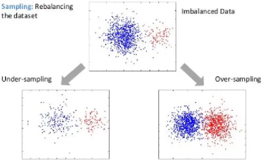
The main concern is that the data is highly imbalanced and small in size. There are approx. 20% records which have mortality risk as ‘1’ and rest 80% of records have mortality risk as ‘0’. If the experiment is proceeding further to modeling phase without balancing the data then the model will be trained with biasing and cost of mis-classifying minority class could be very high. Sampling techniques: under-sampling or over-sampling as shown in figure 3.3, should be implemented to get rid of imbalanced data set.
Figure 3.3: Sampling for Imbalanced data (Walimbe, 2017)
Since the data set is quite small in size, each instance is highly important and can’t risk to loosing any information. Hence, under-sampling technique is discarded and over-sampling technique will be used for the experiment.
Synthetic Minority Over sampling Technique (SMOTE) algorithm will be used for creating synthetic samples. SMOTE applies KNN approach where it selects K nearest neighbors, joins them and creates the synthetic samples in the space as shown in figure 3.4. The algorithm takes the feature vectors and its nearest neighbors and computes the distance between these vectors. The difference is multiplied by a random number between (0, 1) and it is added back to feature.
Figure 3.4: SMOTE algorithm KNN approach (Walimbe, 2017)
3.3.2
Normalization and Standardization: Z-score
Learning algorithms are known to provide reckless predictions on unscaled or unstan-dardized features. To ensure that all the feature values are on the same scale, nor-malization or standardization is a mandatory step to be carried out before proceeding to model building. Standardization is a preprocessing step to standardize values of features from different dynamic range into a specific range.
Standard score or commonly known as z-score converts scale of all the parameters having zero mean and unit variance and can be given as,
zi =
xi−x
S (3.1)
where, ¯
x is the mean of the sample
S is the standard deviation of the sample
A z-score can be placed on a normal distribution curve as shown in figure 3.5. Z-scores range from -3 standard deviations to +3 standard deviations.
Figure 3.5: Standard normal distribution (Bell curve)
3.3.3
One-Hot encoding: Categorical variables
The biomarker data set has 10 categorical variables out of 37 feature variables. In order to build LR and SVM model, categorical variables need to be converted into numeric variables as regression analysis and vector machine only work on numeric variables. To overcome this problem, dummy variables will be constructed out of categorical variables using pandas library in python.
3.3.4
Random Forest Classifier: Feature importance
Lastly, to find out the importance of each variable in predicting the mortality risk, Random Forest algorithm will be applied (Svetnik, Liaw, & Tong, 2004). Random Forest is an ensemble modeling technique which is based on iteratively removing low-ranking variables and assessing the learning performance by cross-validation.
A score will be generated for each variable which provides the importance of the variable in the model. Highest the score of the variable, highest the importance of that particular variable. Variables with the lowest score may be considered as least impor-tant and can be eliminated. Data pre-processing techniques help in the extraction of more useful information and build a model with higher accuracy and performance.
3.4
Modeling
The main aim of this study is to investigate the use of a Support Vector Machine (SVM) based classification model for determining the mortality risk by comparing it with Logistic Regression (LR) based classification model. Therefore, two supervised machine learning algorithms, Logistic Regression and Support Vector Machine will be implemented to build the models.
Logistic regression is the most commonly used prognostic modeling method whereas, support vector machine is relatively new classification method which has been devel-oped by Vapnik et al. in 1990s as a result of the collaboration between the statistical and the machine learning. The target variable is categorical with binary values (0,1), hence logistic regression is fit to use for the prediction of the mortality risk amongst other regression techniques. The LR method uses a weighted least squares algorithm, i.e. the prediction is based on the construction of a regression line as the best fit through the data points by minimizing a weighted sum of the squared distances to the fitted regression line (Verplancke et al., 2008).
Logistic regression is based on logistic function σ(t) which is defined as follows:
σ(t) = e
t
et+ 1 =
1
1 +e−t (3.2)
SVM is also a supervised machine learning technique similar to LR which is used for both regression and classification problems. SVM, in contrast, tries to model the input variables by finding a boundary for the classification of target variable which is called hyper-plane. The data points nearest to the hyper-plane are the support vectors and are considered as the critical elements of the data set because the removal of the points will lead to the alteration of the dividing hyper-plane. SVM can be used for both regression and classification purposes. If no separation is possible within a high number of input variables, the SVM algorithm finds a separation boundary for the classification as shown in figure 3.6. The separation boundary is generated by transforming the input variables by increasing the dimensionality of the variable space.
Figure 3.6: Support Vector Machine (Verplancke et al., 2008)
Three different SVM models will be built as part of the experiment which consists of SVM Linear kernel model, SVM radial kernel model and SVM polynomial kernel model each tuned with different values of tuning parameter ‘C’ and ‘γ’. SVM model uses a kernel function to separate classes which can’t be separated using line or plane. Therefore, a non-linear region is required by the classifier to separate such classes. This is also known as kernel trick, transformation of the data into higher dimensional feature space in order to separate it linearly as shown in figure 3.7.
3.5
Evaluation
This experiment uses two steps to evaluate the performance of the predictive models. Firstly, a Stratified K-fold cross validation technique will be used for the validation of the model. In stratified k-fold cross validation, the folds are selected in such a way that each class labels are equally distributed in each fold. The target variable is binary and hence the experiment comes under dichotomous classification, this means that each fold contains roughly the same proportions of the two types of class labels. The data set will be divided into k subsets where k =10, each time one of the k subsets will be used as the test set and the k-1 subsets will be used as a training set. In this way, every data point will be part of the test set exactly once and gets to be in training set k-1 times. The average results from the k folds will be taken and single estimation will be produced. The only disadvantage of using k-fold cross validation is that the algorithm takes time for training. k=10 is the standard value which is ideally used in the experiments. The training and test split in 5-fold cross validation is shown in below figure 3.8:
Figure 3.8: Stratified 5-fold cross validation technique (Slideshare.net, 2017)
in the prediction of mortality risk. Accuracy of the model will be computed in each fold and in the end there would be 10 accuracies per model. Accuracy of the model is given as,
Accuracy= T P +T N
T P +F P +F N +T N (3.3)
where,
TP (True Positive) i.e. positive instances that are classified as positive, FP (False Positive) i.e. negative instances that are classified as positive, FN (False Negative) i.e. positive instances that are classified as negative, TN (True Negative) i.e. negative instances that are classified as negative
The evaluation parameters such as, average classification accuracy, receiver opera-tion curve (ROC) (Verplancke et al., 2008) and area under the curve (AUC) (Wu, Roy, & Stewart, 2010) will be obtained. ROC-AUC plot of each model will be generated to visualize the mean accuracy of each model. ROC curve is based on two metrics, True Positive Rate (TPR) and False Positive Rate (FPR).
True positive rate (TPR), also known as sensitivity, hit rate or recall,is defined as
T P R= T P
T P +F N (3.4)
Intuitively this metric corresponds to the proportion of positive data points that are correctly considered as positive, with respect to all positive data points. In other words, the higher TPR, the fewer positive data points will be missed.
False positive rate (FPR) or fall-out is defined as
F P R= F P
F P +T N (3.5)
FPR can also be generated from specificity as
F P R= 1−Specif icity (3.6) where specificity is defined as
F P R= T N
This metric corresponds to the proportion of negative data points that are mistak-enly considered as positive, with respect to all negative data points. In other words, higher the FPR, the more negative data points will be missclassified.
Figure 3.9: ROC-AUC curve
In order to combine FPR and TPR into one single metric i.e. to generate AUC, two former metrics with different threshold is calculated and then plotted on a single graph with FPR values on x-axis and TPR values on the y-axis. The resulting curve is called AUROC as shown in figure 3.9.
A confusion matrix is another evaluation metric which is used to describe the per-formance of a classifier by calculating evaluation parameters and is shown in table 3.2. The values of true positive rate and false positive rate are generated using confusion matrix.
Actual Positive Actual Negative
Predicted Positive TP FP
Predicted Negative FN TN
Table 3.2: Confusion Matrix
The comparison of both the models will be helpful in finding out the performance difference between the models in terms of classification accuracy. The final step is to determine the statistical significance of each experiment and to accept or reject the stated hypothesis. ‘Wilcoxon Signed-Rank Test’ will be used to test the statistical significance with p-value set as 0.01.
3.6
Strength and limitations
This section outlines the strength and limitations of the research design. Firstly, two different families of models (Regression and SVM) are adopted to perform an experiment which is believed to be effective in order to gain insight of performance of distinct models on the mortality risk prediction. Regression is known to provide better interpretability and information about the significance of the predictive feature based on the coefficients assigned to each feature whereas, SVM has higher predictive power. Also, different SVM models with linear, radial and polynomial kernels will be trained on the data set with an optimal level of tuning.
The models will be trained using stratified 10-fold cross validation technique and should gives more accurate predictions. The model will be trained and evaluated 10 times and hence the average of all the accuracies obtained in 10 iterations will be taken to evaluate the classifier accuracy.
The major limitation of the study is the relatively small size of dataset, only 93 records of patients are available against 37 predictor variables. In general, for binary values there should be 2npossible cases for ’n’ features. Higher the number of predictor
features, higher the number of samples used to train the model. In real life, model can’t be trained for all possible number of combinations but it is good to use maximum
possibilities so that model can learn the exact behavior of target variable vs predictor variables.
Secondly, trends in the dataset are biased, records containing information with mortality risk as true are (1/4)thof the records with zero mortality risk. Synthetic data
samples are created using data upscaling technique. This might produce difference in the results obtained using real world sample data and synthetic data.
Lastly, extensive tuning of SVMs models is not proposed while training the model due to time constraints and insufficient computational powers.
3.7
Summary of design
This chapter is dedicated to providing the breakdown of the experiment to be carried out for the thesis. The strength and limitations of the experiments are also proposed in this chapter.
The chapter starts with a brief description of the dataset including the variable types and data source. One of the main concern are the issues present in the raw data. Hence, data pre-processing machine learning techniques are briefed which will be used for cleaning and normalizing the data to make it fit for modeling. These pre-processing techniques include SMOTE algorithm to balance dataset, Z-score for data standardization and One-hot encoding to generate dummy variables.
Further, four different models will be trained, LR, SVM with linear kernel, SVM with radial kernel and SVM with polynomial kernels. In the end, evaluation of all the models will be done and best model will be selected based on the average classification accuracy of each model.
The following chapter details the practical implementation of the proposed design and experiments.
Implementation and results
This chapter details the results of the experiments performed. The layout of the chap-ter is a mirror of the previous chapchap-ter ’Design and Implementation’ so that comparison can be made between the proposed design of each phase and the actual results obtained for that phase.
4.1
Business Understanding
The primary goal of this section as outlined in the previous chapter is reproduced here. This section will ensure that the targets are met according to the phases.
1. Exploratory analysis of input dataset.
2. Missing value and outlier analysis followed by data cleaning. 3. Impute missing values and generate dummy variables. 4. Train models on feature sets.
5. Score each model and analyze the results.
6. Compare the models in order to answer the research question. 7. Evaluate the statistical significance of the results.
4.2
Data understanding
The descriptive statistics of data is shown in Figure 4.1. The target variable is binary and has value either ’1’ i.e. mortality risk is true or ’0’ i.e. no mortality risk. The table provides information about the mean, standard deviation, maximum value, minimum value and distribution (quartile range) of each numeric variable.
Figure 4.1: Statistical Analysis of data
The Count column provides the information about the total number of records of each variable. Only three biomarkers, ’CRP’, ’Clear’ and ’TSH’ has missing value out of 37 variables and is given in table 4.1.
Variable Missing Count Missing Percent
Clear 1 0.010753
TSH 1 0.010753
CRP 1 0.010753
Table 4.1: Missing Value Analysis
Figure 4.2 and 4.3 shows the distribution of the numeric features with respect to the target variable. BMI, CMV, CORTIS, Chol, Clear, E, FOLNA, FT3, FT4, HB, HTC, LE, LY, MMS, NEU, VITB12, age, skinf and w h are normally distributed with the mortality risk. Biomarkers such as ANA, CRP, HPA, HbA1c, IGE, TSH are positively skewed whereas, EBV is negatively skewed.
Figure 4.3: Distribution plot of numeric features with target
The frequency plot of categorical variables; sex, hypert, DM, CVD, COPB, aller d, d aller, analg, neo, Psy is plotted as shown in figure 4.4. The ‘Target’ variable is highly biased as per the information provided by the bar graph. Only 20% of the values are ’1’ and rest of the records have ’0’ values. The number of patients having high mortality risk is almost (1/4)th of the number of patients without any mortality risk. The balancing of the target feature will be taken care of in Data Preparation section.
All the categorical variables are binary and have ’Yes’ or ’No’ values except DM which has 3 distinct values as shown in figure 4.4.