A Machine Learning System for Automated Whole-Brain Seizure
Detection
ABSTRACT
Epilepsy is a chronic neurological condition that affects approximately 70 million people worldwide. Characterised by sudden bursts of excess electricity in the brain, manifesting as seizures, epilepsy is still not well understood when compared with other neurological disorders. Seizures often happen unexpectedly and attempting to predict them has been a research topic for the last 30 years. Electroencephalograms have been integral to these studies, as the recordings that they produce can capture the brain’s electrical signals. The diagnosis of epilepsy is usually made by a neurologist, but can be difficult to make in the early stages. Supporting para-clinical evidence obtained from magnetic resonance imaging and electroencephalography may enable clinicians to make a diagnosis of epilepsy and instigate treatment earlier. However, electroencephalogram capture and interpretation is time consuming and can be expensive due to the need for trained specialists to perform the interpretation. Automated detection of correlates of seizure activity generalised across different regions of the brain and across multiple subjects may be a solution. This paper explores this idea further and presents a supervised machine learning approach that classifies seizure and non-seizure records using an open dataset containing 342 records (171 seizures and 171 non-seizures). Our approach posits a new method for generalising seizure detection across different subjects without prior knowledge about the focal point of seizures. Our results show an improvement on existing studies with 88% for sensitivity, 88% for specificity and 93% for the area under the curve, with a 12% global error, using the k-NN classifier. Keywords: Seizure, non-seizure, machine learning, classification, electroencephalogram, oversampling
1. INTRODUCTION
Epilepsy is a chronic condition of the brain, and causes repeated seizures, commonly referred to as fits. Epilepsy is said to affect one in every 103 people in the UK (500,000 approximately) according to epilepsy research UK1, and 70 million people worldwide [1]. The risk of developing epilepsy is greatest at the extremes of life with incidences more common in the elderly than the young [2] and is the cause of premature mortality for those suffering with the condition [1].
Seizures can be focal (partial) and exist in one part of the brain only, or they can be general and affect both halves of the brain. In a focal seizure, the excess electrical activity is confined to the occipital lobes, parietal lobes, frontal lobes, or temporal lobes. During a focal seizure, the person may be conscious and unaware that a seizure is taking place, or they may have
uncontrollable movements or unusual feelings and sensations. During a general seizure, consciousness is normally lost and muscles may stiffen and jerk2. A diagnosis of epilepsy is made if a patient has had two or more unprovoked seizures3, and with the help of an electroencephalogram (EEG), which measures the electrical activity in the brain. EEG recordings are commonly visualised as charts of electrical energy plotted against time, which medical experts study, sometimes for days, in an attempt to detect the patterns produced by seizures [3].
The majority of previous works on seizure detection and prediction have focused on patient-specific predictors, were a classifier is trained on one person and tested on the same person [4]–[11]. However, in this paper, the emphasis is on using EEG classification to generalise detection across all regions of the brain using multiple subject records, without prior knowledge of which region of the brain the seizure occurred.
A whole-brain seizure detection approach supports para-clinical evidence obtained from magnetic resonance imaging and EEG to make a diagnosis of epilepsy and instigate treatment earlier. More importantly, it mitigates the difficulties associated with the capture and interpretation of electroencephalogram by neurologists, which reduces the costs associated with the training of specialists to perform the interpretation. In this paper, a robust data processing methodology is adopted and several classifiers are trained and evaluated, using 342 EEG segments (171 seizures and 171 non-seizures) extracted from the EEG records of 24 patients suffering with epilepsy.
The structure, of the remainder, of this paper is as follows. Section 2 describes the underlying principles of EEG and the type of features extracted from EEG signals. Section 3 discusses machine learning and its use in seizure and non-seizure classification, while section 4 describes the evaluation. The results are discussed in Section 5 before the paper is concluded in Section 6.
2. SEIZURE DETECTION AND CLASSIFICATION
Gotman is one of the pioneers of seizure detection whose research in the area dates back to 1979. In [12], he proposed a system for automatic recognition of inter-ictal epileptic activity in prolonged EEG recordings using a spike and sharp wave recognition method. Extensions to this work are presented in [13]–[16], while recent works have focussed on the use of functional magnetic resonance imaging (fMRI) and the correlation between cerebral hemodynamic changes and epileptic seizure events visible in EEG [17]. More recently, he has looked at automatic seizure detection in sEEG using high frequency activities in the wavelet domain [7].
In other studies, classification has featured widely in EEG research. The most common classifier used to distinguish between seizure and non-seizure events has been the support vector machine (SVM). Using the CHB-MIT database and a patient-specific prediction methodology, the study in [18] used a SVM classifier on EEG recordings from 24 subjects. The results show that a classification accuracy of 96% for sensitivity was produced, with a false-positive rate of 0.08 per hour. In a similar study five patient records from the CHB-MIT
2 http://www.epilepsy.org.uk 3 http://www.who.int
dataset containing a total of 65 seizures were evaluated using a linear discriminant analysis classifier [19]. The results show that 83.6% was achieved for sensitivity, 100% for specificity, with an overall accuracy of 91.8%. Nasehi et al. [20] used the same CHB-MIT dataset with a Particle Swarm Optimisation Neural Network (PSONN) which produced 98% for sensitivity and a false-positive rate of 0.125 per hour. The main difference with all of these studies, compared with the approach taken in this paper, is they are patient specific and do not generalise across a wider population.
In [21], 100 seizure segments and 100 non-seizure segments were used to train an SVM classifier. The results show that 100% was obtained for sensitivity, specificity and overall accuracy. Meanwhile, Nicoletta et al. [22] carried out a similar study using the BONN dataset [21] and SVM classifier, with 94.38% for sensitivity, 93.23% for specificity and an overall accuracy of 86.1%. In a similar study, Ubeyli [23], who also used the BONN dataset [21] and SVM classifier, produced 99.25% for sensitivity, 100% for specificity and 99.3% for overall accuracy. Extending this study, Ubeyli compared seven different classifiers. The SVM was the best-performing classifier with similar results produced to those in the original study [24]. The worst performing classifier was the multilayer perceptron neural network, which achieved 90.48% for sensitivity, 97.45% for specificity, and 90.48% for overall accuracy. Acharya et al. focused on using entropies for EEG seizure detection and seven different classifiers [25]. The best-performing classifier was the Fuzzy Sugeno classifier, which achieved 99.4% for sensitivity, 100% for specificity, and 98.1% for overall accuracy. The worst performing classifier was the Naïve Bayes Classifier, which achieved 94.4% for sensitivity, 97.8% for specificity, and 88.1% for accuracy. In [26], the decision tree classifier was used and achieved an average sensitivity of 99.24%, a specificity of 98.76%, and accuracy of 99.02%.
Using the FRE4 datasetYuan et al. presented a patient-specific seizure detection system and an extreme machine-learning algorithm to train a neural network [27]. Twenty-one seizure records were used to train the classifier and 65 for testing. The results show that the system achieved an average of 91.92% for sensitivity, 94.89% for specificity and 94.9% for overall accuracy. Using the same dataset, Williamson et al. [28] used a SVM to classify EEG recordings from 18 of the 21 patients in the dataset. The results show an average sensitivity of 90.8% and a false-positive rate of 0.094 per hour. Park et al. [29] adopted a similar configuration and achieved 97.5% for sensitivity and a false-positive rate of 0.27 per hour. While Patnaik et al. [30] used a feed-forward back propagation artificial neural network on the 21 subjects from the FRE dataset. Classification was performed on a patient-specific basis and the results, per patient, ranged from 98.32 to 99.82% for specificity and between 87.73 and 93.8% for sensitivity.
Patel et al. [31] proposed a low power, real-time classification algorithm, for detecting seizures in ambulatory EEG. The study compared linear discriminant analysis (LDA), quadratic discriminant analysis (QDA), Mahalanobis discriminant analysis (MDA), and SVM classifiers on 13 subjects from the FRE dataset. The results show that the LDA gave the best results when trained and tested on a single patient, with 94.2% for sensitivity, 77.9% for
specificity, and 87.7% for overall accuracy. When generalised across all subjects, the results show 90.9% for sensitivity, 59.5% for specificity, and 76.5% for overall accuracy.
In a similar study, Acir et al. used SVM classifier to detect epileptic spikes [32]. The dataset used to evaluate their methodology was from the Neurology Department of Dokuz Eylul University Hospital, Izmir, Turkey, and consisted of 25 patients with one EEG record each - 18 used for training and 7 for testing. Their approach achieved 90.3% for sensitivity, 88.1% for specificity, and a 9.5% false detection rate. While an SVM classifier was considered to discriminate between pre-ictal and non-pre-ictal states in [33], the authors used a 22 linear univariate feature space extracted from six EEG recordings for each of the 10 patients from the European database on epilepsy. Their approach could detect 34 of the 46 seizures achieving a sensitivity of 73.9% and a false prediction rate of 0.15/hour.
3. ELECTROENCEPHALOGRAPHY AND FEATURE EXTRACTION
Electroencephalography is the term given for the recording of electrical activity resulting from ionic current flows generated by neurons in the brain [34] and is mainly used to evaluate seizures and epilepsy. In order to retrieve EEG signals, electrodes are placed on the scalp where odd numbered electrodes are placed on the left side of the scalp and even numbered electrodes on the right. The letters that precede the numbers represent brain regions (Fp) frontopolar, (F) frontal, (T) temperal, (P) parietal, (C) central, and (O) occipital [34]. Each EEG waveform is generated from a pair of electrodes. Electrode locations and names are specified by the International 10-20 system [18].
The collection of raw EEG signals is always temporal. However, for analysis and feature extraction purposes, translation, into other domains, is possible and often required. These include frequency representations, via Fourier Transform, [35]–[38] and wavelet transform [38]–[43]. The advantage of frequency-related parameters is that they are less susceptible to signal quality variations, due to electrode placement or the physical characteristics of subjects [44]. In order to calculate these parameters, a transform from the time domain is required, i.e., using a Fourier transform of the signal.
In order to obtain frequency parameters, several studies have used Power Spectral Density (PSD). Within PSD, Peak Frequency is one of the features considered in many studies. It describes the frequency of the highest peak in the PSD. During a seizure, EEG signals tend to contain a major cyclic component, which shows itself as a dominant peak in the frequency domain [45]. Peak Frequency has been used along with other features to achieve high classification accuracy. In one example, Aarabi et al. used Peak Frequency, along with sample entropy and other amplitude features, to detect epileptic seizures and achieved a sensitivity of 98.7% and a false detection rate of 0.27 per hour [46].
Meanwhile, Ning et al. [47] found that Median Frequency displayed significant differences between seizure and non-seizure patients. By segmenting the EEG signal into five separate frequency bands for delta (δ: 0.5 ≤ f ≤ 4 Hz), theta (θ: 4 ≤ f ≤ 8 Hz), alpha (α: 8 ≤ f ≤ 12 Hz): beta (β: 12 ≤ f ≤ 25 Hz), and gamma (γ: 25 ≤ f), it was possible to predict 79 of 83 seizures, with a sensitivity value of 95.2%. In other works [48], used linear and nonlinear features for detecting seizures and found that a combination of the two achieved the best results. In their study, mean frequency and median frequency were used as two of the linear features. However, mean frequency was discarded, as the correlation between the two was high.
Root Mean Square (RMS) has also been considered a useful feature for distinguishing between seizure and non-seizure events. RMS measures the magnitude of the varying quantity and is a good signal strength estimator in EEG frequency bands [30], [49]. In a study on neonatal seizure detection [30], 21 features for seizure classification were compared, which saw RMS achieved an overall accuracy of 77.71%. More importantly, the study shows that RMS outperformed all the other features used. However, the figure was reportedly lower than in other studies [30]. The likely reason is that RMS was used in conjunction with other features rather as a separate feature.
Entropy has been used as a measure of the complexity, or uncertainty, of an EEG signal, were the more chaotic the signal is, the higher the entropy [30]. There are two kinds of entropy estimators; spectral entropies, which use the amplitude of the power spectrum; and signal entropies, which use the time series directly [50]. Many authors agree that during a seizure, the brain activity is more predictable than during a normal, non-seizure, phase and this is reflected by a sudden drop in the entropy value [43], [30], [49]–[51]. In [50] four entropy measures were used – Shannon spectral entropy, Renyi’s entropy, Kolmogorov-Sinai entropy, and approximate entropy. This study achieved 90% classification accuracy.
Energy is a measure of the EEG signal strength. Rather than looking at the energy of the whole EEG signal, the energy distribution across frequency bands has been used in seizure detection [55]. The study found that delta and theta frequency bands saw a much larger distribution of energy during a seizure compared to normal EEG, whereas the alpha, beta and gamma frequency bands saw a lower energy distribution during a seizure. Using the energy distribution, per frequency band, as a feature achieved an overall accuracy of 94%. In [56] the results show that using energy as a feature produced classification accuracies between 92% and 99.81%.
Correlation dimension has been investigated as a correlation measure in several studies, which is a nonlinear univariate, widely used to measure fractal dimension. Fractal dimension measures the complexity of the EEG signal, in other words, the regularity and divergence of the signal [57], [58]. In [59] correlation dimension and five other features for seizure prediction of focal neocortical epilepsy produced reasonably good results with 90.2% for sensitivity and 97% for specificity. However, when looking specifically at the correlation dimension they found conflicting results, where correlation dimension dropped in 44.9% of seizures and increased in the pre-ictal phase in 44.9% of seizures. They also found that there were stronger dimension changes in the remote channels compared with those near the seizure onset.
In [60] correlation dimension and the largest Lyapunov exponent were studied to determine their ability to detect seizures. The study showed that neither measure on its own was useful for the task, but did work better, when they were used together. They also noted that correlation dimension was only useful when applied to the frequency sub-bands (delta, theta, alpha, beta, and gamma), and not on the entire 0-60Hz frequency spectrum that was used in the study. The authors concluded that changes in dynamics are not spread out across the entire spectrum, but are limited to certain frequency bands.
kurtosis give an indication of the shape of the distribution [61]. Khan et al. use skewness and kurtosis, along with normalised coefficient of variation, for seizure detection in paediatric patients. They managed to detect all 55 seizures from a subset of 10 patients, achieving 100% sensitivity, with a false detection rate of 1.1 per hour.
4. AUTOMATED WHOLE-BRAIN SEIZURE DETECTION
The aim of most studies, in EEG detection, has been to detect patient-specific focal seizures, rather than predicting general seizures across a much bigger population. As Shoeb [18] explains, a seizure EEG pattern is specific to a particular patient. The main reason for this is that focal seizures can occur in any part of the brain, and therefore, can only be detected in the EEG on specific channels. A classifier trained on a patient who experiences focal seizures in the occipital lobes, for example, would no doubt be trained on features from channels, including electrodes O1, and O2 (electrodes to monitor electrical activity in the occipital lobe), as these would be the channels from the area of the seizure and therefore, best at detecting the seizure.
For this reason, and due to the configuration of the dataset, this study focuses on discriminating between seizure and non-seizure EEGs across a group of 24 subjects. The classifiers are trained on all patient records and therefore, classification is generalised across all subjects using features from channels that capture the EEG in all parts of the brain.
The approach utilises machine learning algorithms embedded in-line with existing clinical systems to enhance clinical practices in epilepsy diagnostics. The proposed algorithms support para-clinical evidence obtained from magnetic resonance imaging and electroencephalography to alleviate the capture and interpretation of electroencephalogram and help reduce costs, by minimising the need for trained specialists to perform the interpretation. The approach provides automated detection of correlates of seizure activity generalised across different regions of the brain and across multiple subjects.
4.1 Methodology
The CHB-MIT dataset is a publicly available database from physionet.org that contains 686 scalp EEG recordings from 23 patients treated at the Children’s Hospital in Boston. The subjects had anti-seizure medication withdrawn, and EEG recordings were taken for up to several days after.
The EEG recordings are divided among 24 cases (one patient has two sets of EEG recordings 1.5 years apart). The patients range between 1.5 and 22 years of age, and there are 5 males and 17 females. Case 24 was added after the original dataset was collected and has no patient data.
Most of the recordings are one hour long, although those belonging to case 10 are two hours and those belonging to cases 4, 6, 7, 9, and 23 are four hours long. Records that contain at least one seizure are classed as seizure records and those that contain no seizures as non-seizure records. Of the 686 records, 198 contain non-seizures.
Although the description supplied with the dataset states that recordings were captured using the international 10-20 system of EEG electrode positions and nomenclature, it was found that 17 of the files that contained seizures had different channel montages to the rest of the seizure files. Therefore, these 17 records have been excluded from this study, leaving 181
seizure files. A further 10 records were removed from the dataset due to a large number of missing data.
The final dataset used in this study was constructed from 60-second data blocks (mean ictal length across the 171 seizure records), comprising the ictal data (seizure), which were extracted from 171 seizure files. Table 1 provides a summary of the ictal data with the 171 ictal blocks.
Min 1st Qu. Median Mean 3rd Qu. Max
2.00 23.00 45.00 61.53 73.00 752.00
Table 1: Summary of ictal seizure data in all variable length ictal blocks
The results show that 25% of the data blocks (42.75 blocks) contains less than or equal to 23 seconds of ictal data, which means that 75% of our data blocks (128.25 blocks) contain 23 seconds or more of ictal data, with the average block containing 45 seconds if we consider the median. However, the data contains outliers, i.e. the Max value is 752. To get a more representative summary the first 60 seconds of ictal data is used from each seizure record that lasts longer than 60 seconds. Table 2 provides a summary of the data.
Min 1st Qu. Median Mean 3rd Qu. Max
2.00 23.00 45.00 40.52 60.00 60.00
Table 2: Summary of ictal seizure data in 60-second ictal blocks
The average block now contains 45 seconds if we consider the median, 40.52% if we consider the mean. More importantly, the majority of the data blocks (64%) of the 171 ictal blocks contain 30 seconds or more of icta data. In a real-world scenario, it is unlikely that, whatever window size we select, data blocks will contain only ictal data. The more realistic case is that it will contain both ictal and non-ictal data. By having 60-second blocks with different ictal and non-ictal data splits, this allows us to determine the performance of the classifiers under conditions more aligned with a real-world situation. However, future work will explore optimal window sizes. To balance the dataset, 171 data blocks randomly extracted from non-seizure files were also added to the dataset.
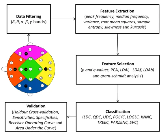
Figure 1 shows the processes used in the methodology to process the data, that include filtering, feature extraction, feature selection, classification and finally validation.
Figure 1: Methodology data processes
Each of these processes is discussed in more detail below. Figure 1 shows a data science methodology that produces a robust data analytics based solution.
4.1.1 Data Pre-processing
In the CHB-MIT database, each record was sampled at 256Hz, with 16-bit resolution. Signals were recorded simultaneously through twenty-three different channels, via 19 electrodes and a ground attached to the surface of the scalp.
A bandpass filter was applied to each of the 342 EEG segments (171 seizures, 171 non-seizures) to extract the EEG data in each of the frequency blocks. Second order Butterworth filters were used as they offer good transition band characteristics at low coefficient orders; thus, they can be implemented efficiently. This results in five columns of additional data; the complete bandwidth (0.5-30Hz), delta (δ: 0.5 ≤ f ≤ 4 Hz), theta (θ: 4 ≤ f ≤ 8 Hz), alpha (α: 8 ≤ f ≤ 12 Hz): and beta (β: 12 ≤ f ≤ 25 Hz). In other words, each block contains 115 columns of data for each of the 23 EEG channels in the original data (N=23*(complete bandwidth+delta+theta+alpha+beta) = 23*5=115).
4.1.2 Feature Selection
The feature vectors in this paper are generated from the 171 seizure files and 171 non-seizure blocks, obtained from 23 patients, using peak frequency, median frequency, variance, root mean squares, sample entropy, skewness and kurtosis. These features were extracted from each of the 115 columns in an EEG block (N=7 features * 115 columns = 805). The literature reports that median frequency, sample entropy and root mean square have the most potential to discriminate between seizure and non-seizure records. To validate these findings, the discriminant capabilities of each feature are determined using several measures: statistical
Data Filtering ( Feature Extraction ( Feature Selection ( Classification ( Validation (
significance (p and q-values), principal component analysis (PCA) – Principle Component one (PC1) and Principle Component two (PC2), linear discriminant analysis independent search (LDAi), linear discriminant analysis forward search (LDAf), linear discriminant analysis backward search (LDAb) and gram-schmidt (GS) analysis.
Using these measures, the top 20 uncorrelated features were extracted from all regions of the EEG scalp readings (region-by-region feature extraction is considered later in the paper). For example, in the case of p-values we select the top 20 uncorrelated features (from the 805 features that we have) that have the highest p-values and use these features with all our classifiers. The tttest2 function in Matlab can be used to extract p-values and they can be ranked using the sort function. These features are then used to determine determine which classifier performs the best. The same approach is used for the q-values. The mafdr function in Matlab can be used to determine the q-values and again, they can be ranked using the sort function. In the case of principle component one (PC1), the top 20 uncorrelated features that comprise the most variance in PC1 were selected and evaluated against all classifiers. The same approach was used for PC2. In the case of linear discriminant analysis feature selection, the featseli, featself, and featselb provided by the Matlab pattern recognition toolbox PRTools is used to provide an ordered ranking of features. In a similar way, the Gram-Schmidt ranks and orders each feature by importance.
Table 3 shows that the best results were obtained from the linear discriminant analysis backward search technique with an area under the curve (AUC) of 91%. This was followed closely by statistical p and q-values with AUC values of 90% and 89% respectively.
AUCs for Feature Selection techniques
knnc knnc svn knnc tree knnc loglc knnc loglc
p q PC1 PC2 PC1 2 LDAi LDAf LDAb GS
90 89 83 88 87 86 88 91 88
Sensitivities for Feature Selection techniques
knnc knnc svn knnc treec knnc loglc knnc loglc
p q PC1 PC2 PC1&2 LDAi LDAf LDAb GS
83 84 53 86 80 78 76 84 76
Specificities for Feature Selection techniques
knnc knnc svn knnc treec knnc loglc knnc loglc
p q PC1 PC2 PC1& 2 LDAi LDAf LDAb GS
83 82 90 81 79 80 85 85 86
Table 3: Results for Feature Selection Techniques
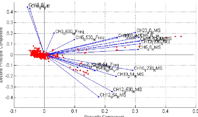
Figure 2 shows (using PCA) that several RMS and median frequency features, from different channels and frequency bands, appear along the principal component. This is consistent with the findings in [47]–[49]. The vertical axis shows that CH12_48_Var, CH9_48_Var, and CH3_0530_MFreq features align closest with the second principal component. Again, these results are consistent with the findings in [47]–[49].
Figure 2: PCA for Median Frequency and RMS Feature Discrimination
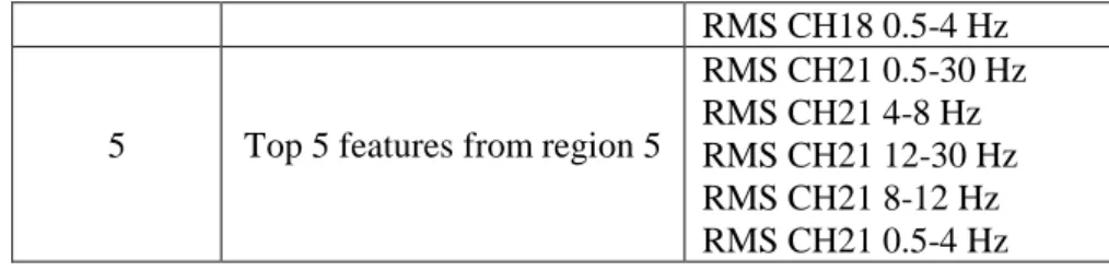
This study also extracts the top five uncorrelated features from each of the five regions covered by the EEG scalp electrodes as shown in Table 4. . This ensures that each region is represented without the bias from all other regions, and allows classifiers to detect focal seizures in different parts of the brain. The features extracted, using the generalised and region-by-region approach, are used to evaluate the capabilities of several classifiers considered in this study and are
Feature set Description Features
1 Top 5 features from region 1
RMS CH2 0.5-30 Hz Samp Entropy CH2 0.5-4 Hz RMS CH2 4-8 Hz RMS CH2 0.5-4 Hz Samp Entropy CH1 0.5-4 Hz
2 Top 5 features from region 2
RMS CH16 0.5-30 Hz RMS CH16 0.5-4 Hz RMS CH12 12-30 Hz RMS CH16 12-30 Hz RMS CH16 4-8 Hz
3 Top 5 features from region 3
RMS CH3 0.5-30 Hz RMS CH3 0.5-4 Hz RMS CH4 4-8 Hz Med Freq CH3 0.5-4 Hz RMS CH4 0.5-30 Hz
4 Top 5 features from region 4
RMS CH18 4-8 Hz RMS CH18 0.5-30 Hz RMS CH17 0.5-30 Hz RMS CH17 0.5-4 Hz
RMS CH18 0.5-4 Hz
5 Top 5 features from region 5
RMS CH21 0.5-30 Hz RMS CH21 4-8 Hz RMS CH21 12-30 Hz RMS CH21 8-12 Hz RMS CH21 0.5-4 Hz Table 4: Top five features for the five scalp regions
The top five features per region were selected based on their rank determined by the linear discriminant backward search technique, creating five feature sets containing five features each. The top 20 uncorrelated features and the 25 region-by-region features are compared in the evaluation.
4.1.4 Classification
Following an analysis of the literature, the study in this paper adopts simple, yet powerful algorithms. These include the linear discriminant classifier (LDC), quadratic discriminant classifier (QDC), uncorrelated normal density based classifier (UDC), polynomial classifier (POLYC), logistic classifier (LOGLC), k-nearest neighbour (KNNC), decision tree (TREEC), parzen classifier (PARZENC) and the support vector machine (SVC) [62].
4.1.5 Validation Methods
In order to determine the overall accuracy of each of the classifiers several validation techniques have been considered. These include Holdout Cross-validation, Sensitivities, Specificities, Receiver Operating Curve (ROC) and Area Under the Curve (AUC). The Holdout Cross-Validation technique uses 80 percent of randomly selected observations (N=19.2) to train the algorithms and 20 percent of randomly selected test cases to test the algorithms (N=3.8).
5. EVALUATION
5.1 Results Using Top Twenty Uncorrelated Features Ranked Using LDA Backward Search Feature Selection
In the first evaluation, the top twenty uncorrelated features, extracted from each of the frequency bands within each of the EEG channels, and nine classifiers are used. The performance for each classifier is evaluated using the sensitivity, specificity, mean error, standard deviation and AUC values with 100 simulations and randomly selected training and testing sets for each simulation. In this study, high sensitivities are important to ensure that seizures can be detected within an alarm system. High specificities are considered equally important as high false alarm rates (more than 1 per hour) will deter doctors from using it.
5.1.1 Classifier Performance
The first evaluation uses all the seizure and non-seizure blocks from all subjects in the CHB-MIT dataset (171 seizures and 171 non-seizures). The simulations use 80% for training and 20% for testing. Table 4, shows the mean averages obtained over 100 simulations for the sensitivity, specificity, and AUC.
QDC 65% 92% 62% UDC 39% 95% 65% POLYC 70% 83% 83% LOGLC 79% 86% 89% KNNC 84% 85% 91% TREEC 78% 80% 86% PARZENC 61% 86% 54% SVC 79% 86% 88%
Table 4: Classifier Performance Results for Top 20 Uncorrelated Features
As shown in Table 4, the sensitivities (seizure), in this initial test, are low for all classifiers. This is interesting given that the dataset is balanced between seizure and non-seizure blocks. One possible reason for this is that the ictal length across the 171 records was 60 seconds. However, in the CHB-MIT records ictal periods ranged between 2 and 752 (cut down to 60 seconds) seconds. It is possible that some ictal blocks resemble non-seizure records resulting in misclassification (particularly blocks that contain 2 seconds of ictal data). However, given that 64% of the ictal blocks contain more than 30 seconds of icta data, this is appropriate for training. Furthermore, it is a decision that is supported by the relatively high sensitivity, specificity and AUC values. Nonetheless, further investigation is required. Table 5 shows the error and standard deviations obtained over 100 iterations.
80% Holdout: 100 Repetitions Classifier Err SD LDC 0.23 0.05 QDC 0.21 0.04 UDC 0.32 0.04 POLYC 0.23 0.05 LOGLC 0.17 0.04 KNNC 0.15 0.04 TREEC 0.20 0.05 PARZENC 0.26 0.04 SVC 0.17 0.04
Table 5: Cross Validation Results for top 20 Uncorrelated Features
The results show that all techniques are able to achieve a classification error, lower than the base-rate error of 50% (i.e. 171/342).
5.1.2 Model Selection
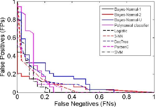
The receiver operator characteristic (ROC) curve shows the cut-off values for the false negative and false-positive rates. Figure 3 indicates that several of the classifiers performed reasonably well. The AUC values in Table 4 support these findings with good accuracy values for the LOGLC and KNNC classifiers.
Figure 3: Received Operator Curve for top 20 Uncorrelated Features
5.2 Results Using Top Five Uncorrelated Features Ranked Using LDA Backward Search Feature Selection from Five Head Regions
In the second evaluation, the top five uncorrelated features, extracted from five main regions across the head, are used to determine whether the detection of seizures can be improved. Again, the performance for each classifier is evaluated using the sensitivity, specificity, mean error, standard deviation and AUC values with 100 simulations and randomly selected training and testing sets for each simulation.
5.2.1 Classifier Performance
The simulations use 80% for training and 20% for testing. As shown in Table 6, the sensitivities (seizure), for most of the algorithms have improved, including the specificities values. The AUC results also show improvements for several of the classifiers, with 93% achieved by the KNNC classifier. From the previous results, we find a 4% increase in sensitivities, a 3% increase in specificities and a 2 % increase in the performance of the KNNC classifier, with other classifiers improving by similar values.
Classifier Sensitivity Specificity AUC
LDC 78% 88% 55% QDC 84% 86% 60% UDC 51% 91% 70% POLYC 78% 88% 89% LOGLC 82% 84% 90% KNNC 88% 88% 93% TREEC 82% 81% 89% PARZENC 81% 93% 61% SVC 85% 86% 90%
Table 6: Classifier Performance Results from Top five Uncorrelated Features from Five Head Regions
Again, the results in Table 7 show that the mean error has decreased by 3% using the holdout technique. This indicates that using a region-by-region approach is better at discriminating between seizure and non-seizure events.
80% Holdout: 100 Repetitions Classifier Err SD LDC 0.16 0.04 QDC 0.14 0.04 UDC 0.29 0.04 POLYC 0.16 0.04 LOGLC 0.17 0.04 KNNC 0.12 0.03 TREEC 0.18 0.05 PARZENC 0.13 0.04 SVC 0.14 0.03
Table 7 Cross Validation Results from top five Uncorrelated Features from Five Regions Overall, the mean errors produced, using all of the validation techniques, are significantly lower than the expected error, which is 171/342, i.e. 50%.
5.2.2 Model Selection
Again, the ROC curve shows the cut-off values for the false-negative and false-positive rates. Figure 4 indicates that the performance of several classifiers improved. The AUC values in Table 6 support these findings with the KNNC classifier showing a 2% increase in performance.
Figure 4: Received Operator Curve for top five Uncorrelated Features from Five Head Regions
6. DISCUSSION
The study has focused on discriminating between seizure and non-seizure EEG records across a group of 23 subjects, rather than a single individual. The classifiers are trained using all 24 cases, and therefore, classification is generalised across the whole population contained in the CHB-MIT database. To achieve this, features from all the channels that capture the EEG in all parts of the brain were used. In the initial classification results, the top 20 uncorrelated features from the whole of the head (not region-by-region) were extracted from 805 possible features. This was determined using the linear discriminant analysis backward search technique to rank features. This approach achieved reasonably good results, using the KNNC classifier, with 84% for sensitivity, 85% for specificity, 91% for the AUC, with a global error of 15%.
Interestingly, the features used in this initial evaluation, involved channels from the four lobes of the brain, occipital, parietal, frontal, and temporal, but not the channels spread across the centre of the head. This implied that rather than having generalised seizures across the whole of the brain, a majority of focal seizures occurred in each of the lobes. Unlike studies that used the BONN dataset, which only contains one channel; or the FRE dataset, that contains six channels and identifies focal and extra focal channels; the CHB-MIT database used in this study contains 23 channels with no information on the seizure type or location.
Using the top five uncorrelated features from EEG channels specific to the five main regions of the head improved the sensitivities and specificities, while producing high AUC values. The best classification algorithm was again the KNNC classifier, which achieved 88% for sensitivity, 88% for specificity, and an AUC value of 93% with a 12% global error. This was followed closely by the SVC classifier, which achieved 85% for sensitivity, 86% for specificity, and an AUC value of 90% with a 14% global error.
Comparing our results with other studies, we find that Shoeb [18] produced a better sensitivity value (96%) than those reported in this study. However, their approach utilised a SVM classifier trained and tested on an individual patient and was not concerned with the generalisation of seizures across a bigger population group. Consequently, the 88% sensitivity value produced in this paper appears to be extremely good given that our classifiers were trained and tested on data from 23 different patients, not just one. In a similar study, Nasehi et al. [20] used a neural network and reported a sensitivity value of 98%, which again is higher than the results reported in this study. However, as with the work of Shoeb, the classifiers were trained and tested on specific patients.
In comparison with other studies that adopted a similar approach to our study, our approach produced better overall results. For instance, in [19] Khan et al. report a 83.6% specificity value, while Patel et al. [31] report 94% for sensitivity, 77.9% for specificity, and 87.7% for overall accuracy. Yuan et al. [63] report 91.72% for sensitivity, 94.89% for specificity, and 94.9% for accuracy. While Aarabi et al. [64], Nicolaou et al. [30], Kannathal et al. [50], and Patnaik et al. [30] all reported similar results. The results found in this paper can be compared in more detail with the papers listed in Table 8.
Author Year Data set Classifier Patients Sens (%) Spec (%) Acc (%) FPR/h
Acharya et al. [25] 2012 BONN PNN, SVM, C4.5, BC, FSC, KNN, GMM 10 94.4-99.4 91.1-100 88.1-95.9 - Bao et al. [65] 2008 BONN PNN 10 - - 71-96.8 - Chandaka et al. [66] 2009 BONN SVM 10 92.00 100 95.96 - Kannathal et al. [50] 2005 BONN ANFIS 10 91.49 93.02 92.2 - Kumar et al. [67] 2010 BONN EN, RBNN 10 - - 94.5 - Kumari and Jose [68] 2011 BONN SVM 5 100.00 100 100 0 Nicolaou and Georgiou [22] 2012 BONN SVM 10 94.38 93.23 80.9-86.1 - Polat and Gunes [69] 2007 BONN DTC 10 99.40 99.31 98.72 - Polat and Gunes [26] 2008 BONN C4.5 10 99.49 99.12 99.32 - Song and Lio
[70] 2010 BONN BPNN, ELM 10 97.26 98.77 95.67 - Srinivasan et al. [21] 2007 BONN PNN, EN - - 100 Subasi [71] 2007 BONN MPNN, ME 10 95.00 94 94.5 - Subasi and Gursoy [72] 2010 BONN SVM 99-100 98.5-100 98.75-100 - Ubeyli [23] 2008 BONN SVM 10 99.25 100 99.3 - Ubeyli [24] 2009 BONN PNN, SVM, MPNN, CNN, ME, MME, RNN 10 99.20 99.78 99.2 - Yuan et al.[73] 2011 BONN SVM, BPNN, ELM 10 92.50 96 96 -
Zheng et al.
[74] 2012 BXH SVM 7 44.23 - - 1.6-10.9
Khan et al. [19] 2012 CHBMIT LDA 5 83.60 100 91.8 Nasehi and Pourghassem [20] 2013 CHBMIT IPSONN 23 98.00 - - 0.125 Shoeb [18] 2009 CHBMIT SVM 24 96.00 - - 0.08 Acir and Guzelis [32] 2004 DEU SVM 7 90.30 - - Rasekhi et al. [33] 2013 EUR SVM 10 73.90 - - 0.15
Park et al. [29] 2011 FRE SVM 18 92.5-97.5 - - 0.2-0.29 Patel et al. [31] 2009 FRE SVM, LDA, QDA, MDA 21 90.9-94.2 59.5-77.9
76.5-87.7 - Patnaik and
Manyam [30] 2008 FRE BPNN 21 91.29 99.19 - -
Williamson et
al. [28] 2011 FRE SVM 21 90.80 - - 0.094
Yuan et al. [63] 2012 FRE ELM 21 93.85 94.89 94.9 0.35
Bao et al. [65] 2009 JPH PNN 12 - - 94.07 - Saab and Gotman [75] 2005 MON BC 76.00 - - 0.34 Grewal and Gotman [76] 2005 MON2 BC 16 89.40 - - 0.22 D’Alessandro et al. [77] 2005 PEN & BON PNN 2 100.00 - - 1.1 Sorensen et al. [78] 2010 RIG SVM 6 77.8-100 - - 0.16-5.31 Gandhi et al.[71] 2011 SGR & BONN PNN, SVM 21 + 10 - - 99.9 - D’Alessandro et al.[26] 2003 Unknown PNN 4 62.50 90.47 - 0.2775 Subasi [79] 2006 Unknown DFNN 5 93.10 92.8 93.1 -
Table 8: Seizure detection studies and classification results
This work has potential future clinical applications in the investigation of patients with suspected seizure disorders and may be useful in the assessment of patients with non-epileptic attack disorder (NEAD). Introducing automated seizure detection technologies could help increase capacity within healthcare systems such as the UKs National Health Service (NHS), which currently suffers from a chronic shortage of trained clinical neurophysiologists to interpret EEGs. Tele-EEG reporting has previously been suggested as a solution and more recently online systems [80], [81], which are interesting approaches, but carry increased costs and concerns over data security. Nonetheless, these, including automated seizure detection may be viable solutions, following further work aimed at improving accuracy further.
7. CONCLUSIONS AND FUTURE WORK
Within a supervised-learning paradigm, this study has addressed this challenge by utilising EEG signals to classify seizure and non-seizure records. Our approach posits a new method for generalising seizure detection across different subjects without prior knowledge about the focal point of seizures. Our results show an improvement on existing studies with 88% for sensitivity, 88% for specificity and 93% for the area under the curve, with a 12% global error, using the k-NN classifier.
The results suggest that the algorithms in-situ with existing clinical systems and practices may enable clinicians to make a diagnosis of epilepsy and instigate treatment earlier. It can help to reduce costs by limiting the number of trained specialists required to perform the interpretation by automating the detection of correlates of seizure activity generalised across different regions of the brain and across multiple subjects.
There are a large number of features reported in the literature, which have not been considered in this paper. In particular our future work will consider the set of features described in [82] and [83]. Furthermore, our future work will investigate the use of more advanced machine learning algorithms, despite the good performance of the classifiers considered in this paper. In particular, we will investigate the use of convolutional neural networks [84] and SVM with different kernels [85].
Window sizes will also be considered to determine whether further improvements on accuracies can be made. Future development will also utilise regression analysis and a larger number of observations. This may help to define the characteristics of the pre-ictal phase. In addition, more advanced classification algorithms, and techniques, will be considered, including advanced artificial neural network architectures (higher order and spiking neural networks). The investigation and comparison, of features, such as fractal dimension and cepstrum analysis, autocorrelation zero crossing and correlation dimension, has also not been performed. These techniques should be investigated in a head-to-head comparison, with linear methods.
The paper has investigated the use of classic yet powerful machine learning algorithms and evaluated their ability to detect correlates of seizure activity. While the results are convincing
approach evaluates the algorithms using offline data, however, this is not a good indicator of the system’s ability as the signals that are used to train and test the algorithms are processed and cleaned and appropriate features extracted. This is a major concern and our future work will look to implement the methodology pipeline using real-time signals, using advances in the Internet of Things and Big Data community that currently utilise data processing technologies, such as Apache Spark.
Finally, there are concerns regarding the verification of the results produced using the CHB-MIT dataset against other datasets. Our future work will investigate the use of a bigger dataset, using patients provided by our co-author from The Walton Centre NHS Foundation Trust, and other datasets that permit access to verify the findings in this paper.
Overall, the study demonstrates that classification algorithms provide an interesting line of enquiry, when separating seizure and non-seizure records.
REFERENCES
[1] S. Fazel, A. Wolf, N. Langstrom, C. R. Newton, and P. Lichtenstein, “Premature mortality in epilepsy and the role of psychiatric comorbidity: a total population study,” Lancet, vol. 382, no. 9905, pp. 1646–54, 2013.
[2] J. Engel, Seizures and Epilepsy. 2013, p. 736.
[3] W. A. Chaovalitwongse, R. S. Pottenger, W. Shouyi, F. Ya-Ju, and L. D. Iasemidis, “Pattern- and Network-Based Classification Techniques for Multichannel Medical Data Signals to Improve Brain Diagnosis,” IEEE Trans. Syst. Man Cybern., vol. 41, no. 5, pp. 977–988, 2011.
[4] T. Maiwald, M. Winterhalder, R. Aschenbrenner-Scheibe, H. U. Voss, A. Shulze-Bonhage, and J. Timmer, “Comparison of three nonlinear seizure prediction methods by means of the seizure prediction characteristic,” Phys. D Nonlinear Phenom., vol. 194, pp. 357–368, 2004.
[5] P. R. Carney, S. Myers, and J. D. Deyer, “Seizure Prediction: Methods,” Epilepsy Behav., vol. 22, pp. S94–S101, 2011.
[6] F. Mormann, R. G. Andrzejak, C. E. Elgar, and K. Lehnertz, “Seizure prediction the long and winding road,” Brain, vol. 130, pp. 314–333, 2007.
[7] L. Ayoubian, H. Lacoma, and J. Gotman, “Automatic seizure detection in SEEG using high frequency activities in wavelet domain,” Med. Eng. Phys., vol. 35, no. 3, pp. 319– 328, 2013.
[8] R. Hopfengartner, B. S. Kasper, W. Graf, S. Gollwitzer, G. Kreiselmeyer, H. Stefan, and H. Hamer, “Automatic seizure detection in long-term scalp EEG using an adaptive thresholding technique: A validation study for clinical routine.,” J. Int. Fed. Clin. Neurophysiol., vol. 125, no. 7, pp. 1346–1352, 2014.
[9] B. Hunyadi, M. Signoretto, W. Van Paesschen, J. Suykens, S. Van Huffel, and M. De Vos, “Incorporating structural information from the multichannel EEG improves patient-specific seizure detection,” Clin. Neurophysiol., vol. 123, no. 12, pp. 2352–61, 2012.
[10] J. Yoo, L. Yan, D. El-Demak, M. Altaf, A. H. Shoeb, and A. P. Chandrakasan, “An 8-Channel Scalable EEG Acquisition SoC with Fully Integrated Patient-Specific Seizure Classification and Recorder Processor,” IEEE J. Solid State Circuits, vol. 49, no. 9, pp. 214–228, 2013.
[11] M. A. B. Altaf, J. Tilak, Y. Kifle, and J. Yoo, “A 1.83µJ/classification nonlinear support-vector-machine-based patient-specific seizure classification SoC,” in IEEE International Solid-State Circuits Conference, 2013, pp. 100–102.
[12] J. Gotman, J. R. Ives, and P. Gloor, “Automatic recognition of inter-ictal epileptic activity in prolonged EEG recordings,” Electroencephalogr. Clin. Neurophysiol., vol. 46, no. 5, pp. 510–520, 1979.
[13] D. J. Koffler and J. Gotman, “Automatic Detection of Spike and wave bursts in ambulatory EEG recordings,” Electroencephalogr. Clin. Neurophysiol., vol. 61, no. 2, pp. 165–180, 85AD.
[14] J. Gotman, “Automatic recognition of epileptic seizures in the EEG,” Electroencephalogr. Clin. Neurophysiol., vol. 54, no. 5, pp. 530–540, 1982.
[15] J. Gotman, “Automatic detection of seizures and spikes,” J. Clin. Neurophysiol., vol. 16, no. 2, pp. 130–140, 199AD.
[16] H. Qu and J. Gotman, “Improvement in seizure detection performance by automatic adaptation to the EEG of each patient,” Clin. Neurophysiol., vol. 86, no. 2, pp. 79–87, 1993.
[17] R. Lopes, J. M. Lina, F. Fahoum, and J. Gotman, “Detection of epileptic activity in fMRI without recording the EEG,” NuroImage, vol. 60, no. 3, pp. 1867–1879, 2012. [18] A. H. Shoeb, “Application of Machine Learning to Epileptic Seizure Onset and
Treatment,” 2009.
[19] Y. U. Khan, N. Rafiuddin, and O. Farooq, “Automated Seizure Detection in Scalp EEG Using Multiple Wavelet Scales,” in IEEE International Conference on Signal Processing, Computing and Control, 2012, pp. 1–5.
[20] S. Nasehi and H. Pourghassem, “Patient Specific Epileptic Seizure Onset Detection Algorithm Based on Spectral Features and IPSONN Classifier,” in International Conference on Communication Systems and Network Technologies (CSNT), 2013, pp. 186–190.
[22] N. Nicalaou and J. Georgiou, “Detection of Epileptic Electroencephalogram based on Permutation Entropy and Support Vector Machines,” Expert Syst. Appl., vol. 39, pp. 202–209, 2012.
[23] E. D. Ubeyli, “Analysis of EEG signals by combining eigenvector methods and multiclass support vector machines,” Comput. Biol. Med., vol. 200, pp. 10–27, 2008. [24] E. D. Ubeyli, “Decision Support Systems for Time-Varying Biomedical Signals: EEG
Signal Classification,” Expert Syst. Appl., vol. 36, pp. 2275–2284, 2009.
[25] U. R. Acharya, F. Molinari, S. V. Sree, S. Chattopadhyay, K. H. Ng, and J. S. Suri, “Automated Diagnosis of Epileptic EEG Using Entropies,” Biomed. Signal Process. Control, vol. 7, pp. 401–408, 2012.
[26] K. Polat and S. Gunes, “A novel Data Reduction Method: Distance Based Data Reduction and its Applicaiton to Classification of Epileptiform EEG Signals,” Appl. Math. Comput., vol. 200, pp. 10–27, 2008.
[27] Q. Yuan, W. Zhou, Y. Liu, and J. Wang, “Epileptic EEG Detection with Linear and Nonlinear Features,” Epilepsy Behav., vol. 24, pp. 415–421, 2012.
[28] J. R. Williamson, D. W. Bliss, and D. W. Browne, “Epileptic seizure prediction using the spatiotemporal correlation structure of intracranial EEG,” in International Conference on Acoustics, Speech and Signal Processing, 2011, pp. 665–668.
[29] Y. Park, L. Luo, K. K. Parhi, and T. Netoff, “Seizure prediction with spectral power of EEG using cost-sensitive support vector machines,” Epilepsia, vol. 52, pp. 1761–1770, 2011.
[30] L. M. Patnaik and O. K. Manyam, “Epileptic EEG detection using neural networks and post-classification,” Comput. Methods Programs Biomed., vol. 91, pp. 100–109, 2008. [31] K. Patel, C. Chem-Pin, S. Fau, and C. J. Bleakley, “Low power real-time seizure
detection for ambulatory EEG,” in 3rd International Conference on Pervasive Computing Technologies for Healthcare, 2009, pp. 1–7.
[32] N. Acir and C. Guzelis, “Automatic spike detection in EEG by a two-stage procedure based on support vector machines,” Comput. Biol. Med., vol. 34, pp. 561–575, 2004. [33] J. Rasekhi, M. R. K. Mollaei, M. Bandarabadi, C. A. Teixeira, and A. Dourado,
“Preprocessing effects of 22 linear univariate features on the performance of seizure prediction methods,” J. Neurosci. Methods, vol. 217, pp. 9–16, 2013.
[34] M. Libenson, Practical Approach to Electroencephalography. 2009, p. 464.
[35] B. Moslem, B. Karlsson, M. O. Diab, M. Khalil, and C. Marque, “Classification Performance of the Frequency-Related Parameters Derived from Uterine EMG Signals,” in International Conference of the IEEE Engineering in Medicine and Biology Society, 2011, pp. 3371–4.
[36] W. L. Maner and R. E. Garfield, “Identification of human term and preterm labor using artificial neural networks on uterine electromyography data.,” Ann. Biomed. Eng., vol. 35, no. 3, pp. 465–73, Mar. 2007.
[37] M. Hassan, J. Terrien, C. Marque, and B. Karlsson, “Comparison between Approximate Entropy, Correntropy and Time Reversibility: Application to Uterine Electromyogram Signals,” Med. Eng. Phys., vol. 33, no. 8, pp. 980–6, 2011.
[38] C. Buhimschi, M. B. Boyle, G. R. Saade, and R. E. Garfield, “Uterine activity during pregnancy and labor assessed by simultaneous recordings from the myometrium and abdominal surface in the rat.,” Am. J. Obstet. Gynecol., vol. 178, no. 4, pp. 811–22, Apr. 1998.
[39] H. Leman, C. Marque, and J. Gondry, “Use of the electrohysterogram signal for characterization of contractions during pregnancy.,” IEEE Trans. Biomed. Eng., vol. 46, no. 10, pp. 1222–9, Oct. 1999.
[40] C. K. Marque, J. Terrien, S. Rihana, and G. Germain, “Preterm labour detection by use of a biophysical marker: the uterine electrical activity.,” BMC Pregnancy Childbirth, vol. 7 Suppl 1, p. S5, Jan. 2007.
[41] M. O. Diab, A. El-Merhie, N. El-Halabi, and L. Khoder, “Classification of Uterine EMG signals using Supervised Classification method,” Biomed. Sci. Eng., vol. 3, no. 9, pp. 837–842, 2010.
[42] P. Carre, H. Leman, C. Fernandez, and C. Marque, “Denoising of the Uterine EHG by an Undecimated Wavelet Transform,” IEEE Trans. Biomed. Eng., vol. 45, no. 9, pp. 1104–13, 1998.
[43] W. L. Maner, L. B. MacKay, G. R. Saade, and R. E. Garfield, “Characterization of abdominally acquired uterine electrical signals in humans, using a non-linear analytic method.,” Med. Biol. Eng. Comput., vol. 44, no. 1–2, pp. 117–23, Mar. 2006.
[44] W. L. Maner, R. E. Garfield, H. Maul, G. Olson, and G. Saade, “Predicting term and preterm delivery with transabdominal uterine electromyography,” Obstet. Gynecol., vol. 101, no. 6, pp. 1254–1260, Jun. 2003.
[45] S. Sanei and J. A. Chambers, EEG Signal Processing. 2007, p. 312.
[46] A. Aarabi, Fazel-Rezai., and Y. Aghakhani, “A fuzzy rule-based system for epileptic seizure detection in intracranial EEG,” Clin. Neurophysiol., vol. 120, no. 9, pp. 1648– 1657, 2009.
[47] W. Ning and M. R. Lyu, “Exploration of instantaneous amplitude and frequency features for epileptic seizure prediction,” in 12th IEEE International Conference on Bioinformatics and Bioengineering, 2012, pp. 292–297.
[49] A. A. Abdul-latif, I. Cosic, D. K. Kimar, and B. Polus, “Power changes of EEG signals associated with muscle fatigue: the root mean square analysis of EEG bands,” in IEEE Proceedings of Intelligent Sensors, Sensor Networks and Information Processing Conference,, 2004, pp. 531–534.
[50] N. Kannathal, M. L. Choo, U. R. Acharya, and P. K. Sadasivan, “Entropies for detection of epilepsy in EEG,” Comput. Methods Programs Biomed., vol. 81, no. 2, pp. 187–194, 2005.
[51] B. R. Greene, S. Faul, W. P. Marnane, G. Lightbody, I. Korotchikova, and G. B. Boylan, “A comparison of quantitative EEG features fro neonatal seizure detection,” Clin. Neurophysiol., vol. 119, no. 6, pp. 1248–1261, 2008.
[52] L. Diambra, J. C. B. de Figueiredo, and C. P. Malta, “Epileptic activity recognition in EEG recording,” Phys. A Statical Mech. its Appl., vol. 273, no. 3–4, pp. 495–505, 1999.
[53] K. M. Kelly, D. S. Shiau, R. T. Kern, J. H. Chien, M. C. K. Yang, K. A. Yandora, J. P. Valeriano, J. J. Halford, and J. C. Sackellares, “Assessment of a scalp EEG-based automated seizure detection system,” Clin. Neurophysiol., vol. 121, no. 11, pp. 1832– 1843, 2010.
[54] L. D. Iasemidis, “Epileptic seizure prediction and control,” IEEE Trans. Biomed. Eng., vol. 50, no. 5, pp. 549–558, 2003.
[55] I. Omerhodzic, S. Avdakovic, A. Nuhanovic, and K. Dizdarevic, “Energy distribution of EEG signals: EEG signal wavelet-neural network classifier,” World Acad. Sci. Eng. Technol., vol. 37, pp. 1240–1245, 2010.
[56] T. Gandhi, B. K. Panigrahi, and S. Anand, “A comparative study of wavelet families for EEG signal classification,” Neurocomputing, vol. 74, no. 17, pp. 3051–3057, 2011. [57] B. Litt and J. Echauz, “Prediction of Epileptic seizures,” Lancet Neurol., vol. 1, no. 1,
pp. 22–30, 2002.
[58] U. R. Acharya, S. V. Stee, G. Swapna, R. J. Martis, and J. S. Suri, “Automated EEG analysis of epilepsy: A review,” Knowledge-Based Syst., vol. 45, no. June, pp. 147– 165, 2013.
[59] A. Aarabi and B. He, “A rule-based seizure prediction method for focal neocortical epilepsy,” Clin. Neurophysiol., vol. 123, no. 6, pp. 1111–1122, 2012.
[60] H. Adeli, S. Ghosh-Dastidar, and N. Dadmehr, “A Wavelet-Chaos Methodology for Analyssi of EEGs and EEG subbands to detect seizure and epilepsy,” IEEE Trans. Biomed. Eng., vol. 54, no. 2, pp. 205–211, 2007.
[61] A. Aarabi, R. Fazel-Rezai, and Y. Aghakhani, “EEG Seizure Prediction: Measures and challenges,” in Annual International Conference of the IEEE in Engineering in Medicine and Biology, 2009, pp. 1864–1867.
[62] F. van der Heijde, R. P. W. Duin, D. de Ridder, and D. M. J. Tax, Classification, Parameter Estimation and State Estimation. 2005, p. 440.
[63] Q. Yuan, W. Zhou, Y. Liu, and J. Wang, “Epileptic seizure detection with linear and nonlinear features,” Epilepsy Behav., vol. 24, no. 4, pp. 415–421, 2012.
[64] A. Aarabi, F. Wallois, and R. Grebe, “Automated neonatal seizure detection: a multistage classification system through feature selection based on relevance and redundancy analysis,” Clin. Neurophysiol., vol. 117, no. 2, pp. 328–340, 2006.
[65] F. S. Bao, D. Y. C. Lie, and Y. Zhang, “A New Approach to Automated Epileptic Diagnosis using EEG and Probabilisitic Neural Network,” in 20th IEEE International Conference on Tools with Artificial Intellligence, 2008.
[66] S. Chandaka, A. Chatterjee, and S. Munshi, “Cross-correlation aided support vector machine classifier for classification,” Expert Syst. Appl., vol. 36, pp. 1329–1336, 2009. [67] S. P. Kumar, N. Sriraam, P. G. Benakop, and B. C. Jinaga, “Entropies based detection of epileptic seizures with artificial neural network classifiers,” Expert Syst. Appl., vol. 37, no. 4, pp. 3284–3291, 2010.
[68] R. S. S. Kumari and P. Jose, “Seizure detection in EEG using time frequency analysis and SVM,” in International Conference on Emerging Trends in Electrical and Computer Technology, 2011, pp. 626–630.
[69] K. Polat and S. Gunes, “Classification of epileptiform EEG using a hybrid system based on decision tree classifier and fast Fourier Transform,” Appl. Math. Comput., vol. 187, pp. 1017–1026, 2007.
[70] Y. Song and P. Lio, “A new approach for epileptic seizure detection: sample entropy based feature extractionadn extreme learning machine,” J. Biomed. Sci. Eng., vol. 3, p. 556, 2010.
[71] A. Subasi, “EEG Signal Classification using Wavelet Feature Extraction and a Mixture of Expert Model,” Expert Syst. Appl., vol. 32, pp. 1084–1093, 2007.
[72] A. Subasi and M. I. Gursoy, “EEG Signal Classification using PCA, ICA, LDA and Support Vector Machines,” Expert Syst. Appl., vol. 37, pp. 8659–8666, 2010.
[73] Q. Yuan, W. Zhou, S. Li, and D. Cai, “Epileptic EEG classification based on extreme learning machine and nonlinear features,” Epilepsy Res., vol. 96, no. 1–2, pp. 29–38, 2011.
[74] Z. G. Zheng, Y. Liutao, F. Yuwei, H. Zhuyi, C. Lisheng, Z. Shouwen, W. Dahui, and H. Zhangang, “Seizure prediction model based on method of common spatial patterns and support vector machine,” in International Conference on Information Science and Technology, 2012, pp. 29–34.
[76] S. Grewal and J. Gotman, “An automatic warning system for epileptic seizures recorded on intrcerbral EEGs,” Clin. Neurophysiol., vol. 116, pp. 2460–2472, 2005. [77] M. D’Alessandro, G. Vachtsevanos, R. . Esteller, J. Echauz, S. Cranstoun, G. Worrell,
L. Parish, and B. Litt, “A Multi-feature and multi-channel univariate selection process for seizure prediction,” Clin. Neurophysiol., vol. 116, pp. 506–516, 2005.
[78] T. L. Sorensen, U. L. Olsen, I. Conradsen, J. Hendriksen, T. W. Kjaer, C. E. Thomsen, and H. B. D. Sorensen, “Automatic epileptic seizure onset detection using Matching Pursuit: A Case Study,” in International Conference on Engineering in Medicine and Biology Society, 2010, pp. 3277–3280.
[79] A. Subasi, “Automatic detection of eipileptic seizure using dynamic fuzzy neural networks,” Expert Syst. Appl., vol. 31, pp. 320–328, 2006.
[80] F. Furbass, P. Ossenblok, M. Hartmann, H. Perko, A. M. Skupch, G. Lindinger, L. Elezi, and E. Pataraia, “Prospective Multi-Center Study of an Automatic Online Seizure Detection System for Epilepsy Monitoring Units,” Clin. Neurophysiol., vol. In Press, 2014.
[81] R. Meier, H. Dittrich, A. Schulze-Bonhage, and A. Aertsen, “Detecting epileptic seizures in long-term human EEG: A new approach to automatic online and real-time detection and classification of polymorphic seizure patterns,” Clin. Neurophysiol., vol. 25, no. 3, pp. 119–131, 2008.
[82] L. Logesparan, A. J. Casson, and E. Rodriquez-Villegas, “Optimal features for online seizure detection,” Med. Biol. Eng. Comput., vol. 50, no. 7, pp. 659–669, 2012.
[83] L. Logesparan, A. J. Casson, S. A. Imtiaz, and Rodriquez-Villegas, “Discriminating between best performing features for seizure detection and data selection,” in The 35th IEEE Annual International Conference on Engineering in Medicine and Biology Society, 2013, pp. 1692–1695.
[84] Y. Ren and Y. Wu, “Convolutional deep belief networks for feature extraction of EEG signal,” in International Joint Conference on Neural Networks, 2014, pp. 2850–2853. [85] C. H. Seng, R. Demirli, L. Khuon, and D. Bolger, “Seizure detection in EEG signals
using support vector machines,” in The 28th IEEE Annual Northeast Bioengineering Conference, 2012, pp. 231–232.