On the Optimality of Classifier Chain for
Multi-label Classification
Weiwei Liu Ivor W. Tsang∗
Centre for Quantum Computation and Intelligent Systems University of Technology, Sydney
[email protected], [email protected]
Abstract
To capture the interdependencies between labels in multi-label classification prob-lems,classifier chain(CC) tries to take the multiple labels of each instance into account under a deterministic high-order Markov Chain model. Since its perfor-mance is sensitive to the choice of label order, the key issue is how to determine the optimal label order for CC. In this work, we first generalize the CC model over a random label order. Then, we present a theoretical analysis of the generaliza-tion error for the proposed generalized model. Based on our results, we propose
adynamic programming based classifier chain(CC-DP) algorithm to search the
globally optimal label order for CC and agreedy classifier chain(CC-Greedy) algorithm to find a locally optimal CC. Comprehensive experiments on a num-ber of real-world multi-label data sets from various domains demonstrate that our proposed DP algorithm outperforms state-of-the-art approaches and the CC-Greedy algorithm achieves comparable prediction performance with CC-DP.
1
Introduction
Multi-label classification, where each instance can belong to multiple labels simultaneously, has significantly attracted the attention of researchers as a result of its various applications, ranging from document classification and gene function prediction, to automatic image annotation. For example, a document can be associated with a range of topics, such asSports,FinanceandEducation[1]; a gene belongs to the functions ofprotein synthesis,metabolismandtranscription[2]; an image may have bothbeachandtreetags [3].
One popular strategy for multi-label classification is to reduce the original problem into many bina-ry classification problems. Many works have followed this strategy. For example, binabina-ry relevance (BR) [4] is a simple approach for multi-label learning which independently trains a binary classifier for each label. Recently, Dembczynski et al. [5] have shown that methods of multi-label learn-ing which explicitly capture label dependency will usually achieve better prediction performance. Therefore, modeling the label dependency is one of the major challenges in multi-label classifica-tion problems. Many multi-label learning models [5, 6, 7, 8, 9, 10, 11, 12] have been developed to capture label dependency. Amongst them, theclassifier chain(CC) model is one of the most popular methods due to its simplicity and promising experimental results [6].
CC works as follows: One classifier is trained for each label. For the(i+ 1)th label, each instance is augmented with the 1st, 2nd,· · ·,ith label as the input to train the(i+ 1)th classifier. Given a new instance to be classified, CC firstly predicts the value of the first label, then takes this instance together with the predicted value as the input to predict the value of the next label. CC proceeds in this way until the last label is predicted. However, here is the question: Does the label order affect the performance of CC?Apparently yes, because different classifier chains involve different
classifiers trained on different training sets. Thus, to reduce the influence of the label order, Readet al.[6] proposed theensembled classifier chain(ECC) to average the multi-label predictions of CC over a set of random chain ordering. Since the performance of CC is sensitive to the choice of label order, there is another important question: Is there any globally optimal classifier chain which can achieve the optimal prediction performance for CC?If yes,how can the globally optimal classifier chain be found?
To answer the last two questions, we first generalize the CC model over a random label order. We then present a theoretical analysis of the generalization error for the proposed generalized model. Our results show that the upper bound of the generalization error depends on the sum of reciprocal of square of the margin over the labels. Thus, we can answer the second question: the globally optimal CC exists only when the minimization of the upper bound is achieved over this CC. To find the globally optimal CC, we can search overq! different label orders1, whereq denotes the
number of labels, which is computationally infeasible for a largeq. In this paper, we propose the
dynamic programming based classifier chain(CC-DP) algorithm to simplify the search algorithm,
which requiresO(q3nd)time complexity. Furthermore, to speed up the training process, agreedy
classifier chain(CC-Greedy) algorithm is proposed to find a locally optimal CC, where the time
complexity of the CC-Greedy algorithm isO(q2nd).
Notations: Assume xt ∈ Rd is a real vector representing an input or instance (feature) for t ∈
{1,· · ·, n}.ndenotes the number of training samples.Yt⊆ {λ1, λ2,· · ·, λq}is the corresponding
output (label). yt ∈ {0,1}q is used to represent the label setYt, whereyt(j) = 1if and only if
λj∈ Yt.
2
Related work and preliminaries
To capture label dependency, Hsuet al. [13] first use compressed sensing technique to handle the multi-label classification problem. They project the original label space into a low dimensional label space. A regression model is trained on each transformed label. Recovering multi-labels from the regression output usually involves solving a quadratic programming problem [13], and many works have been developed in this way [7, 14, 15]. Such methods mainly aim to use different projection methods to transform the original label space into another effective label space.
Another important approach attempts to exploit the different orders (first-order, second-order and high-order) of label correlations [16]. Following this way, some works also try to provide a proba-bilistic interpretation for label correlations. For example, Guo and Gu [8] model the label correla-tions using a conditional dependency network; PCC [5] exploits a high-order Markov Chain model to capture the correlations between the labels and provide an accurate probabilistic interpretation of CC. Other works [6, 9, 10] focus on modeling the label correlations in a deterministic way, and CC is one of the most popular methods among them. This work will mainly focus on the deterministic high-order classifier chain.
2.1 Classifier chain
Similar to BR, theclassifier chain(CC) model [6] trainsqbinary classifiershj (j ∈ {1,· · ·, q}).
Classifiers are linked along a chain where each classifierhjdeals with the binary classification
prob-lem for labelλj. The augmented vector{xt,yt(1),· · · ,yt(j)}nt=1 is used as the input for training
classifierhj+1. Given a new testing instancex, classifierh1in the chain is responsible for
predict-ing the value ofy(1)using inputx. Then,h2predicts the value ofy(2)takingxplus the predicted
value ofy(1)as an input. Following in this way,hj+1predictsy(j+ 1)using the predicted value
ofy(1),· · ·,y(j)as additional input information. CC passes label information between classifiers, allowing CC to exploit the label dependence and thus overcome the label independence problem of BR. Essentially, it builds a deterministic high-order Markov Chain model to capture the label correlations.
1!
2.2 Ensembled classifier chain
Different classifier chains involve different classifiers learned on different training sets and thus the order of the chain itself clearly affects the prediction performance. To solve the issue of selecting a chain order for CC, Readet al.[6] proposed the extension of CC, calledensembled classifier chain
(ECC), to average the multi-label predictions of CC over a set of random chain ordering. ECC first randomly reorders the labels{λ1, λ2,· · · , λq}many times. Then, CC is applied to the reordered
labels for each time and the performance of CC is averaged over those times to obtain the final prediction performance.
3
Proposed model and generalization error analysis
3.1 Generalized classifier chainWe generalize the CC model over a random label order, calledgeneralized classifier chain(GCC) model. Assume the labels{λ1, λ2,· · · , λq}are randomly reordered as{ζ1, ζ2,· · ·, ζq}, whereζj=
λkmeans labelλkmoves to positionjfromk. In the GCC model, classifiers are also linked along
a chain where each classifierhjdeals with the binary classification problem for labelζj(λk). GCC
follows the same training and testing procedures as CC, while the only difference is the label order. In the GCC model, for inputxt,yt(j) = 1if and only ifζj∈ Yt.
3.2 Generalization error analysis
In this section, we analyze the generalization error bound of the multi-label classification problem using GCC based on the techniques developed for the generalization performance of classifiers with a large margin [17] and perceptron decision tree [18].
LetXrepresent the input space. Boths and¯sare msamples drawn independently according to an unknown distributionD. We denote logarithms to base 2 bylog. If S is a set,|S|denotes its cardinality. ∥ · ∥means thel2 norm. We train a support vector machine(SVM) for each labelζj.
Let{xt}nt=1as the feature and{yt(ζj)}nt=1as the label, the output parameter of SVM is defined as
[wj, bj] =SV M({xt,yt(ζ1),· · · ,yt(ζj−1)}nt=1,{yt(ζj)}nt=1). The margin for labelζj is defined
as:
γj = 1
||wj||2
(1) We begin with the definition of the fat shattering dimension.
Definition 1([19]). LetHbe a set of real valued functions. We say that a set of pointsP isγ -shattered byHrelative tor= (rp)p∈P if there are real numbersrpindexed byp∈Psuch that for
all binary vectorsbindexed byP, there is a functionfb∈ Hsatisfying
fb(p) =
{
≥rp+γ ifbp= 1
≤rp−γ otherwise
The fat shattering dimensionf at(γ)of the setHis a function from the positive real numbers to the integers which maps a valueγto the size of the largestγ-shattered set, if this is finite, or infinity otherwise.
AssumeHis the real valued function class andh∈ H. l(y, h(x))denotes the loss function. The expected error of his defined as erD[h] = E(x,y)∼D[l(y, h(x))], where(x, y) drawn from the
unknown distributionD. Here we select 0-1 loss function. So,erD[h] = P(x,y)∼D(h(x) ̸= y).
ers[h]is defined asers[h] = n1
n
∑
t=1
[yt̸=h(xt)].2
SupposeN(ϵ,H,s)is theϵ-covering number ofHwith respect to thel∞pseudo-metric measuring the maximum discrepancy on the samples. The notion of the covering number can be referred to the Supplementary Materials. We introduce the following general corollary regarding the bound of the covering number:
2
Corollary 1([17]). LetHbe a class of functionsX →[a, b]andDa distribution overX. Choose
0< ϵ <1and letd=f at(ϵ/4)≤em. Then
E(N(ϵ,H,s))≤2
(4m(b−a)2
ϵ2
)dlog(2em(b−a)/(dϵ))
(2)
where the expectationEis over sampless∈Xmdrawn according toDm.
We study the generalization error bound of the specified GCC with the specified number of labels and margins. LetGbe the set of classifiers of GCC,G = {h1, h2,· · ·, hq}. ers[G]denotes the fraction of the number of errors that GCC makes ons. Defineˆx∈X× {0,1},hˆj(ˆx) =hj(x)(1−
y(j))−hj(x)y(j). If an instancex∈Xis correctly classified byhj, thenˆhj(ˆx)<0. Moreover, we
introduce the following proposition:
Proposition 1. If an instancex∈Xis misclassified by a GCC model, then∃hj ∈G,ˆhj(ˆx)≥0.
Lemma 1. Given a specified GCC model withqlabels and with marginsγ1, γ2,· · · , γq for each label satisfyingki = f at(γi/8), wheref at is continuous from the right. If GCC has correctly
classifiedmmulti-labeled examplessgenerated independently according to the unknown (but fixed) distributionDand¯sis a set of anothermmulti-labeled examples, then we can bound the following probability to be less thanδ:P2m{s¯s:∃a GCC model, it correctly classifiess, fraction of¯s
misclas-sified> ϵ(m, q, δ)}< δ, whereϵ(m, q, δ) =m1(Qlog(32m) + log2δq)andQ=∑qi=1kilog(8emk
i ). Proof. (of Lemma 1). SupposeGis a GCC model withqlabels and with marginsγ1, γ2,· · ·, γq, the probability event in Lemma 1 can be described as
A={s¯s:∃G, ki=f at(γi/8), ers[G] = 0, er¯s[G]> ϵ}.
Letˆsandˆ¯sdenote two different set ofm examples, which are drawn i.i.d. from the distribution D× {0,1}. Applying the definition ofxˆ, ˆhand Proposition 1, the event can also be written as A ={ˆsˆ¯s : ∃G,γˆi = γi/2, ki =f at(ˆγi/4), ers[G] = 0, ri =maxtˆhi(ˆxt),2ˆγi =−ri,|{ˆy ∈ˆ¯s :
∃hi ∈ G,hˆi(yˆ) ≥ 2ˆγi+ri}| > mϵ}.Here,−maxthˆi(xˆt)means the minimal value of|hi(x)|
which represents the margin for labelζi, so2ˆγi =−ri. Letγki =min{γ′ :f at(γ′/4) ≤ki}, so
γki ≤γˆ
i, we define the following function:
π(ˆh) = 0 ifˆh≥0 −2γki ifˆh≤ −2γki ˆ h otherwise soπ(ˆh)∈[−2γki,0]. Letπ( ˆG) ={π(ˆh) :h∈G}. LetBki
ˆsˆ¯s represent the minimalγki-cover set ofπ( ˆG)in the pseudo-metricdˆsˆ¯s. We have that for anyhi ∈ G, there existsf˜∈ Bˆskˆ¯si,|π(ˆhi(ˆz))−π( ˜f(ˆz))| < γki, for allˆz∈ˆsˆ¯s. For allxˆ∈ˆs, by
the definition ofri,ˆhi(ˆx) ≤ ri = −2ˆγi, andγki ≤ γˆ
i,ˆh
i(ˆx) ≤ −2γki,π(ˆhi(ˆx)) = −2γki, so
π( ˜f(ˆx))<−2γki+γki=−γki. However, there are at leastmϵpointsˆy∈ˆ¯ssuch thatˆhi(yˆ)≥0,
soπ( ˜f(ˆy))>−γki > maxtπ( ˜f(ˆxt)). Sinceπonly reduces separation between output values, we
conclude that the inequalityf˜(ˆy)> maxtf˜(ˆxt)holds. Moreover, themϵpoints inˆ¯swith the largest
˜
f values must remain for the inequality to hold. By the permutation argument, at most2−mϵof the
sequences obtained by swapping corresponding points satisfy the conditions for fixedf˜. As for anyhi ∈ G, there exists f˜ ∈ Bˆskˆ¯si, so there are|B
ki
ˆsˆ¯s| possibilities off˜that satisfy the inequality forki. Note that |Bˆskˆ¯si|is a positive integer which is usually bigger than 1 and by the union bound, we get the following inequality:
P(A)≤(E(|Bk1 ˆsˆ¯s|) +· · ·+E(|B kq ˆsˆ¯s|))2 −mϵ≤(E(|Bk1 ˆsˆ¯s |)× · · · ×E(|B kq ˆsˆ¯s |))2 −mϵ
Since every set of pointsγ-shattered byπ( ˆG)can beγ-shattered byGˆ, sof atπ( ˆG)(γ)≤f atGˆ(γ),
whereGˆ={hˆ:h∈G}. Hence, by Corollary 1 (setting[a, b]to[−2γki,0],ϵtoγkiandmto2m),
E(|Bki
ˆsˆ¯s|) =E(N(γki, π( ˆG),ˆsˆ¯s))≤2(32m)
dlog(8em
whered = f atπ( ˆG)(γki/4) ≤ f atGˆ(γki/4) ≤ ki. ThusE(|B ki ˆsˆ¯s|) ≤ 2(32m) kilog(8kiem), and we obtain P(A)≤(E(|Bk1 ˆsˆ¯s|)× · · · ×E(|B kq ˆsˆ¯s|))2 −mϵ≤ q ∏ i=1 2(32m)kilog(8emki )= 2q(32m)Q whereQ=∑qi=1kilog(8emk i ). And so(E(|B k1 ˆsˆ¯s |)× · · · ×E(|B kq ˆsˆ¯s |))2 −mϵ< δprovided ϵ(m, q, δ)≥ 1 m ( Qlog(32m) + log2 q δ ) as required.
Lemma 1 applies to a particular GCC model with a specified number of labels and a specified margin for each label. In practice, we will observe the margins after running the GCC model. Thus, we must bound the probabilities uniformly over all of the possible margins that can arise to obtain a practical bound. The generalization error bound of the multi-label classification problem using GCC is shown as follows:
Theorem 1. Suppose a randommmulti-labeled sample can be correctly classified using a GCC model, and suppose this GCC model contains qclassifiers with margins γ1, γ2,· · ·, γq for each label. Then we can bound the generalization error with probability greater than1−δto be less than
130R2
m (
Q′log(8em) log(32m) + log2(2m)
q
δ )
whereQ′=∑qi=1(γ1i)2 andRis the radius of a ball containing the support of the distribution. Before proving Theorem 1, we state one key Symmetrization lemma and Theorem 2.
Lemma 2(Symmetrization). LetHbe the real valued function class. sand¯saremsamples both drawn independently according to the unknown distributionD. Ifmϵ2≥2, then
Ps( sup
h∈H|
erD[h]−ers[h]| ≥ϵ) ≤ 2Ps¯s( sup
h∈H|
er¯s[h]−ers[h]| ≥ϵ/2) (3)
The proof details of this lemma can be found in the Supplementary Material.
Theorem 2([20]). LetHbe restricted to points in a ball ofM dimensions of radiusRabout the origin, then f atH(γ)≤min {R2 γ2,M + 1 } (4)
Proof. (of Theorem 1). We must bound the probabilities over different margins. We first use
Lem-ma 2 to bound the probability of error in terms of the probability of the discrepancy between the performance on two halves of a double sample. Then we combine this result with Lemma 1. We must consider all possible patterns ofki’s for labelζi. The largest value ofkiism. Thus, for fixedq,
we can bound the number of possibilities bymq. Hence, there aremqof applications of Lemma 1.
Letci={γ1, γ2,· · ·, γq}denote thei-th combination of margins varied in{1,· · ·, m}q.Gdenotes
a set of GCC models. The generalization error ofGcan be represented aserD[G]anders[G]is 0, whereG∈ G. The uniform convergence bound of the generalization error is
Ps(sup G∈G| erD[G]−ers[G]| ≥ϵ) Applying Lemma 2, Ps(sup G∈G |erD[G]−ers[G]| ≥ϵ)≤2Ps¯s(sup G∈G |er¯s[G]−ers[G]| ≥ϵ/2) LetJci ={s¯s: ∃a GCC modelGwithqlabels and with marginsci :ki =f at(γ
i/8), ers[G] = 0, er¯s[G]≥ϵ/2}. Clearly, Ps¯s(sup G∈G| er¯s[G]−ers[G]| ≥ϵ/2)≤Pm q( mq ∪ i=1 Jci )
Aski still satisfieski = f at(γi/8), Lemma 1 can still be applied to each case ofPm
q
(Jci). Let
δk=δ/mq. Applying Lemma 1 (replacingδbyδk/2), we get:
Pmq(Jci)< δk/2
whereϵ(m, k, δk/2) ≥2/m(Qlog(32m) + log2×2
q
δk )andQ=
∑q
i=1kilog(4emki ). By the union
bound, it suffices to show thatPmq(∪mq i=1Jci)≤ ∑mq i=1P mq(J ci)< δk/2×m q =δ/2. Applying Lemma 2, Ps(sup G∈G| erD[G]−ers[G]| ≥ϵ)≤2Ps¯s(sup G∈G| er¯s[G]−ers[G]| ≥ϵ/2) ≤2Pmq (mq ∪ i=1 Jci ) < δ
Thus,Ps(supG∈G|erD[G]−ers[G]| ≤ ϵ) ≥ 1−δ. LetRbe the radius of a ball containing the support of the distribution. Applying Theorem 2, we getki = f at(γi/8) ≤ 65R2/(γi)2. Note
that we have replaced the constant82 = 64by65in order to ensure the continuity from the right
required for the application of Lemma 1. We have upperboundedlog(8em/ki)bylog(8em). Thus,
erD[G]≤2/m ( Qlog(32m) + log2(2m) q δ ) ≤ 130R2 m (
Q′log(8em) log(32m) + log2(2m)
q
δ ) whereQ′=∑qi=1 1
(γi)2.
Given the training data size and the number of labels, Theorem 1 reveals one important factor in re-ducing the generalization error bound for the GCC model: the minimization of the sum of reciprocal of square of the margin over the labels. Thus, we obtain the following Corollary:
Corollary 2(Globally Optimal Classifier Chain). Suppose a randommmulti-labeled sample with
qlabels can be correctly classified using a GCC model, this GCC model is the globally optimal
classifier chain if and only if the minimization ofQ′ in Theorem 1 is achieved over this classifier chain.
Given the number of labelsq, there areq! different label orders. It is very expensive to find the globally optimal CC, which can minimizeQ′, by searching over all of the label orders. Next, we discuss two simple algorithms.
4
Optimal classifier chain algorithm
In this section, we propose two simple algorithms for finding the optimal CC based on our result in Section 3. To clearly state the algorithms, we redefine the margins with label order information. Given label setM = {λ1, λ2,· · · , λq}, suppose a GCC model containsqclassifiers. Letoi(1 ≤
oi ≤ q)denote the order of λi in the GCC model, γioi represents the margin for label λi, with
previousoi−1labels as the augmented input. Ifoi= 1, thenγi1represents the margin for labelλi,
without augmented input. ThenQ′is redefined asQ′=∑qi=1 1
(γioi)2. 4.1 Dynamic programming algorithm
To simplify the search algorithm mentioned before, we propose the CC-DP algorithm to find the globally optimal CC. Note thatQ′ =∑qi=1 1
(γioi)2 = 1 (γoqq )2 +· · ·+[ 1 (γkok+1+1)2 + ∑k j=1 1 (γjoj)2 ] , we explore the idea of DP to iteratively optimizeQ′over a subset ofMwith the length of1,2,· · ·, q. Finally, we can obtain the optimalQ′ overM. Assumei∈ {1,· · ·, q}. LetV(i, η)be the optimal Q′over a subset ofMwith the length ofη(1≤η≤q), where the label order is ending by labelλi.
SupposeMiηrepresent the corresponding label set forV(i, η). Whenη =q,V(i, q)be the optimal Q′overM, where the label order is ending by labelλi. The DP equation is written as:
V(i, η+ 1) = min j̸=i,λi̸∈Mjη { 1 (γiη+1)2 +V(j, η) } (5)
whereγiη+1 is the margin for labelλi, with M η
j as the augmented input. The initial condition of
DP is: V(i,1) = (γ11
i)2
andMi1={λi}. Then, the optimalQ′overMcan be obtained by solving
mini∈{1,···,q}V(i, q). Assume the training of linear SVM takesO(nd). The CC-DP algorithm is
shown as the following bottom-up procedure: from the bottom, we first computeV(i,1) = (γ11
i)2
, which takesO(nd). Then we computeV(i,2) = minj̸=i,λi̸∈Mj1{
1 (γ2
i)2
+V(j,1)}, which requires at mostO(qnd), and setMi2=Mj1∪ {λi}. Similarly, it takes at mostO(q2nd)time complexity to
calculateV(i, q). Last, we iteratively solve this DP Equation, and usemini∈{1,···,q}V(i, q)to get
the optimal solution, which requires at mostO(q3nd)time complexity.
Theorem 3(Correctness of CC-DP). Q′can be minimized by CC-DP, which means this Algorithm can find the globally optimal CC.
The proof can be referred to in the Supplementary Materials.
4.2 Greedy algorithm
We propose a CC-Greedy algorithm to find a locally optimal CC to speed up the CC-DP algorithm. To save time, we construct only one classifier chain with the locally optimal label order. Based on the training instances, we select the label from{λ1, λ2,· · · , λq}as the first label, if the maximum
margin can be achieved over this label, without augmented input. The first label is denoted byζ1.
Then we select the label from the remainder as the second label, if the maximum margin can be achieved over this label withζ1as the augmented input. We continue in this way until the last label
is selected. Finally, this algorithm will converge to the locally optimal CC. We present the details of the CC-Greedy algorithm in the Supplementary Materials, where the time complexity of this algorithm isO(q2nd).
5
Experiment
In this section, we perform experimental studies on a number of benchmark data sets from different domains to evaluate the performance of our proposed algorithms for multi-label classification. All the methods are implemented in Matlab and all experiments are conducted on a workstation with a 3.2GHZ Intel CPU and 4GB main memory running 64-bit Windows platform.
5.1 Data sets and baselines
We conduct experiments on eight real-world data sets with various domains from three websites.345
Following the experimental settings in [5] and [7], we preprocess the LLog, yahoo art, eurlex sm and eurlex ed data sets. Their statistics are presented in the Supplementary Materials. We compare our algorithms with some baseline methods: BR, CC, ECC, CCA [14] and MMOC [7]. To perform a fair comparison, we use the same linear classification/regression package LIBLINEAR [21] with L2-regularized square hinge loss (primal) to train the classifiers for all the methods. ECC is averaged over several CC predictions with random order and the ensemble size in ECC is set to 10 according to [5, 6]. In our experiment, the running time of PCC and EPCC [5] on most data sets, like slashdot and yahoo art, takes more than one week. From the results in [5], ECC is comparable with EPCC and outperforms PCC, so we do not consider PCC and EPCC here. CCA and MMOC are two state-of-the-art encoding-decoding [13] methods. We cannot get the results of CCA and MMOC on yahoo art 10, eurlex sm 10 and eurlex ed 10 data sets in one week. Following [22], we consider the Example-F1, Macro-F1 and Micro-F1 measures to evaluate the prediction performance of all methods. We perform 5-fold cross-validation on each data set and report the mean and standard error of each evaluation measurement. The running time complexity comparison is reported in the Supplementary Materials. 3 http://mulan.sourceforge.net 4http://meka.sourceforge.net/#datasets 5 http://cse.seu.edu.cn/people/zhangml/Resources.htm#data
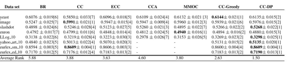
Table 1: Results of Example-F1 on the various data sets (mean±standard deviation). The best results are in bold. Numbers in square brackets indicate the rank.
Data set BR CC ECC CCA MMOC CC-Greedy CC-DP
yeast 0.6076±0.019[6] 0.5850±0.033[7] 0.6096±0.018[5] 0.6109±0.024[4] 0.6132±0.021 [3] 0.6144±0.021[1] 0.6135±0.015[2] image 0.5247±0.025[7] 0.5991±0.021[1] 0.5947±0.015[4] 0.5947±0.009[4] 0.5960±0.012[3] 0.5939±0.021[6] 0.5976±0.015[2] slashdot 0.4898±0.024[6] 0.5246±0.028[4] 0.5123±0.027[5] 0.5260±0.021[3] 0.4895±0.022[7] 0.5266±0.022[2] 0.5268±0.022[1] enron 0.4792±0.017[7] 0.4799±0.011[6] 0.4848±0.014[4] 0.4812±0.024[5] 0.4940±0.016[1] 0.4894±0.016[2] 0.4880±0.015[3] LLog 10 0.3138±0.022[6] 0.3219±0.028[4] 0.3223±0.030[3] 0.2978±0.026[7] 0.3153±0.026[5] 0.3269±0.023[2] 0.3298±0.025[1] yahoo art 10 0.4840±0.023[5] 0.5013±0.022[4] 0.5070±0.020[3] - - 0.5131±0.015[2] 0.5135±0.020[1] eurlex sm 10 0.8594±0.003[5] 0.8609±0.004[1] 0.8606±0.003[3] - - 0.8600±0.004[4] 0.8609±0.004[1] eurlex ed 10 0.7170±0.012[5] 0.7176±0.012[4] 0.7183±0.013[2] - - 0.7183±0.013[2] 0.7190±0.013[1] Average Rank 5.88 3.88 3.63 4.60 3.80 2.63 1.50 5.2 Prediction performance
Example-F1 results for our method and baseline approaches in respect of the different data sets are reported in Table 1. Other measure results are reported in the Supplementary Materials. From the results, we can see that: 1) BR is much inferior to other methods in terms of Example-F1. Our experiment provides empirical evidence that the label correlations exist in many real word data sets and because BR ignores the information about the correlations between the labels, BR achieves poor performance on most data sets. 2) CC improves the performance of BR, however, it underperforms ECC. This result verifies the answer to our first question stated in Section 1: the label order does affect the performance of CC; ECC, which averages over several CC predictions with random order, improves the performance of CC. 3) CC-DP and CC-Greedy outperforms CCA and MMOC. This studies verify that optimal CC achieve competitive results compared with state-of-the-art encoding-decoding approaches. 4) Our proposed CC-DP and CC-Greedy algorithms are successful on most data sets. This empirical result also verifies the answers to the last two questions stated in Section 1: the globally optimal CC exists and CC-DP can find the globally optimal CC which achieves the best prediction performance; the CC-Greedy algorithm achieves comparable prediction performance with CC-DP, while it requires lower time complexity than CC-DP. In the experiment, our proposed algorithms are much faster than CCA and MMOC in terms of both training and testing time, and achieve the same testing time with CC. Through the training time for our algorithms is slower than BR, CC and ECC. Our extensive empirical studies show that our algorithms achieve superior performance than those baselines.
6
Conclusion
To improve the performance of multi-label classification, a plethora of models have been developed to capture label correlations. Amongst them, classifier chain is one of the most popular approaches due to its simplicity and good prediction performance. Instead of proposing a new learning model, we discuss three important questions in this work regarding the optimal classifier chain stated in Section 1. To answer these questions, we first propose a generalized CC model. We then provide a theoretical analysis of the generalization error for the proposed generalized model. Based on our results, we obtain the answer to the second question: the globally optimal CC exists only if the mini-mization of the upper bound is achieved over this CC. It is very expensive to search overq!different label orders to find the globally optimal CC. Thus, we propose the CC-DP algorithm to simplify the search algorithm, which requiresO(q3nd)complexity. To speed up the CC-DP algorithm, we
propose a Greedy algorithm to find a locally optimal CC, where the time complexity of the CC-Greedy algorithm isO(q2nd). Comprehensive experiments on eight real-world multi-label data sets
from different domains verify our theoretical studies and the effectiveness of proposed algorithms. Acknowledgments
This research was supported by the Australian Research Council Future Fellowship FT130100746.
References
[1] Robert E. Schapire and Yoram Singer. BoosTexter: A Boosting-based System for Text Categorization.
[2] Zafer Barutc¸uoglu and Robert E. Schapire and Olga G. Troyanskaya. Hierarchical multi-label prediction of gene function. Bioinformatics, 22(7):22–7, 2006.
[3] Matthew R. Boutell and Jiebo Luo and Xipeng Shen and Christopher M. Brown. Learning Multi-Label Scene Classification.Pattern Recognition, 37(9):1757–1771, 2004.
[4] Grigorios Tsoumakas and Ioannis Katakis and Ioannis P. Vlahavas. Mining Multi-label Data. InData Mining and Knowledge Discovery Handbook, pages 667–685, 2010. Springer US.
[5] Krzysztof Dembczynski and Weiwei Cheng and Eyke H¨ullermeier. Bayes Optimal Multilabel Classifi-cation via Probabilistic Classifier Chains. Proceedings of the 27th International Conference on Machine Learning, pages 279–286, Haifa, Israel, 2010. Omnipress.
[6] Jesse Read and Bernhard Pfahringer and Geoffrey Holmes and Eibe Frank. Classifier Chains for Multi-label Classification. InProceedings of the European Conference on Machine Learning and Knowledge Discovery in Databases: Part II, pages 254–269, Berlin, Heidelberg, 2009. Springer-Verlag.
[7] Yi Zhang and Jeff G. Schneider. Maximum Margin Output Coding.Proceedings of the 29th International Conference on Machine Learning, pages 1575–1582, New York, NY, 2012. Omnipress.
[8] Yuhong Guo and Suicheng Gu. Multi-Label Classification Using Conditional Dependency Networks.
Proceedings of the Twenty-Second International Joint Conference on Artificial Intelligence, pages 1300– 1305, Barcelona, Catalonia, Spain, 2011. AAAI Press.
[9] Sheng-Jun Huang and Zhi-Hua Zhou. Multi-Label Learning by Exploiting Label Correlations Locally.
Proceedings of the Twenty-Sixth AAAI Conference on Artificial Intelligence, Toronto, Ontario, Canada, 2012. AAAI Press.
[10] Feng Kang and Rong Jin and Rahul Sukthankar. Correlated Label Propagation with Application to Multi-label Learning. 2006 IEEE Computer Society Conference on Computer Vision and Pattern Recognition, pages 1719–1726, New York, NY, 2006. IEEE Computer Society.
[11] Weiwei Liu and Ivor W. Tsang. Large Margin Metric Learning for Multi-Label Prediction.Proceedings of the Twenty-Ninth Conference on Artificial Intelligence, pages 2800–2806, Texas, USA, 2015. AAAI Press.
[12] Mingkui Tan and Qinfeng Shi and Anton van den Hengel and Chunhua Shen and Junbin Gao and Fuyuan Hu and Zhen Zhang. Learning Graph Structure for Multi-Label Image Classification via Clique Genera-tion. The IEEE Conference on Computer Vision and Pattern Recognition, 2015.
[13] Daniel Hsu and Sham Kakade and John Langford and Tong Zhang. Multi-Label Prediction via Com-pressed Sensing. Advances in Neural Information Processing Systems, pages 772–780, 2009. Curran Associates, Inc.
[14] Yi Zhang and Jeff G. Schneider. Multi-Label Output Codes using Canonical Correlation Analysis. Pro-ceedings of the Fourteenth International Conference on Artificial Intelligence and Statistics, pages 873– 882, Fort Lauderdale, USA, 2011. JMLR.org.
[15] Farbound Tai and Hsuan-Tien Lin. Multilabel Classification with Principal Label Space Transformation.
Neural Computation, 24(9):2508–2542, 2012.
[16] Min-Ling Zhang and Kun Zhang. Multi-label learning by exploiting label dependency. Proceedings of the 16th ACM SIGKDD International Conference on Knowledge Discovery and Data Mining, pages 999–1008, QWashington, DC, USA, 2010. ACM.
[17] John Shawe-Taylor and Peter L. Bartlett and Robert C. Williamson and Martin Anthony. Structural Risk Minimization Over Data-Dependent Hierarchies.IEEE Transactions on Information Theory, 44(5):1926– 1940, 1998.
[18] Kristin P. Bennett and Nello Cristianini and John Shawe-Taylor and Donghui Wu. Enlarging the Margins in Perceptron Decision Trees. Machine Learning, 41(3):295–313, 2000.
[19] Michael J. Kearns and Robert E. Schapire. Efficient Distribution-free Learning of Probabilistic Concept-s. Proceedings of the 31st Symposium on the Foundations of Computer Science, pages 382–391, Los Alamitos, CA, 1990. IEEE Computer Society Press.
[20] Peter L. Bartlett and John Shawe-Taylor. Generalization Performance of Support Vector Machines and Other Pattern Classifiers. Advances in Kernel Methods - Support Vector Learning, pages 43–54, Cam-bridge, MA, USA, 1998. MIT Press.
[21] Rong-En Fan and Kai-Wei Chang and Cho-Jui Hsieh and Xiang-Rui Wang and Chih-Jen Lin. LIBLIN-EAR: A Library for Large Linear Classification. Journal of Machine Learning Research, 9:1871–1874, 2008.
[22] Qi Mao and Ivor Wai-Hung Tsang and Shenghua Gao. Objective-Guided Image Annotation. IEEE Transactions on Image Processing, 22(4):1585–1597, 2013.