ECLogger: Cross-Project Catch-Block Logging
Prediction Using Ensemble of Classifiers
Sangeeta Lal∗, Neetu Sardana∗, Ashish Sureka∗∗
∗Jaypee Institute of Information Technology, Noida, Uttar-Pradesh, India ∗∗ABB Corporate Research, Bangalore, India
[email protected], [email protected], [email protected] Abstract
Background: Software developers insert log statements in the source code to record program execution information. However, optimizing the number of log statements in the source code is challenging. Machine learning based within-project logging prediction tools, proposed in previous studies, may not be suitable for new or small software projects. For such software projects, we can use cross-project logging prediction.
Aim:The aim of the study presented here is to investigate cross-project logging prediction methods and techniques.
Method:The proposed method is ECLogger, which is a novel, ensemble-based, cross-project, catch-block logging prediction model. In the research We use 9 base classifiers were used and combined using ensemble techniques. The performance of ECLogger was evaluated on on three open-source Java projects: Tomcat, CloudStack and Hadoop.
Results:ECLoggerBagging, ECLoggerAverageVote, and ECLoggerMajorityVote show a considerable improvement in the average Logged F-measure (LF) on 3, 5, and 4 source→target project pairs,
respectively, compared to the baseline classifiers. ECLoggerAverageVoteperforms best and shows improvements of 3.12% (averageLF) and 6.08% (averageACC– Accuracy).
Conclusion:The classifier based on ensemble techniques, such as bagging, average vote, and majority vote outperforms the baseline classifier. Overall, the ECLoggerAverageVotemodel performs best. The results show that the CloudStack project is more generalizable than the other projects.
Keywords: classification, debugging, ensemble logging, machine learning, source code analysis, tracing
1. Introduction
Logging is an important software development practice that is typically performed by inserting log statements in the source code. Logging helps to trace the program execution. In the case of failure, software developers can use this tracing information to debug the source code. Logging is important because this is often the only infor-mation available to the developers for debugging because of problems in recreating the same exe-cution environment or because of unavailability of the input used (security/privacy concerns of the user). Logging statements have many applica-tions, such as debugging [1] workload modelling
[2], performance problem diagnosis [3], anomaly detection [4], test analysis [5,6], and remote issue resolution [7].
Source code logging is important, but it has a trade-off between the cost and the benefit [8–11]. Excessive logging in the source code can cause performance and cost overhead. It can also decrease the benefits of logging by generating too many trivial logs, which can potentially make debugging more difficult by hiding important debugging information. Excessive logging can also cause a severe performance bottleneck for a system. In a recent blog, inefficient logging was considered to be a major factor for Tomcat performance problems [12]. Similarly to
exces-sive logging, sparse logging is also problematic. Sparse logging can make logging ineffective by missing important debugging information. Shang et al. [13] reported an experience from a user who was complaining about sparse logging of catch-blocks in Hadoop. Hence, it is important to optimize the number of logging statements in the source code. However, previous research shows that optimizing log statements in the source code is challenging, and developers often face difficul-ties with this task [8–11].
Several recent studies have proposed tools and techniques to help developers optimize log statements in the source code by automatically predicting the code constructs that need to be logged [8, 10, 11]. These techniques learn a pre-diction model from the history of the project (applying supervised learning from annotated training data) to predict logging on new code constructs. Predicting logged code constructs will work well if a sufficient amount of training data is available to train the model. However, many real-world open-source and closed-source applications and new or small projects do not have sufficient prior training data to con-struct the prediction model. There are sev-eral long-lived and large projects that have collected massive amounts of data. One can use training data from these project(s) (source project(s)) to predict logging on a particular project (target project) of interest, i.e. one can perform cross-project logging prediction. Cross-project prediction is also called transfer learning, which consists of transferring predictive models trained from one project (source project) to another project (target project). Cross-project logging prediction can have several benefits: 1) multiple projects can be used for training the model, and hence, good practices can be learned from many projects, and 2) the model can be refined offline over a period of time to improve the performance of logging predic-tion.
Cross-project logging prediction is an impor-tant and a technically challenging task. There are two main challenges in cross-project log-ging prediction: 1) vocabulary mis-match prob-lems and 2) differences in the domain of
nu-merical attributes. The vocabulary mis-match problem can arise due to the use of different terms in the source code of different projects. For example, the Tomcat project has 119 unique exception types, whereas the Hadoop project has 265 unique exception types. Our analysis of these exception types shows that 193 excep-tion types present in the Hadoop project do not exist in the Tomcat project. Similarly, the do-main of numerical attributes may not be the same in different projects. For example, the av-erage SLOC of try-blocks associated with logged catch-blocks is 6.98 and 10.65 for the Tomcat and CloudStack projects, respectively. Hence, it is important to create a prediction model that uses generalized properties for cross-project logging prediction rather than domain-specific properties.
In this paper, the Authors proposeECLogger, a cross-project, catch-block logging prediction framework that addresses the aforementioned challenges. To address the first challenge (vo-cabulary mis-match problem), ECLogger per-forms data standardization prior to learning the model. Data standardization helps to nor-malize the data in a specific range and hence helps to address the problem of data het-erogeneity [14]. To address the second chal-lenge (non-uniform distribution of numerical at-tributes problem), ECLogger, uses an ensem-ble of classifiers-based approach. Ensemensem-ble-based techniques capture the strength of multiple base classifiers [15]. In this work, 9 base clas-sifiers (AdaBoostM1, ADTree, Bayesian network, decision table, J48, logistic regression, Naïve Bayes, random forest and radial basis func-tion network) were used. ECLogger combines these algorithms with three ensemble techniques, i.e. bagging, average vote and majority vote. 8 ECLoggerBagging, 466 ECLoggerAverageVoteand 466 ECLoggerMajorityVote models, i.e. a total of 940 models are created. The performance of ECLogger on three large and popular open-source Java projects: Tomcat, CloudStack and Hadoo-pare evaluated. The experimental results reveal that ECLoggerBagging, ECLoggerAverageVote and ECLoggerMajorityVote show maximum improve-ments of 4.6%, 7.04% and 5.39% in the logged
F-measure, respectively, compared to the baseline classifier.
2. Related work and novel research contributions
In this section, previous works closely related to the study presented in this paper are discussed. They are organized and presented in multiple lines of research. Then the novel research contri-butions of this work in the context of existing work is presented.
2.1. Logging applications
Log statements present in the source code generate log messages at the time of software execution. Log statements and log messages were widely used in the past for different purposes [3,5–7,13,16–18]. Shang et al. [13] used log statements present in a file to predict defects. Shang et al. proposed various product and process metrics using log statements to predict post-release defects. Na-garaj et al. [3] used good and bad logs of the system to detect performance issues in the system. Nagaraj et al. [3] developed a tool, DISTALYZER, that helps developers in finding components re-sponsible for poor system performance. Xu et al. [18] worked on mining console logs from a dis-tributed system at Google to find anomalies in the system. Yuan et al. [17] used log informa-tion to find the root cause of a failure. Yuan et al. developed a tool, SherLog, that can use log information to find information about failed runs without any re-execution of the code. Log messages are also helpful in fixing bugs, as the empirical study performed by Yuan et al. [1] showed that bug reports consisting of log mes-sages were fixed 2.2 times faster compared to bug reports not consisting of log messages. Log messages are also useful in test analysis [5, 6], remote issue resolution [7], security monitoring [19], anomaly detection [4, 18], and usage analy-sis [20]. Many tools have also been proposed to gather log messages [21, 22]. Our work is comple-mentary to these studies, focuses on improving logging in the catch-blocks, and can be
benefi-cial for studies that work on analysing the log information.
2.2. Logging code analysis and improvement
Logging statements are very important in soft-ware development (refer to subsection 2.1), and hence, logging improvements have attracted at-tention from many researchers in the software engineering community [1, 8–11, 17, 23, 24]. Yuan et al. [25] performed a study to identify a set of generic exception types that cause most of the system failures. Yuan et al. [25] proposed a con-servative approach to log all of the generic excep-tion types. Fu et al. [8] studied the logging prac-tices of developers on C# projects and reported the five most frequently logged code constructs. Zhu et al. [11] and Fu et al. [8] proposed a ma-chine learning-based framework for logging pre-diction of exception-type and return-value-check code snippets on C# projects. Lal et al. [9, 10] proposed a machine learning-based framework for catch-block and if-block logging prediction on Java projects. All three approaches use static features from the source code for logging prediction.
Yuan et al. [24] proposed the LogEnhancer tool to help developers in enhancing the cur-rent log statements. LogEnhancer strategically identifies the variables that need to be logged, and experimental results obtained by Yuan et al. [24] showed that LogEnhancer correctly iden-tifies the logged variables 95% of the time. In another study, Yuan et al. [1] proposed a code clone-based tool to predict the correct verbosity level of log statements. Log statements have an option to assign a verbosity level (e.g. debug, info, or trace) as an indicator of the severity level. An incorrect verbosity level to a log statement can have implications on software debugging and other related aspects [26, 27]. Kabinna et al. [23] performed a prediction on the stability (i.e. how likely a logging statement will be modified) of logging statements. Logging statements that are frequently modified may cause log processing applications to crash, and hence, timely logging stability prediction can be beneficial [23]. Our
work is an extension of the logging prediction studies performed by Fu et al. [8], Zhu et al. [11], and Lal et al. [10]. In contrast to these studies, which perform within-project logging prediction, we emphasize on cross-project logging prediction.
2.3. Machine learning applications in logging
Machine learning has been found to be useful in various software engineering applications, such as logging prediction [8,10,11], performance issue diagnosis [3], defect prediction [28], and clean and buggy commit prediction [29]. Fu et al. [8] and Zhu et al. [11] applied the C4.5/J48 algorithm for logging prediction. Lal et al. [10] applied several other machine learning algorithms. These algorithms are Adaboost (ADA), decision tree, Gaussian Naïve Bayes (GNB),K-nearest neigh-bor (KNN), and random forest (RF)) for log-ging prediction. This article considers J48, ADA, Naïve Bayesian (NB), and RF for cross-project catch-block logging as the experimental results by previous studies [8, 10, 11] show that these algorithms perform better than the others. Ad-ditionally, the logistic regression (LR), Bayesian network (BN), decision table (DT), radial basis function network (RBF), and alternating decision trees (ADT) algorithms are considered in this work. These machine learning algorithms have never been explored for logging prediction but have been found to be useful in other branches of software engineering, such as defect predic-tion [30], software project risk predicpredic-tion [31], and re-opened bug prediction [32]. The selection of these algorithms is not random or arbitrary; rather, algorithms belonging to different domains of classification algorithms were selected, for ex-ample, J48 and ADT are decision tree-based algo-rithms, NB and BN are probabilistic algoalgo-rithms, and RBF is an artificial neural network-based algorithm.
2.4. Ensemble methods
Ensemble methods are learning algorithms that construct a prediction model from a set of base classifiers, and new data points are classified by
taking a vote (weighted) of predictions made by base classifiers [33]. An ensemble consists of base classifiers that are combined in some way to predict the label of the new instance. Any base classification algorithm, such as a neural network, a decision tree or any other machine learning algorithm, can be used to generate the base classifiers from the training data. The gen-eralization ability of an ensemble is typically con-siderably better than that of base classifiers [34]. Ensemble methods can use a single or multiple base classification algorithms [35–38]. Bagging [38], boosting [38], average vote [39], majority vote [39], and stacking [40] are some of the en-semble methods. Previous research shows that ensemble methods are useful in improving the performance of machine learning frameworks in various software engineering applications, such as defect prediction [15], cross-project defect pre-diction [30, 41], and blocking bug prepre-diction [42]. However, ensemble methods have not been ex-plored for cross-project logging prediction. In this work, three ensemble methods are applied, namely, bagging [38], average vote [39] and ma-jority vote [39], to construct the cross-project logging prediction model.
2.5. Cross-project prediction
Cross-project prediction trains the model on one (or more) project(s) to make predictions on an-other project of interest. There are two types of cross-project prediction: supervised and unsuper-vised [43, 44]. The superunsuper-vised techniques have some labelled instances available from the target project, whereas the unsupervised ones have all unlabelled instances fromthe target project. In the literature, cross-project prediction has been applied in various applications, such as defect prediction [14, 30, 41], build co-change predic-tion [45], and sentiment classificapredic-tion [46]. How-ever, cross-project logging prediction is a rela-tively unexplored area, which is theprimary fo-cus of this work. To the best knwoledge of the Authors, only Zhu et al. [11] have performed a basic exploration of cross-project logging pre-diction. This study is different from that of Zhu et al. in many aspects: 1) cross-project
catch-block logging prediction is performed on Java projects, whereas Zhu et al. considered C# projects; 2) a focused and in-depth study is per-formed, whereas Zhu et al.performed only a ba-sic experiment on cross-project logging predic-tion; and 3) an ensemble of classifiers is pro-posed, whereas Zhu et al. only used the J48 classifier [39] for cross-project logging predic-tion.
2.6. Research contributions
In context to related work, this work makes the following novel and unique research contribu-tions.
1. A comprehensive analysis of single classi-fiers is performed for within-project and cross-project logging prediction. Further-more, the performances of single-project and multi-project training models are comapred for cross-project logging prediction (refer to section 6.2).
2. ECLogger, a tool based on an ensemble of machine learning algorithms, is proposed for cross-project catch-block logging prediction on Java projects. ECLogger uses static fea-tures from the source code for cross-project catch-block logging prediction. We create 8 ECLoggerBagging, 466 ECLoggerAverageVote and 466 ECLoggerMajorityVotemodels, i.e. a to-tal of 940 models (refer to section 4).
3. The results of a comprehensive evaluation of ECLogger are presented on three large and popular open-source Java projects: Tomcat, CloudStack and Hadoop. The experimental results demonstrate that ECLogger is effec-tive in improving the performance of the cross-project catch-block logging prediction (refer to section 6.3).
3. Background
In this paper, 9 base machine learning algorithms and three ensemble techniques are proposed. The following subsections provide a brief introduction to each of the 9 machine learning algorithms and the 3 ensemble techniques.
3.1. Machine learning algorithms 3.1.1. AdaBoostMI1 (ADA)
AdaBoostM1 (ADA) [47] is an extension of the simple AdaBoost algorithm for multi-class classi-fication. There are two main steps in the ADA algorithm: boosting and ensemble creation. In the boosting phase, ADA first assigns a weight to each data point present in the database (D). Initially, all the data points are assigned an equal weight. The weights assigned to the data points are updated in subsequent iterations. In each iteration, ADA constructs a prediction model (Mi) by training some base machine learning
algorithm, such as a decision tree or a neural net-work, on a sample (Di) of D. In each iteration,
the error rate of the modelMi is computed, and
the weights of incorrectly classified data points are increased, whereas the weights of correctly classified data points are decreased. Using this strategy, ADA generates k prediction models, i.e.Mi, wherei∈{1,2, . . . , k}. In the ensemble
phase, thek models generated in the boosting phase are linearly combined. For prediction on a new instance, the weighted vote of the predic-tion made by thesek prediction models is taken. ADA is an ensemble based algorithm. However, this work consideres default WEKA [48] implan-tation of ADA as a single classification algorithm in Bagging [38], Average Vote [49] and Majority Vote [49] (without the loss of generality). 3.1.2. Alternating decision tree (ADT)
The alternating decision tree (ADT) [50] is a gen-eralization of the decision tree algorithm for classification. The ADT algorithm constructs a tree-like structure (i.e. ADT tree) for predic-tion. The ADT tree consists of decision nodes and prediction nodes in alternating order. Decision nodes specify a prediction condition, whereas prediction nodes consist of a single number. In the ADT tree, prediction nodes are present both as the root and as leaves. At the time of predic-tion, the ADT algorithm maps each data point in the ADT tree following all the paths for which decision nodes are true and summing the value
of prediction nodes that are traversed. The pre-diction of an instance is based on the sign of the sum of the prediction values from the root to leaf, i.e. an instance is classified as logged (+ve class) if the sign is positive; otherwise, it is classified as non-logged (–ve class).
3.1.3. Bayesian network (BN)
Bayesian network (BN) [51, 52] algorithm uses a probabilistic graphical model for classifica-tion. The BN algorithm generates a probabilistic model (a directed acyclic graph (DAG)) in the training phase that is used to predict labels in the prediction phase. This model shows a proba-bilistic relationship or dependency between ran-dom variables. Nodes represent ranran-dom variables, and edges between the nodes represent the prob-abilistic dependencies among the variables. In particular, a directed edge from variablesXi to
Xj indicates that the value taken by the
vari-able Xj depends on Xi. In the BN algorithm,
a reasoning process can operate by propagating information in any direction, and each variable is independent of its nondescendents given the state of its parents.
3.1.4. Decision table (DT)
The decision table (DT) [53] classification al-gorithm consists of a decision table that is con-structed in the training phase and is used to make predictions in the prediction phase. A decision table consists of two main components: schema and body [53]. The schema of the decision table consists of a set of features included in the table, and the body consists of labelled instances. In the training phase, the DT algorithm determines the set of features and labelled instances to retain in the decision table. The algorithm searches through the feature space (using the wrapper model [54]) to determine the optimal set of fea-tures that enhances prediction accuracy. Once the decision table is constructed, prediction on a new instance is performed by searching in the decision table for an exact match of the features. If there is a match, i.e. the algorithm finds some labelled instances matching the unlabelled
in-stance, it returns the majority class of labelled instances. Otherwise, it returns the majority class present in the table.
3.1.5. J48
The J48 algorithm is an open-source implemen-tation of the C4.5 algorithm in the WEKA tool [48]. The J48 algorithm constructs a decision tree in the training phase that is used to make predictions in the prediction phase. To create the decision tree, in each iteration, the J48 algorithm selects the attribute with the highest information gain [39], i.e. the attribute that most effectively discriminates the various data points. Now, for each attribute, the J48 algorithm finds the set of values for which there is no ambiguity among the data points regarding the class label, i.e. all data points having this value belong to the same class. It terminates this branch and assigns it the class (or label) [55].
3.1.6. Logistic regression (LR)
The logistic regression (LR) [56] model is a gener-alization of the linear regression model for binary classification. The LR model computes a score for each data point (Score(di)). If the value of
Score(di) is greater than 0.5, the instance is
predicted as logged (+ve class); otherwise, it is predicted as non-logged (–ve class). Equa-tion (1) shows the general formula for computing the logistic regression model. In Equation (1), α, w1, w2, . . . wnrepresent the linear combination
coefficients, and x1, x2, . . . , xn represent the
fea-tures used in the prediction model. The larger the value of wi is, the larger the impact of the
feature xi is on the prediction outcome.
P(di)=
eα+w1x1+w2x2+⋯+wnxn
1+ew1x1+w2x2+⋯+wnxn (1) 3.1.7. Naïve Bayes (NB)
The Naïve Bayes (NB) classifier [39] is a sim-ple probabilistic classifier based on Bayes the-orem. NB uses a feature vector and input la-bel to generate a simple probabilistic model.
This probabilistic model is used to predict the label of an instance in the prediction phase. The NB algorithm considers each attribute to be equally important and independent [55]. NB is one of the simplest machine learning methods and is known to provide good per-formance in text categorization and numerical data [57, 58].
3.1.8. Random forest (RF)
Random forest (RF) [36, 39] is an ensemble method that uses decision trees as the base clas-sification algorithm. RF generates multiple de-cision trees using bagging [38] and random fea-ture selection. Each decision tree is generated from the bootstrap sample of the data. At the time of tree generation, at each node, RF selects a subset of features (randomly) to split. Once all the decision trees are generated, prediction on a new instance is performed by taking the majority vote of the predictions of individual decision trees. RF is one of the fastest learn-ing algorithms and is suitable for large datasets [39]. RF is an ensemble based algorithm. How-ever, in this work we consider default WEKA [48] implantation of RF as a single classifica-tion algorithm in Bagging [38], Average Vote [49] and Majority Vote [49] (without the loss of generality).
3.1.9. Radial basis function network (RBF) The radial basis function network (RBF) [59] is a type of artificial neural network that uses a radial basis as an activation function. There are three main layers in RBFNetwork, i.e. input layer, hidden layer and output layer. The input layer corresponds to the features, i.e. source code attributes. The hidden layer is used to connect the input layer to the output layer and consists of radial basis functions. The output layer per-forms the mapping to the outcomes to predict, i.e. logged or non-logged. The network learn-ing is divided into two parts: first, weights are learned from the input layer to the hidden layer and then from the hidden layer to the output layer.
3.2. Ensemble techniques 3.2.1. Bagging
Bootstrap aggregating (bagging) [38] is an ensem-ble technique that can be combined with other supervised machine learning algorithms. Given a dataset D of size n, bagging first creates m datasets, i.e. Di , i∈ {1,2, . . . , m}. The size of
each Di is ni, such that ni = n. Since Dis are
generated by random sampling (with replace-ment) fromD, some data points can be missing and others can be repeated inDi. Bagging trains
a supervised machine learning algorithm, such as a decision tree, NB, or BN, on eachDi and
generatesmclassifiers. For prediction, the output of thesem classifiers is combined using majority vote. Bagging is helpful in improving the overall performance of supervised machine learning al-gorithms as it helps to avoid the data overfitting problem [39].
3.2.2. Voting
Voting is one of the easiest ensemble techniques. Voting first generates mbase models by training some supervised machine learning algorithm(s) (base algorithm(s)), such as a decision tree, NB, or BN, on the training datasets. Base models can be generated in multiple ways, such as training some base machine learning algorithm on dif-ferent splits of the same training dataset, using the same dataset with different base machine learning algorithms, or some other method. At the time of prediction, the output of these base models is combined to generate the final predic-tion. For example, the average vote [49] ensemble method computes the average of the confidence score given by each base model to compute the final score. The final score is then compared with a threshold value. If the confidence score is greater than the threshold value, the given instance is predicted as logged (+ve class); oth-erwise, it is predicted as non-logged (–ve class). Similarly, the majority vote [49] ensemble method takes the majority vote of the predictions of these base models to make the prediction, i.e. if the majority of the base models predict an instance
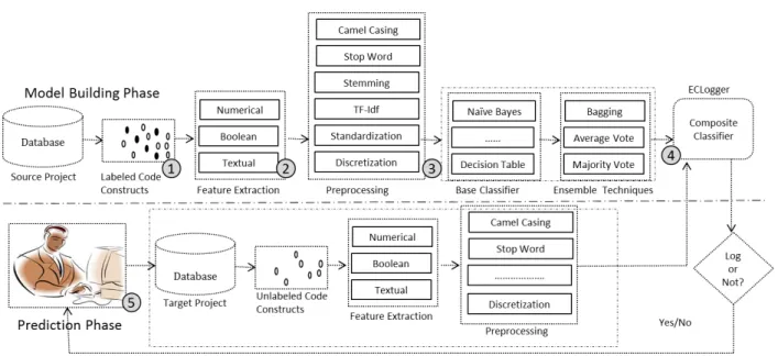
Figure 1. Overview of the proposed ECLogger framework
as logged, it is predicted as logged; otherwise, it is predicted as non-logged.
4. ECLogger model
Figure 1 presents the framework of ECLogger. It consists of two main phases: model building and prediction (refer to Figure 1). In the model building phase, a cross-project logging predic-tion model is build from the labelled instances of the source project. There are 4 main steps in the model building phase: training instance collection (Step 1), feature extraction (Step 2), pre-processing (Step 3), and ECLogger model building (Step 4) (refer to Step 1 to Step 4 in Figure 1). In the prediction phase, the label (logged or non-logged) of the new instance in the target project is predicted (refer to Step 5 in Figure 1). Algorithm 1 shows the sequence of operations performed by the ECLogger model and the details of the experimental setup (re-fer to Table 1 for details regarding the notations used). In Algorithm 1, lines 2–6, 11, 15 and 21–22 correspond to the experimental setup, whereas, other lines correspond to the steps of the ECLog-ger model. The lines 24–26 and 28–32 defines the functions that are part of the experimental setup. The lines 34–39 and 41–49 define the
func-tions that are part of the ECLogger model. The following are the main steps of the ECLogger model:
4.1. Phase 1: (model building)
Training instance collection (step 1): The experimental dataset consists of three projects: Tomcat, CloudStack and Hadoop. One project is considered as the source project (SP), i.e. train-ing project, and the other two projects as the target project (T P), i.e. testing project, a sin-gle project at a particular instance. Using this, 6 source and target project pairs are created (lines 7–10 in Algorithm 1). EClogger extracts all logged and non-logged catch-blocks (CBSP) from the source project for training.
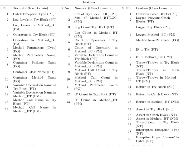
Feature extraction (step 2): ECLogger extracts all the features from the source catch-blocks (CBSP) for training as initial source features (F VISP) (refer to function ExtractFeatures(), i.e. lines 34–39 in Algo-rithm 1). All 46 features proposed by Lal et al. [10] are used for catch-block logging predic-tion on Java projects (refer to Table 2). These features are selected because they have shown promising results for within-project catch-block logging prediction [10]. Lal et al. [10] described three properties for the features, i.e. domain, type
Algorithm 1. ECLogger Algorithm 1: procedureECLogger 2: P ={PT,PC,PH} 3: A={AADA,AADT,ABN,ADT,AJ48,ALR,ANB,ARF,ARBN} 4: EA={EABA,EAMV,EAAV} 5: M=10 6: CS={3,4,5,6,7,8,9} 7: forallS∈P do 8: forallT ∈P do 9: if S≠T then 10: SP=S,T P =T 11: CBSP =ReadCompleteData(SP) 12: F VISP=ExtractFeatures(CBSP) 13: F VFSP=Preprocess(F VISP)
14: ECLoggerModel[]=BuildModel(F V F SP,A,EA,CS) 15: CBT P[M]=ReadBalanceData(T P) 16: fori=1 to size(ECLoggerModel)do 17: forj=1 toM do 18: F VIT P =ExtractFeatures(CB)T P[j]) 19: F VFT P =Preprocess(F VIT P)
20: PD[i][j]=ApplyModel(F VFT P,ECLoggerModels[j]) 21: AR[i]= M ∑ j=1 PD[i][j] M
22: BMSP→T P =FindBestModel(AR,ECLoggerModels) 23: procedureReadCompleteData(P) 24: CB=ReadCatchBlocks(P) 25: returnCB 26: procedureReadBalanceData(P, M) 27: CB=ReadCatchBlocks(P) 28: CB̂ =Randomize(CB) 29: BS[]=Generate_M_BalanceSamples(CB̂) 30: returnBS 31: procedureExtractFeatures(CB) 32: TF V=getTextualFeatures(CB) 33: NF V =getNumericFeatures(CB) 34: BF V =getBooleanFeatures(CB) 35: F V ={TF V,NF V,BF V} 36: returnF V 37: procedurePreprocess(F V)
38: TF Vˆ =TF_IDFConversion(Stemming(StopWordRemoval(CamelCaseSeparation(TF V)))) 39: if It is Test Datathen
40: TF Ṽ=FilterFeatureNotTrainData(TF V̂) 41: else
42: TF Ṽ= T̂F V
43: F VF =Discretization(Standardization(Combine(TF Ṽ,BF V,NF V))) 44: returnF VF
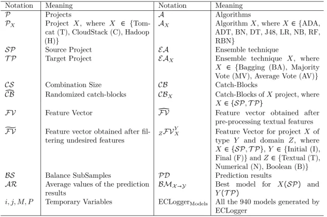
Table 1. Notations used in the ECLogger Algorithm (i.e. Algorithm 1)
Notation Meaning Notation Meaning
P Projects A Algorithms
PX Project X, where X ∈ {Tom-cat (T), CloudStack (C), Hadoop (H)}
AX AlgorithmX, whereX ∈{ADA, ADT, BN, DT, J48, LR, NB, RF, RBN}
SP Source Project EA Ensemble technique
T P Target Project EAX Ensemble technique X, where
X ∈ {Bagging (BA), Majority Vote (MV), Average Vote (AV)}
CS Combination Size CB Catch-Blocks ̂
CB Randomized catch-blocks CBX Catch-Blocks ofX project, where
X ∈{SP,T P}
F V Feature Vector ̂F V Feature vector obtained after pre-processing textual features ̃
F V Feature vector obtained after fil-tering undesired features
ZF V Y
X Feature Vector for project X of type Y and domain Z, where
X ∈{SP,T P},Y ∈{Initial (I), Final (F)} andZ ∈{Textual (T), Numerical (N), Boolean (B)}
BS Balance SubSamples PD Prediction results
AR Average values of the prediction results
BMX→Y Best model for X(SP) and
Y(T P)
i, j, M, P Temporary Variables ECLoggerModels All the 940 models generated by
ECLogger
and class. Domain indicates from which part of the source code a particular feature is extracted. Type indicates whether a features is numeric, boolean, or textual.Classindicates whether a fea-ture belongs to a positive class or a negative class. In Table 2, the features are categorized based on their type. ECLogger extracts all three types of features for model building. For example, the size a try-block (refer to numeric feature 1 in Table 2) is a numeric feature that computes the SLOC of try-blocks associated with logged and non-logged catch-blocks and that belong to the try/catch domain. All the features with their respective properties are listed in Table 2. Pre-processing (step 3): Six pre-processing steps are applied to clean the initial source fea-tures (F VISP). First the textual features are celaned. All the terms concatenated using the camel-casing in the textual features (i.e. ‘getTar-get’ is converted to ‘‘getTar-get’, ‘tar‘getTar-get’) are separated. Subsequently, all the English stop words from the textual features are removed. The used stop word list was provided by the Python nltk tool [60]. Then stemming is applied (the Porter stemming
algorithm by the nltk tool [60]) on all the textual features and converted all the textual features to their tf-idf transformation to create the tex-tual feature vector. The textex-tual feature vector is then combined with numerical and boolean feature vectors. To address the problem of data heterogeneity in the source and target projects, data standardization was performed, i.e. feature values were converted to a z-distribution. Nam et al. [14] demonstrated the usefulness of data normalization for the cross-project defect pre-diction problem. Finally, all the features were discretized, as some algorithms, such as Naïve Bayes, work only with discretized data. Using this, the final feature vector (F VFSP) for train-ing the model (refer to function Preprocess() is obtained, i.e. lines 41–49 in Algorithm 1). ECLogger model building (step 4): ECLog-ger models were built using 9 base classi-fiers (ADA, ADT, BN, DT, J48, LR, NB, RF, and RBF) and three ensemble techniques (bagging, average voting and maximum vot-ing). Bagging was applied on 8 of the 9 base classifiers. We create 8 ECLoggerBagging
mod-Table 2. Features used for cross-project catch-block logging prediction taken from previously published work by Lal et al. [10]. PT: class = positive, domain = try/catch; PM: class = positive, domain = method_bt; PO: class = positive, domain = other; NT: class = negative, domain = try/catch; and NM: class = negative,
domain = method_bt
Features
S. No. Textual (Class Domain) S. No. Numeric (Class Domain) S. No. Boolean (Class Domain) 1 Catch Exception Type (PT) 1 Size of Try Block [LOC] (PT) 1 Previous Catch Blocks (PT) 2 Log Levels in Try Block (PT) 2 (PM)Size of Method_BT[LOC] 2 Logged Previous CatchBlocks (PT) 3 (PM)Log Levels in Method_BT 3 Log Count Try Block (PT) 3 Logged Try Block (PT) 4 Operators in Try Block (PT) 4 (PM)Log Count in Method_BT 4 Logged Method_BT (PM) 5 (PM)Operators in Method_BT 5 Count of Operators in TryBlock (PT) 5 Method have Parameter (PO) 6 (PO)Method Parameters (Type) 6 CountMethod_BT (PM)of Operators in 6 IF in Try (PT)
7 (PO)Method Parameters (Name) 7 Variable Declaration Count inTry Block (PT) 7 IF in Method_BT (PM) 8 (PO)Container Package Name 8 Variable Declaration Count inMethod_BT (PM) 8 (NT)Throw/Throws in Try Block 9 Container Class Name (PO) 9 Method Call Count in TryBlock (PT) 9 Throw/ThrowsBlock (NT) in Catch 10 (PO)Container Method Name 10 MethodMethod_BT (PM)Call Count in 10 Throw/Throws in Method_-BT (NM) 11 Variable Declaration Name inTry Block (PT) 11 (PO)Method Parameter Count 11 Return in Try Block (NT) 12 Variable Declaration Name inMethod_BT (PM) 12 IF Count in Try Block (PT) 12 Return in Catch Block (NT) 13 Method Call Name in TryBlock (PT) 13 (PM)IF Count in Method_BT 13 Return in Method_BT (NM) 14 MethodMethod_BT (PM)Call Name in 14 Assert in Try Block (NT)
15 Assert in Catch Block (NT) 16 Assert in Method_BT (NM) 17 (NT)Thread.Sleep in Try Block 18 (NT)Interrupted Exception Type 19 Exception Object "Ignore" inCatch (NT) Total Features = 46 (Textual (14) + Numeric (13) + Boolean (19))
els, i.e. BaggingADA, BaggingADT, BaggingBN, BaggingJ48, BaggingLR, BaggingNB, BaggingRF and BaggingRBF. BaggingADA is an ECLogger model that is generated by applying bagging on the ADA classifier. Bagging was not applied on the decision table (DT) classifier because of its high time complexity.
The number of created ECLogger average vote models was 466. One can take an average vote of n classifiers to perform a logging pre-diction on a new code construct. For example, ADA-ADT-BN is one possible combination of 3 classifiers which can be chosen to take an average vote. In this case,the best value of n (i.e. number of classifiers to take) is not known
similarly to the information which classifiers are the most suitable for cross-project logging pre-diction. Hence, all possible combinations of base classifiers are created for n = {3,4,5,6,7,8,9}. Using this strategy, 466 ECLoggerAverageVote mod-els are created. Similarly to ECLoggerAverageVote, 466 ECLoggerMajorityVotemodels are created. 940 distinct ECLogger models (ECLoggerModels[]) are created for cross-project logging prediction (line 14 in Algorithm 1).
4.2. Phase 2: (prediction)
Prediction (step 5): In the prediction phase, ECLoggerModelsare used to predict the label of
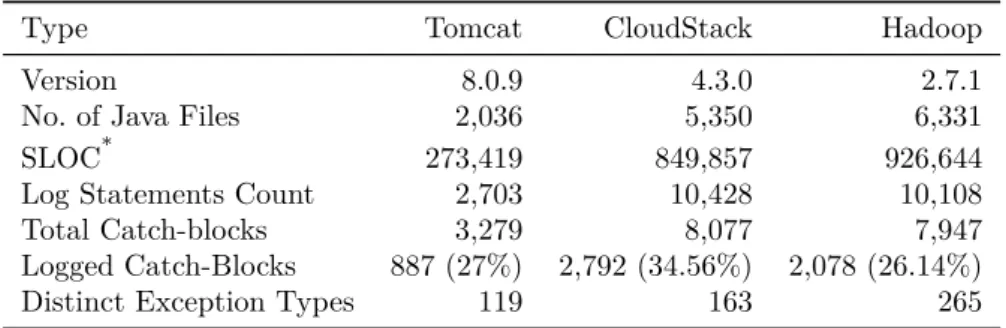
Table 3. Experimental dataset details
Type Tomcat CloudStack Hadoop
Version 8.0.9 4.3.0 2.7.1
No. of Java Files 2,036 5,350 6,331 SLOC* 273,419 849,857 926,644 Log Statements Count 2,703 10,428 10,108 Total Catch-blocks 3,279 8,077 7,947 Logged Catch-Blocks 887 (27%) 2,792 (34.56%) 2,078 (26.14%) Distinct Exception Types 119 163 265
*
Computed using: http://www.locmetrics.com/.
a new code construct in the target project. All the catch-blocks are extracted from the target project and all the pre-processing techniques de-scribed in Step 3 are applied. In addition to these pre-processing steps, one additional filter-ing step is applied in the prediction phase. In cross-project prediction, there is a possibility that some features that are present in the source project (F VFSP) may not be available in the tar-get project (because of a vocabulary mismatch). Hence, in the target project, the features that are absent in the source project (line 44 in Al-gorithm 1) are eliminated. Using this, the final feature vector (F VFT P) for the target project in-stance is created. Then all the ECLogger mod-els to predict the labmod-els of target project in-stances are applied. For each source and tar-get project pair, the ECLoggerModel(BMSP→T P)
that provides the best performance (mea-sured in terms of average LF) is then identified.
5. Experimental details
In this section, we present details related to the experiments performed in this work. We present details regarding dataset selection, dataset prepa-ration, experimental environment, design of the experiment, and evaluation metrics.
5.1. Experimental dataset selection To facilitate the replication of this study, all of our experiments were conducted on open-source
Java projects from the Apache Software Founda-tion (ASF1). The ASF consists of a large number of actively maintained and widely used projects. Hence, it is believed that the projects from the ASF consist of good logging and are suitable for our study. We select projects from the ASF that match the following criteria:
1. Number of files:The selected projects have have at least 1000 files so that statistically significant conclusions can be drawn.
2. Number of catch-blocks: The selected projects have at least 1000 catch-blocks so that statistically significant conclusions can be drawn.
3. Programing language: The selected projects are written in the Java programing language. Java projects are selected because Java is one of the most widely used program-ming languages [61].
Three projects matching the above criteria are selected: Tomcat [62], CloudStack [63], and Hadoop [64] (see Tab. 3). All of these projects are widely used and have previously been used in logging studies [10, 13, 23, 65].
5.2. Experimental dataset preparation The catch-blocks (see Tab. 3) are extracted from the three projects, i.e. Tomcat, CloudStack and Hadoop. A catch-block is marked as logged (+ve class) if it consists of at least one log statement; otherwise, it is marked as non-logged (–ve class). Numerous variations are observed in the usage format of log statements in the three projects. Hence, 26 regular expressionsare created to
ex-1
tract all types of logging statements present in the catch-blocks.
5.3. Experimental environment
The WEKA [48] implementation is used for all the classifiers. The default parameters are used for all the classifiers. All of our experiments are run on Windows Server 2012, with 64 GB RAM, 64-Bit operating system, and an Intel® Xeon® CPU E5-2640 0, 2.50 GHz processor (2 proces-sors), 6 cores per processor.
5.4. Design of the experiment
Two types of experiments were performed: within-project and cross-project catch-block log-ging prediction. The following presents the ex-perimental design for both types of predictions: Within-project prediction: To compute the within-project logging prediction, 10 equal-sized balanced datasets for each project were created, namely,Tomcat, CloudStack, and Hadoop. Be-cause the number of –ve class (non-logged) in-stances is higher than that of +ve class (logged) instances, the subsampling of –ve class instances were performed to make the dataset balanced. In this way, 10 random samples (with replacement) were created from the database. The majority class (–ve class) subsampling technique was used in previous studies to balance the dataset [10,66]. On the balanced dataset, a 70/30 training-testing split is used and the average results over the 10 datasets are reported.
Cross-project prediction: To conduct the cross-project logging prediction experiment, training and testing datasets are created. All the catch-blocks of the source projects are used for training. For the purpose of testing, 10 balanced subsamples of catch-blocks of the target projects are created, i.e. the same as the ones created for the within-project logging prediction. Using this, 10 datasets that have the same training dataset and different test-ing datasets are created. The results are com-puted for each of the 10 datasets and report the average results over 10 datasets. Train-ing and testTrain-ing datasets are created (it is pre-ferred solution to using 10-fold cross validation)
to compare the effectiveness of multiple mod-els. This is because in the cross-project predic-tion the model is trained on the source project and tested on the traget project. Furthermore, separation of training and testing data using 10-fold cross-validation is challenging in this con-text.
5.5. Evaluation metrics
In this subsection, the performance metrics used to evaluate the effectiveness of the prediction model is described. Five metrics were used in the evaluation process: precision, recall, accu-racy, F-measure, and area under the ROC curve. All of these are widely used metrics and were previously used in logging prediction and defect prediction studies [8,10,11,30,67]. There are four possible outcomes while predicting the logging of a code construct:
1. Predicting logged code construct as logged, l→l(true positive).
2. Predicting logged code construct as non-logged, l→n(false negative).
3. Predicting non-logged code constructs as non-logged, n→n(true negative).
4. Predicting non-logged code constructs as logged, n→l (false positive).
After constructing the classifier on the train-ing set, its performance on the test set can be evalauted. The total number of logged code constructs predicted as logged (Cl→l), logged
code constructs falsely predicted as non-logged (Cl→n), non-logged code constructs predicted as
non-logged (Cn→n), and non-logged code
con-structs predicted and logged (Cn→l) are
com-puted. Using these 4 values, the following metrics are defined:
Logged Precision: It shows the percentage of code constructs that are correctly labelled as logged among those labelled as logged.
Logged Precision (LP)=
Cl→l
Cl→l+Cn→l
×100 (2) Logged Recall: It shows the proportion of logged code constructs that are correctly labelled as logged.
Logged Recall (LR)= Cl→l
Cl→l+Cl→n
×100 (3) Logged F-measure: It is a metric that com-bines logged precision and recall. Precision and recall metrics have a trade-off. One can increase precision (recall) by decreasing recall (precision) [39, 68]. Hence, it is difficult to evaluate the per-formance of different prediction algorithms us-ing only one of the precision or recall metrics. F-measure computes the weighted harmonic mean of precision and recall and is hence useful in over-coming the precision and recall trade-off. It has been widely used in the software engineering lit-erature for performance evaluation [42, 69, 70]. Equation (4) shows the formula to compute the LF metric. In this equation, β is a weighting parameter, where the value of β less than one emphasizes precision and greater than one empha-sizes recall. In this paper,β=1, which gives equal weightage to both precision and recall, is used.
Logged F-measure(LF)=
(β2+1)×LP ×LR
β2×LP +LR ×100 (4) Accuracy: It computes the percentage of code constructs that are correctly labelled as logged or non-logged to the total number of code con-structs. It is also a widely used metric for evalu-ating the performance of prediction models. Ac-curacy is found to be a biased metric in the case of imbalanced datasets. However, in this work, testing was performed only on balanced datasets.
Accuracy(ACC)=
Cl→l+Cn→n
Cl→l+Cl→n+Cn→n+Cn→l ×
100 (5) Area under the ROC curve (RA): It mea-sures the likelihood that a logged code construct is given a high likelihood score compared to a non-logged code construct. RA can take any value in the range 0 to 1. In general, higherRA values are considered better, i.e. an RA value of 1 is the best.
6. Experimental results
In this section, the eight identified research ques-tions (RQs) are addressed. The following subsec-tions elaborate the motivation, approach, and results for each of the identified RQs.
6.1. Research questions
Eight RQs are categorized in two dimensions. RQ1–RQ4 investigate the performance of single classifiers for cross-project catch-block logging prediction, whereas RQ5–RQ8 examine the per-formance of the ECLogger models.
Research Objective 1 (RO1): Perfor-mance of the single classifier for cross-project catch-block logging prediction
– RQ1: How is the performance of within-pro-ject different from cross-prowithin-pro-ject catch-block logging prediction?
– RQ2: Which is better, the single-project or multi-project training model for cross-project catch-block logging prediction?
– RQ3: Are different classifiers complimentary to each other when applied to cross-project catch-block logging prediction?
– RQ4: Are the algorithms that perform best for within-project and cross-project catch-block logging predictions identical? Research Objective 2 (RO2) : Performance of ensemble-based classifiers, i.e. ECLogger mod-els, for cross-project catch-block logging predic-tion.
– RQ5: What is the performance of ECLoggerBaggingfor cross-project catch-block logging prediction?
– RQ6: What is the performance of ECLoggerAverageVote for cross-project catch-block logging prediction?
– RQ7: What is the performance of ECLoggerMajorityVote for cross-project catch-block logging prediction?
– RQ8:What is the average performance of the baseline classifier and ECLoggerModels over all the source and target project pairs?
TC->TC CS->CS HD->HD CS->TC HD->TC TC->CS HD->CS TC->HD CS->HD Source Project -> Target Project
0 20 40 60 80 100 Average LF (%)
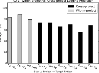
RQ 1: Within-project vs. Cross-project Logging Prediction Cross-project Within-project
Figure 2. The highest averageLF of within-project and cross-project logging predictions. CS: CloudStack, TC: Tomcat, and HD: Hadoop
Table 4. Within-project catch-block logging prediction results (using a single classifier). ML ALGO: Machine Learning Algorithm
Project: Tomcat
Total Instances: 1,774, Features: 1,522
ML ALGO Avg.LP (%) Avg.LR(%) Avg.LF (%) Avg.ACC(%) Avg.RA(%) ADA 75.13±4.76 78.55±11.82 75.97±2.84 76.56±1.13 86.6±0.97 ADT 73.82±3.72 88.59±8.86 80.08±2.05 79.06±1 88.16±0.99 BN 74.79±1.07 81.92±0.75 78.18±0.55 78.08±0.7 87.45±0.76 DT 76.19±2.2 72.12±5.82 73.98±3.16 75.81±2.39 84.12±1.76 J48 80.45±1.7 83.45±2.5 81.92±1.95 82.35±1.81 86.17±2.06 LR 79.98±2.12 86.35±1.2 83.03±1.36 83.06±1.53 91.64±0.94 NB 74.56±1.12 81.76±0.77 77.99±0.61 77.88±0.76 87.25±0.74 RF 80.93±2.77 82.71±1.96 81.79±2 82.33±2.07 90.37±1.07 RBF 57.98±0.98 93.14±3.63 71.42±0.92 64.3±1.08 75.19±0.87 Project: CloudStack
Total Instances: 5,584, Features: 1,332
ML ALGO Avg.LP (%) Avg.LR(%) Avg.LF (%) Avg.ACC(%) Avg.RA(%) ADA 72.28±3.94 93.34±7.06 81.13±0.4 78±1.23 85.9±1.31 ADT 79.74±1.99 92.42±3.01 85.54±0.39 84.16±0.43 92.11±0.48 BN 73.6±0.45 94.89±0.45 82.9±0.3 80.14±0.39 89.34±0.4 DT 83.18±1.27 85.34±2.49 84.23±1.63 83.8±1.56 91.54±1.17 J48 88.43±1.25 88.12±2 88.25±0.74 88.1±0.66 91.69±0.58 LR 87.61±0.41 87.28±0.83 87.45±0.52 87.28±0.49 94.16±0.53 NB 73.54±0.49 94.76±0.49 82.81±0.32 80.04±0.43 89.2±0.39 RF 86.21±0.96 90.86±0.99 88.47±0.85 87.98±0.88 94.93±0.28 RBF 55.02±1.52 100±0 70.97±1.28 58.44±2.64 57.79±2.68
Project: Hadoop, Type: Catch-Block Total Instances: 4,156, Features: 1,322
ML ALGO Avg.LP (%) Avg.LR(%) Avg.LF (%) Avg.ACC(%) Avg.RA(%) ADA 73.74±0.89 74.74±2 74.22±1.13 74.53±0.92 81.06±0.42 ADT 75.28±1.93 78.64±1.88 76.89±0.81 76.79±1 83.17±0.25 BN 74.11±1.12 65.18±0.89 69.35±0.72 71.72±0.72 81.06±0.63 DT 76.76±1.66 76.13±2.56 76.4±1.12 76.93±0.96 83.27±0.7 J48 77.89±1.89 79.74±1.59 78.78±0.93 78.91±1.1 81.57±1.21 LR 78.74±1.08 80±0.94 79.36±0.62 79.57±0.68 87.25±0.5 NB 74.08±1.09 65.13±0.84 69.31±0.69 71.69±0.7 80.97±0.63 RF 77.9±0.91 77.75±1.27 77.82±0.94 78.25±0.88 86.28±0.65 RBF 57.07±0.81 76.68±4.87 65.39±2.27 60.27±1.33 59.32±1.64
6.2. RO1: Performance of the single classifier for cross-project catch-block logging prediction
In this subsection four RQs (RQ1–RQ4), which investigate the performance of single classifiers, are answered. The questions related to the vari-ation in performance of a single classifier for within-project and cross-project logging predic-tions using multiple evaluation metrics, using both single-project and multi-project training models are answered.
6.2.1. RQ1: How is the performance of
within-project different from cross-project catch-block logging prediction
Motivation: IIn RQ1, the effectiveness of within-project and cross-project logging predic-tion models (using a single classifier) are com-pared. Cross-project logging prediction is chal-lenging, and hence, it is important to identify the performance variation of the cross-project logging prediction model compared to that of the within-project logging prediction model. The results from this investigation can provide im-portant insights and motivation for constructing the cross-project logging prediction model. Approach: To answer RQ1, the performances of single classifiers for within-project and cross-project logging prediction are compared. The average LF is used to compare the perfor-mances of different classifiers.
Results: Table 4 presents the detailed results of within-project catch-block logging prediction for all three projects. Our experimental results show that the RF and LR models outperform other al-gorithms in terms of averageLF. The highest av-erageLF of 83.03%, 88.47%, and 79.36% for the within-project catch-block logging prediction was achieved on the Tomcat, CloudStack and Hadoop projects, respectively. Figure 2 shows the highest averageLF values from the within-project and cross-project experiments. Figure 2 shows that the highest average LF for all six cross-project results is lower than all three within-project re-sults. Table 5, Table 6 and Table 7 show the detailed cross-project logging prediction results
(using a single classifier). These experimental results show that for the cross-project logging prediction, the highest average LF of 73.66%, 70.42% and 68.62% was achieved for the Tomcat, CloudStack and Hadoop projects, respectively. A 6.37% to 18.05% decrease was observed in the classification performance for cross-project logging prediction compared to within-project logging prediction. The performance of the RBF classifier is the worst for cross-project logging prediction. For all six pairs of source and target project pairs, RBF provides an averageLF of 0% and averageACC of 50%, i.e. predicting all the code constructs as non-logged (refer to Table 5, Table 6, and Table 7).
A 6.37% to 18.05% decrease was observed in the average LF for cross-project logging pre-diction compared to within-project logging prediction.
6.2.2. RQ2: Which is better, the single-project or multi-project training model for cross-project catch-block logging prediction?
Motivation: In RQ2, the objective is to exam-ine the effectiveness of multi-project training for cross-project logging prediction. Thus it is necessary to ascertain whether information fu-sion enhances the accuracy of the cross-project logging prediction. Training a predictive model from multiple projects is one type of informa-tion fusion-based approach and was shown to enhance accuracy because it involves combining information from multiple sources. Few stud-ies in the past used multi-project training for cross-project defect prediction [30, 71]. However, for cross-project logging prediction, this has yet to be explored. The answer to this RQ can provide important insights about selecting the single-project or multi-project cross-project log-ging prediction model.
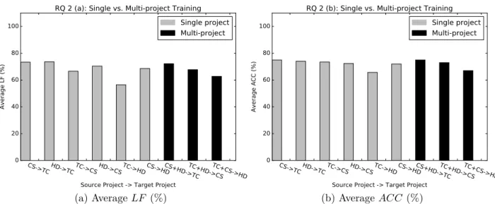
Approach: Approach: To answer RQ2, 9 pairs of source and target projects are created, i.e. 6 pairs consisting of one source project and 3 pairs consisting of two source projects. Results: Figure 3 presents the histogram of the average LF and average ACC
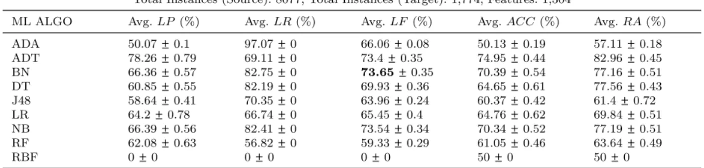
val-Table 5. Cross-project catch-block logging prediction results (using a single classifier) for Tomcat (target project). ML ALGO: Machine Learning Algorithm
Project: CloudStack→Tomcat
Total Instances (Source): 8077, Total Instances (Target): 1,774, Features: 1,304
ML ALGO Avg.LP (%) Avg.LR(%) Avg.LF (%) Avg.ACC(%) Avg.RA(%) ADA 50.07±0.1 97.07±0 66.06±0.08 50.13±0.19 57.11±0.18 ADT 78.26±0.79 69.11±0 73.4±0.35 74.95±0.44 82.96±0.45 BN 66.36±0.57 82.75±0 73.65±0.35 70.39±0.54 77.16±0.51 DT 60.85±0.55 82.19±0 69.93±0.36 64.65±0.61 77.56±0.43 J48 58.64±0.41 70.35±0 63.96±0.24 60.37±0.42 61.4±0.72 LR 64.2±0.78 66.74±0 65.45±0.4 64.76±0.62 69.84±0.51 NB 66.39±0.56 82.41±0 73.54±0.34 70.34±0.52 77.19±0.51 RF 62.08±0.63 56.82±0 59.33±0.29 61.05±0.46 63.64±0.49 RBF 0±0 0±0 0±0 50±0 50±0
Project: Hadoop→Tomcat
Instances (Source): 7,947, Instances (Target): 1,774, Features: 1,313
ML ALGO Avg.LP (%) Avg.LR(%) Avg.LF (%) Avg.ACC(%) Avg.RA(%) ADA 85.5±0.88 49.15±0 62.42±0.24 70.41±0.3 79.45±0.32 ADT 79.37±0.95 55.36±0 65.22±0.32 70.48±0.42 77.96±0.44 BN 74.74±0.67 72.49±0 73.6±0.33 73.99±0.44 80.17±0.47 DT 84.98±0.94 52.2±0 64.67±0.27 71.48±0.34 77.17±0.33 J48 65.82±0.65 65.95±0 65.88±0.33 65.85±0.5 66.8±0.66 LR 76.52±0.72 54.57±0 63.7±0.25 68.91±0.34 76.99±0.43 NB 74.76±0.64 72.6±0 73.66±0.31 74.04±0.41 80.19±0.47 RF 67.91±1.06 39.46±0 49.91±0.29 60.4±0.46 67.2±0.52 RBF 0±0 0±0 0±0 50±0 52.77±0.93
Table 6. Cross-project catch-block logging prediction results (using a single classifier) for CloudStack (target project). ML ALGO: Machine Learning Algorithm
Project: Tomcat→CloudStack
Total Instances (Source): 3,279, Total Instances (Target): 5,584, Features:1,425
ML ALGO Avg.LP (%) Avg.LR(%) Avg.LF (%) Avg.ACC(%) Avg.RA(%) ADA 87.84±0.49 53.19±0 66.26±0.14 72.91±0.17 81.45±0.22 ADT 90.12±0.41 52.79±0 66.58±0.11 73.5±0.13 80.95±0.13 BN 63.46±0.39 69.41±0 66.3±0.21 64.72±0.34 71.7±0.38 DT 72.75±0.33 45.38±0 55.89±0.1 64.19±0.14 74.41±0.16 J48 66.36±0.44 56.91±0 61.28±0.19 64.03±0.28 63.32±0.34 LR 80.48±0.56 48.14±0 60.24±0.16 68.23±0.21 74.94±0.14 NB 63.36±0.39 69.23±0 66.16±0.21 64.59±0.34 71.7±0.38 RF 80.84±0.38 37.29±0 51.03±0.08 64.22±0.11 75.45±0.18 RBF 0±0 0±0 0±0 50±0 63.11±0.44
Project: Hadoop→CloudStack
Instances (Source): 7,947, Instances (Target): 5,584, Features: 1,313
ML ALGO Avg.LP (%) Avg.LR(%) Avg.LF (%) Avg.ACC(%) Avg.RA(%) ADA 83.44±0.59 49.61±0 62.22±0.16 69.88±0.21 79.79±0.25 ADT 88.64±0.36 51.33±0 65.01±0.1 72.37±0.12 81.86±0.16 BN 64.25±0.29 77.87±0 70.41±0.17 67.27±0.27 76.79±0.29 DT 84.71±0.5 45.95±0 59.58±0.12 68.83±0.16 74.65±0.2 J48 64.58±0.38 58.45±0 61.37±0.17 63.2±0.27 65.21±0.28 LR 83.19±0.5 55.73±0 66.75±0.16 72.23±0.2 79.03±0.2 NB 64.25±0.29 77.9±0 70.42±0.17 67.27±0.27 76.8±0.29 RF 83.91±0.57 36.1±0 50.48±0.1 64.59±0.15 73.11±0.25 RBF 0±0 0±0 0±0 50±0 57.72±0.42
Table 7. Cross-project logging prediction results (using a single classifier) for Hadoop (target project). ML ALGO: Machine Learning Algorithm
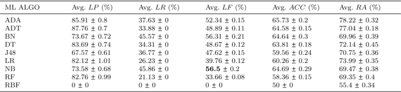
Project: Tomcat→Hadoop
Total Instances (Source): 3,279, total instances (target): 4,156, features: 1,425
ML ALGO Avg.LP (%) Avg.LR(%) Avg.LF(%) Avg.ACC(%) Avg.RA(%) ADA 85.91±0.8 37.63±0 52.34±0.15 65.73±0.2 78.22±0.32 ADT 87.76±0.7 33.88±0 48.89±0.11 64.58±0.15 77.04±0.18 BN 73.67±0.72 45.57±0 56.31±0.21 64.64±0.3 69.96±0.39 DT 83.69±0.74 34.31±0 48.67±0.12 63.81±0.18 72.14±0.45 J48 67.57±0.61 36.77±0 47.62±0.15 59.56±0.24 70.75±0.36 LR 82.12±1.01 26.23±0 39.76±0.12 60.26±0.2 73.99±0.35 NB 73.58±0.68 45.86±0 56.5±0.2 64.69±0.29 69.47±0.38 RF 82.76±0.99 21.13±0 33.66±0.08 58.36±0.15 69.35±0.4 RBF 0±0 0±0 0±0 50±0 55.4±0.34
Project: CloudStack→Hadoop
Instances (source): 8,077, instances (target): 4,156, features: 1,304
ML ALGO Avg.LP (%) Avg.LR(%) Avg.LF(%) Avg.ACC(%) Avg.RA(%) ADA 50.29±0.06 98.12±0 66.5±0.05 50.57±0.12 54.24±0.1 ADT 79.55±0.56 52.12±0 62.97±0.18 69.36±0.23 76.51±0.27 BN 57.26±0.3 79.74±0 66.65±0.2 60.11±0.36 68.2±0.39 DT 77.99±0.36 61.26±0 68.62±0.14 71.99±0.18 76.31±0.14 J48 73.4±0.65 58.13±0 64.88±0.25 68.53±0.35 69.99±0.45 LR 72.76±0.95 55.58±0 63.02±0.36 67.38±0.5 71.83±0.61 NB 57.31±0.28 79.69±0 66.67±0.19 60.16±0.34 68.16±0.39 RF 66.35±0.77 46.92±0 54.97±0.26 61.56±0.41 67.32±0.41 RBF 0±0 0±0 0±0 50±0 50±0
ues of multi-project cross-project catch-block logging prediction. Figure 3a reveals that there is no dominant approach between sgle-project and multi-project. In certain in-stances, multi-project training increased the prediction performance, and in other cases it has decreased the prediction performance. For example, in the CloudStack project when single source-project training is used, the highest average LF of 66.5% (source project Tomcat) and 70.42% (source project Hadoop) are achived (refer to Table 6). In contrast, when multi-project training is used and both Tomcat and Hadoop are ap-plied to build the model, the highest av-erage LF of 67.74% is achieved. Hence, multi-project training causes a 1.24% decrease and a 2.68% increase in the prediction per-formance of single-project training when Tom-cat and Hadoop are used, respectively. A sim-ilar result is observed for the ACC metric (refer to Figure 3b).
There is no dominant approach among the single-project and multi-project cross-project catch-block prediction models.
6.2.3. RQ3: Are different classifiers complimentary to each other when applied to cross-project catch-block logging prediction?
Motivation: In RQ3, the objective is to exam-ine the performance of individual classifiers on multiple evaluation metrics. The evaluation of a predictive model or a classifier can be per-formed using several metrics or measures, and the selected set of metrics depends on the classi-fication task and problem. The Authors believe that the answer to this research question will provide important insights about combining dif-ferent classifiers (using an ensemble of classifiers) for improving the cross-project logging prediction performance.
Approach: Individual classifiers are compared on 5 evaluation metrics, namely, average LP, average LR, averageLF, averageACC, and av-erage RA, to identify whether a single classifier dominates and provides the highest values over all the evaluation metrics.
Results: The results indicate that different classifiers are complementary to each other. For
CS->TC HD->TC TC->CS HD->CS TC->HD CS->HDCS+HD->TCTC+HD->CSTC+CS->HD Source Project -> Target Project
0 20 40 60 80 100 Average LF (%)
RQ 2 (a): Single vs. Multi-project Training Single project Multi-project
(a) AverageLF (%)
CS->TC HD->TC TC->CS HD->CS TC->HD CS->HDCS+HD->TCTC+HD->CSTC+CS->HD Source Project -> Target Project
0 20 40 60 80 100 Average ACC (%)
RQ 2 (b): Single vs. Multi-project Training Single project Multi-project
(b) AverageACC (%)
Figure 3. The Highest AverageLF of Single-project and Multi-project Training Logging Prediction Models. CS: CloudStack, TC: Tomcat, and HD: Hadoop
AVG. LP AVG. LR AVG. LF AVG. ACC AVG. RA Metric 0 20 40 60 80 100 Values(%)
RQ 3(a): Single Classifier Performance (CS->TC) ADA ADT BN
(a) Classifier performance for the CS→TC project pair
AVG. LP AVG. LR AVG. LF AVG. ACC AVG. RA Metric 0 20 40 60 80 100 Values(%)
RQ 3(b): Single Classifier Performance (HD->CS) NB ADT
(b) Classifier performance for the HD→CS project pair
Figure 4. The Results (averageLP,LR,LF,ACC andRA) of Selected Single Classifiers. CS: CloudStack, TC: Tomcat, and HD: Hadoop
example, consider the results obtained on the following source and target project pair:
CloudStack (source)→Tomcat (target):
Figure 4a presents the histogram of all five metrics (LP, LR, LF, ACC and RA) for the CloudStack→Tomcat project pair for the ADA,
ADT and NB classifiers. ADA, ADT and NB are selected because these three classifiers pro-vide the best results for cross-project catch-block logging prediction on the CloudStack→Tomcat
project pair. Figure 4a shows that the ADT model provides the highest average LP, ACC
andRA values, whereas ADA and BN provide the highest average LR and LF, respectively (refer to Table 5 for detailed results).
Hadoop (source)→CloudStack (target):
Similarly to Figure 4a, Figure 4b presents the histogram of all 5 metrics for the Hadoop→CloudStack project pair for the ADT
and NB classifiers. Figure 4b shows that NB provides the highest average LR and LF val-ues, whereas ADT provides the highest average LP,ACC, and RAvalues (refer to Table 6 for detailed results).
The above two examples indicate that differ-ent classifiers provide complemdiffer-entary informa-tion for cross-project catch-block logging predic-tion and, hence, their ensemble can be benefi-cial for improving the results of the prediction model [72].
The results indicate that the different clas-sifiers are complementary to each other for cross-project catch-block logging prediction. 6.2.4. RQ4: Are the algorithms that perform
best for within-project and cross-project catch-block logging predictions identical? Motivation: In a related work, Zhu et al. [11] used the same algorithm (J48) for both within-project and cross-project logging pre-dictions. However, there is a possibility that the same algorithm is not suitable for both within-project and cross-project logging predic-tions. In RQ4, the performances of different clas-sifiers for within-project and cross-project logging predictions are compared. The Authors believe that the results of this investigation will provide us with important insights regarding algorithm selection for ensemble creation.
Approach: To answer RQ4, we compare the performances of different classifiers for within-project and cross-project logging predic-tions.
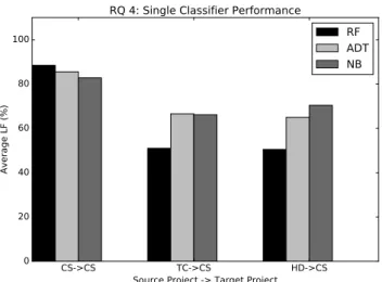
Results: Figure 5 presents the histogram of the average LF values of the RF, ADT and NB classifiers for within-project and cross-project logging predictions for the CloudStack project. Figure 5 shows that the RF classifier provides the highest averageLF of 88.47% for within-project logging prediction. The ADT and NB models provide considerably lower averageLF of 85.54% and 82.81%, respectively, compared to the RF classifier for within-project logging prediction. However, for cross-project logging prediction, the ADT and NB classifiers provide better average LF compared to that of the RF classifier. For ex-ample, for the Hadoop→CloudStack project pair,
NB provides an average LF of 70.42%, which is considerably higher than the average LF of the RF classifier (50.48%). Similar results are observed for other classifiers on other source and
target project pairs (refer to Table 4, Table 5, Table 6 and Table 7 for detailed results). This result shows that algorithms that perform best for within-project and cross-project catch-block logging predictions are different. These results re-veal the weakness of the cross-project logging pre-diction experiment performed by Zhu et al. [11], where the authors perform within-project and cross-project logging predictions using the same algorithm (J48). Hence, in this work, the Au-thors explore multiple classifiers for cross-project catch-block logging prediction model building.
Classifiers that provide the best results for within-project and cross-project logging pre-dictions are different.
Performance summary of base classifiers (RQ1–RQ4): In RO1, 4 investigations are
per-formed in the context of cross-project logging pre-diction. RQ1 indicates that the results of single classifiers are considerably lower for cross-project logging prediction compared to the results for within-project logging prediction. Hence, more advanced methods are required for building the cross-project logging prediction model. RQ2 in-dicates that multi-project training does not im-prove the performance of cross-project logging prediction on all source and target project pairs. Hence, to improve the model building time, only a single project for training the cross-project logging prediction model is considered. RQ3 indi-cates that the classifiers provide complementary information for the task of cross-project logging prediction. Hence, the Authors believe that an ensemble of different classifiers may be beneficial in improving the performance of cross-project logging prediction. RQ4 indicates that the classi-fiers which provide good results for within-project logging prediction are different from the classi-fiers which provide good results for cross-project logging prediction. Hence, to build an ensem-ble of classifiers to improve the performance of cross-project logging prediction, it is necessary to conduct experiments on a wide range of clas-sifiers to find the best set of clasclas-sifiers. The first four RQs derive the motivation for construct-ing the ECLogger model, i.e. an ensemble of classifiers-based model which uses a single project for training the model.
CS->CS TC->CS HD->CS Source Project -> Target Project 0 20 40 60 80 100 Average LF (%)
RQ 4: Single Classifier Performance
RF ADT NB
Figure 5. Performance of RF, ADT, and NB classifiers for within-project and cross-project catch-block logging predictions
6.3. RO2: Performance of
ensemble-based classifiers for cross-project catch-block logging prediction
In this subsection, the performances of ensemble-based classifiers are investigated and compared with the performances of single clas-sifiers for cross-project logging prediction (re-fer to RQ5–RQ8). For each source and target project pair, the single classifier that provides the best results (in terms of average LF) be-comes the baseline classifier. For example, for the CloudStack→Tomcat project pair, the BN
classifier provides the highest average LF and is hence considered to be a baseline classifier (refer to Table 5).
6.3.1. RQ5: What is the performance of ECLoggerBagging for cross-project catch-block logging prediction?
Motivation: In RQ5, the performances of 8 en-semble classifiers, created using the bagging tech-nique, are investigated and compared with the performance of the baseline classifier. The an-swer to this research question can provide impor-tant insights regarding whether bagging is useful in improving the performance of cross-project catch-block logging prediction.
Approach: To answer this research question, the averageLF and average ACC of 8 ensemble
classifiers generated by applying bagging on the base classifiers, i.e. ECLoggerBagging models, are computed. For each source→target project pair,
the bagging model which provides the best av-erageLF is reported. Then the results obtained by the best bagging model is compared with the baseline classifier for each source→target project
pair.
Results: Table 8 presents the average LF and average ACC of the baseline classifier and the best ECLoggerBagging model for each source→target project pair. Table 8 shows that
ECLoggerBagging considerably improves (more than 1% improvement) the averageLF and av-erage ACC for three and two source→target
project pairs, respectively. It improves the av-erage LF and average ACC by 4.6% and 5.57% (CloudStack→Tomcat) and by 3.96% and
2.44% (CloudStack→Hadoop) when BaggingADT
is used. For the Tomcat→CloudStack project
pair, project pair, a considerable improvement (1.03%) is observed only in the average LF. For all other source and target project pairs, no considerable difference in the performance of ECLoggerBagging was observed, compared to the performance of the baseline classifier. Overall, the BaggingADT model performs better than the other bagging models and gives the highest av-erage LF for three source and target project pairs.
ECLoggerBagging shows a considerable im-provement in the average LF in 3 out of 6