Predicting Credit Ratings with Statistical Learning Methods

(1)

Theses and Dissertations (Comprehensive)

2018

Predicting Credit Ratings with Statistical Learning Methods

Yinduo Ma

[email protected]

Follow this and additional works at: https://scholars.wlu.ca/etd

Recommended Citation Recommended Citation

Ma, Yinduo, "Predicting Credit Ratings with Statistical Learning Methods" (2018). Theses and Dissertations (Comprehensive). 2109.

https://scholars.wlu.ca/etd/2109

This Thesis is brought to you for free and open access by Scholars Commons @ Laurier. It has been accepted for inclusion in Theses and Dissertations (Comprehensive) by an authorized administrator of Scholars Commons @ Laurier. For more information, please contact [email protected].

(2)

W

ILFRID

L

AURIER

U

NIVERSITY

M

ASTER

T

HESIS

Predicting Credit Ratings with

Statistical Learning Methods

Author:

Yinduo M

A

Supervisor:

Dr. Roman M

AKAROV

Dr. Xu (Sunny) W

ANG

A thesis submitted in fulfillment of the requirements

for the degree of Master of Science

in the

Department of Mathematics

October 4, 2018

c

(3)

(4)

iii

Declaration of Authorship

I, Yinduo MA, declare that this thesis titled, “Predicting Credit Ratings with Statistical Learning Methods” and the work presented in it are my own. I confirm that:

• This work was done wholly or mainly while in candidature for a re-search degree at this University.

• Where any part of this thesis has previously been submitted for a de-gree or any other qualification at this University or any other institu-tion, this has been clearly stated.

• Where I have consulted the published work of others, this is always clearly attributed.

• Where I have quoted from the work of others, the source is always given. With the exception of such quotations, this thesis is entirely my own work.

• I have acknowledged all main sources of help.

• Where the thesis is based on work done by myself jointly with others, I have made clear exactly what was done by others and what I have contributed myself.

Signed:

(5)

(6)

v

“Do not put your faith in what statistics say until you have carefully considered what they do not say.”

(7)

(8)

vii

Abstract

After the financial crisis in 2008, for many companies, their credit ratings were downgraded to the non-investment grade. People started concerning the reliability of credit ratings. Credit ratings play a vital role in the financial system by balancing information between investors and creditors. It is con-sidered as an essential factor to make financial investment decisions. This thesis is an attempt to determine how to predict credit ratings using the pub-licly available financial information about companies. The data collected are viewed as multivariate high-dimensional financial time series, which have more than one time series and more than one variable to consider. In our re-search, the Dynamic Time Warping (DTW) is used to convert the information contained in the high dimensional time series into a similarity or dissimilar-ity high-dimensional matrix. Then, the Principal Component Analysis (PCA) is used to perform dimension reduction and extract the important informa-tion from the similarity or dissimilarity matrix generated by DTW. Finally, we employ a statistical learning method, namely, the Decision Tree (DT) to predict credit ratings. Furthermore four different scaling methods and sev-eral strategies of increasing the sample size have been considered to improve the prediction accuracy. The most encouraging result is that the predicted credit ratings in the test data have on average at most a two-grade difference with the true credit ratings.

(9)

(10)

ix

Acknowledgements

I would like to thank my supervisors Drs. Roman Makarov and Xu (Sunny) Wang who gave me this interesting topic. Their doors were always open to me whenever I ran into trouble or had questions about my research. They allowed this thesis to be my own work, but they also gave me the right di-rection whenever I needed it.

I would like to thank Dr. Adam Metzler (the second reader) and Dr. Michael Pavlin (the external examiner) for providing valuable comments on this the-sis.

At the end, I would like to thank my parents who are thousands of miles away but have always been my greatest support! Their encouragement helps me through all the years of studies. This achievement would not have been possible without them. Thank you.

(11)

(12)

xi

List of Figures

2.1 Process of Data Cleaning . . . 14

2.2 Overlapping Method . . . 18

3.1 Calculating the correlation between two time series . . . 26

3.2 Sequence Xhas length N = 8, SequenceY has lengthM = 5. (A): Satisfy conditions (1) to (3); (B): Violate boundary condi-tion (1); (C): Violate monotonicity condicondi-tion (2); (D): Violate step size condition (3). . . 27

3.3 Example of Decision Tree. . . 34

(17)

(18)

xvii

List of Tables

1.1 Comparison of three credit rating systems . . . 3

1.2 Long-term rating vs Short-term rating . . . 4

1.3 Variables . . . 7

2.1 The list of 52 companies whose data were analyzed in the thesis 10 2.1 The list of 52 companies whose data were analyzed in the thesis 11 2.1 The list of 52 companies whose data were analyzed in the thesis 12 2.2 Grouping 52 Companies based on credit ratings . . . 13

2.3 Summary of companies in four credit rating grades . . . 15

2.4 Common variables . . . 16

2.5 Five different splits . . . 20

2.6 Example of distance measure calculation . . . 21

2.7 Example of 4 grades . . . 22

3.1 The Final Data Set . . . 38

4.1 Common Variables with 10 Grades . . . 40

4.2 All Variables with 10 Grades . . . 42

4.3 Common Variables with 4 Grades . . . 43

4.4 All Variables with 4 Categories . . . 44

4.5 Results without any transform with 10 Grades . . . 46

4.6 Results for the transform _stdx₍_X₎ with 10 Grades . . . 47

4.7 Results for the transform _max₍_absx ₍_X₎₎ with 10 Grades . . . 48

(19)

4.9 Results for the transform _stdx−₍_XX¯₎ with 10 Grades . . . 49

4.10 Comparison of all the methods with 10 grades . . . 50

4.11 Results without any Transform with 4 Grades. . . 51

4.12 Results for the transform _stdx₍_X₎ with 4 Grades . . . 52

4.13 Results for the transform _max₍_absx ₍_X₎₎ with 4 Grades . . . 52

4.14 Results for the transform _maxx₍−_Xmin₎₋_min(X)₍_X₎ with 4 Grades . . . 53

4.15 Results for the transform _stdx−₍_XX¯₎ with 4 Grades . . . 54

4.16 Comparison of all the methods with 4 Grades . . . 54

4.17 Overlapping data with 10 Grades . . . 56

4.18 Overlapping data with 4 Grades . . . 57

4.19 104 companies with 10 Grades . . . 58

4.20 104 companies with 4 Grades . . . 59

4.21 Results of Different Year Rating Comparison . . . 60

4.22 Results of Total 0 . . . 61 4.23 Results of Total 1 . . . 61 4.24 Additional 5 splits. . . 62 A.1 52 Companies . . . 67 A.1 52 Companies . . . 68 A.1 52 Companies . . . 69

(20)

xix

List of Abbreviations

DTW DynamicTimeWarping

PCA PrincipalComponentAnalysis

DT DecisionTree

CV CommonVariables Method

AV AllVariables Method

(21)

(22)

xxi

(23)

(24)

1

Chapter 1

Introduction

1.1 Corporate Credit Ratings

The importance of corporate credit rating in the financial market is needless to argue. A corporate credit rating is an independent opinion from an in-dependent third party regarding the corporate financial situation. It is an indicator of whether a company will meet its financial obligations as they come due. Therefore creditors usually use credit ratings as a tool to assess a company’s ability to pay back loans. The corporate credit rating suggests investors how financial instruments of a company such as debt securities should be priced in term of yields. Hence a credit score has become a pri-mary reference to make financial decisions. A credit rating file is a detailed report based on the financial history of borrowing or lending and creditwor-thiness of the entity obligations, defined rating methodologies, and rating criteria. The relative credit rating is given by letter grade or number grade symbols.

There are many agencies that evaluate a company’s financial situation. The three largest agencies worldwide are Moody’s Investors Service, Standard & Poor’s and Finch. These three agencies control 85% of the market, which means 85% companies are evaluated by these three agencies. Each agency has its own rating system, which is confidential. The rating scales are not

(25)

necessarily identical to each other, but they are similar. Credit ratings have two categories: short-term ratings and long-term ratings. Short-term rat-ings are the opinions of the ability of issuers to honour short-term financial obligations. Such financial obligations expire within thirteen months unless explicitly noted [13]. Long-term ratings are the opinions of the relative credit risk of financial obligations with an original maturity of one year or more [13]. The corporate credit rating is not a guarantee that the company will pay its financial debts off. In the long run, the changing trend of corporate credit ratings distinguishes the financial situation among rated companies. There-fore, in this thesis, we focus on predicting the long-term credit ratings using a company’s financial report over a 10-year period.

Table1.1 presents the credit ratings from the three largest agencies. In this thesis we only focus on Moody’s Investors Service credit rating scale. In terms of the investment grade, there are 10 different categories. Aaa is the highest grade, the next best areAa1toAa3, then followed byA1toA3, down to Baa1toBaa3. In the non-investment grade,Bais the highest grade down toCa, andCis considered as the default grade. Standard & Poor’s and Finch have a similar credit rating scale. Standard & Poor’s and Finch use AAA

as the highest credit rating, the next best isAA, then followed by A, down to BBB which are all considered as the investment grades. Everything be-lowBBBis considered as the non-investment grade speculative, down toD, which is considered as the default grade. In this thesis, we only consider the investment grades:

This thesis is an attempt to determine how the financial information collected affects the ratings using statistical learning and data mining techniques.

(26)

1.2. Moody’s Investors Service Credit Rating 3

TABLE1.1: Comparison of three credit rating systems

Moody’s Investors Service Standard & Poor’s Finch Investment Grade

Aaa AAA AAA

Aa1, Aa2, Aa3 AA+, AA, AA- AA+, AA, AA-A1, A2, A3 A+, A, A- A+, A, A-Baa1, Baa2, Baa3 BBB+, BBB, BBB- BBB+, BBB,

BBB-Non-investment Grade

Ba1, Ba2, Ba3 BB+, BB, BB- BB+, BB, BB-B1, B2, B3 B+, B, B- B+, B, B-Caa1, Caa2, Caa3 CCC+, CCC, CCC- CCC+, CCC,

CCC-Ca CC CC

C C

C D D

1.2 Moody’s Investors Service Credit Rating

Since 1909 when John Moody published the first debt ratings in the Manual of Railroad Securities, the Moody’s Investors Service rating has been popular in the U.S. bonds market. Based on maturity time of debt securities, Moody’s Investors Service offers both short-term credit rating and long-term credit rating.

Based on Moody’s Investors Service, the short-term rating refers to an opin-ion in terms of debt securities with maturity time less than one year. It has four categories:Prime-1,Prime-2,Prime-3, down toNot Prime. Prime-1, Prime-2 and Prime-3 are investment grades, Not Primeis a non-investment grade. Moody’s long-term rating refers to an opinion in terms of debt securities with maturity time more than one year. There are twenty-one categories starting from the highestAaa to the lowest C. In the investment grade, there are 10 different categories among whichAaais the highest grade, the next best are

Aa1 toAa3, then followed by A1 to A3, down to Baa1 toBaa3. In the non-investment grade, there are 11 different categories, among which Ba is the highest grade, then down to Ca, and C is considered as the default grade.

(27)

The summary and relationship between the short-term rating and the long-term rating is shown in Table1.2.

TABLE1.2: Long-term rating vs Short-term rating

Long-term Rating Short-term Rating

Investment Grade Aaa Prime-1 Aa1 Aa2 Aa3 A1 A2 A3 Prime-2 Baa1 Baa2 Prime-3 Baa3 Non-investment Grade

Ba1, Ba2, Ba3

Not Prime B1, B2, B3

Caa1, Caa2, Caa3 Ca, C

Next, we want to list the information that Moody’s Investors Service uses to decide credit ratings [13].

• Publicly available data, e.g., annual reports.

• Market data, e.g., stock price trends, trading volumes, data on bond price spreads.

• Prospectuses, offering circulars, offering memoranda, trust deeds, or indentures of particular securities.

• Economic data from industry groups, associations, e.g., the World Bank. • Data from agencies, e.g., central banks, ministries, or regulators.

• Books or articles from academic sources, financial journals, news re-ports.

(28)

1.3. Literature Review 5 • Discussions with experts in industry, government or academia.

• Data that come from meetings or conversations of debt issuers.

As some information is not easy to obtain, in our research we decide to use publicly available market data fromBloomberg–financial terminal.

1.3 Literature Review

Previous studies show that supervised statistical learning methods can sig-nificantly improve the prediction accuracy. The authors in [6] developed a two-stage statistical learning method to improve the prediction accuracy of credit score rating. They used feature selection, data clustering, and data resampling as stage-one learning methods to process data. Then they em-ployed supervised learning methods such as decision tree, artificial neural networks and support vector machines as stage-two methods to model data and perform predictions. The authors in [1], [9], [8] also described several supervised statistical learning methods such as decision tree and logistic re-gression for financial data prediction. However, there are two main limita-tions in the current studies. The first limitation is the use of a single-variate time series. For instance, the data have one variable withn observations for 20 years. The second limitation is the use of multivariate data at one time point. For example, the data may contain 20 variables withnobservations at year 2017.

The aim of this research is to determine how the financial information col-lected affects the credit rating by analysing multivariate high-dimensional financial time series including the information from Balance Sheet, Income Statement, Cash Flow Statement, Financial Ratios, Options and Employment

(29)

Data.

1.4 Data

According to Moody’s Analysis, the Balance Sheet, Cash Flow Statement, Financial Ratios such as Liquidity are important to assess corporate credit ratings [4]. All the financial statements are adjusted on a relative accounting standard. In our research, we want to use as much financial information as possible when building a model, so we include not only the Balance Sheet, Cash Flow Statement, Financial Ratios like Liquidity but also Income State-ment, Options, Employment Data and Financial Ratios such as Profitability, Growth, Credit, and Working Capital. We collect 10-year financial data from years 2008 to 2017 for 52 companies. Each company has more than 300 vari-ables and the total number of varivari-ables is not the same for all companies. The variables from Balance Sheet, Income Statement, Cash flow Statement, Fi-nancial Ratios, Options and Employment Data are summarized in Table1.3. Modeling this large data set is challenging as it is a typical large P (dimen-sions) and small n (sample size) problem. The data are multivariate high-dimensional time series because each company has more than 300 variables and each variable is a time series for 10 years.

1.5 Methodology

As mentioned in Section 1.4, in order to make accurate predictions, we use multivariate high-dimensional financial time series that include the informa-tion from balance sheets, working capital data, etc. It is not easy to apply any statistical learning and data mining method to such high-dimensional time series data directly. In our research, the Dynamic Time Warping (DTW) is

(30)

1.5. Methodology 7 TABLE1.3: Variables Income Statement: SALES_REV_TURN IS_SALES_AND_SERVICES_REVENUES IS_COGS_TO_FE_AND_PP_AND_G IS_COG_AND_SERVICES_SOLD GROSS_PROFIT . . . . Balance Sheet: C&CE_AND_STI_DETAILED BS_CASH_NEAR_CASH_ITEM BS_MKT_SEC_OTHER_ST_INVEST BS_ACCT_NOTE_RCV BS_ACCTS_REC_EXCL_NOTES_REC . . . .

Cash Flow Statement:

CF_CHNG_NON_CASH_WORK_CAP CF_ACCT_RCV_UNBILLED_REV CF_CHANGE_IN_INVENTORIES CF_CHANGE_IN_ACCOUNTS_PAYABLE INC_DEC_IN_OT_OP_AST_LIAB_DETAIL . . . . Options: BS_OPTIONS_GRANTED BS_OPTIONS_EXERCISED BS_OPTIONS_CANCEL_FORFEIT_EXPRD BS_OPTIONS_CANCELLED_FORFEITED BS_OPTIONS_ADJUSTMENT . . . . Employment Data: NUM_OF_EMPLOYEES EMPL_GROWTH ACTUAL_SALES_PER_EMPL ACTUAL_NET_INCOME_PER_EMPLOYEE ACTUAL_ASSETS_PER_EMPLOYEE . . . . Financial Ratios: Profitability: RETURN_COM_EQY RETURN_ON_ASSET RETURN_ON_CAP RETURN_ON_INV_CAPITAL . . . . Growth: SALES_GROWTH EBITDA_GROWTH OPER_INC_GROWTH EARN_FOR_COM_GROWTH . . . . Credit : SHORT_AND_LONG_TERM_DEBT BS_ST_BORROW BS_LT_BORROW . . . . Liquidity: CASH_RATIO CUR_RATIO QUICK_RATIO CFO_TO_AVG_CURRENT_LIABILITIES . . . . Working Capital: ACCT_RCV_TURN ACCT_RCV_DAYS INVENT_TURN INVENT_DAYS . . . .

used to convert the information from high dimensional time series to a “simi-larity/dissimilarity” matrix. Then, the Principal Component Analysis (PCA) is used to reduce the dimensionality and extract important information from the “similarity/dissimilarity” matrix. Finally, we employ a supervised sta-tistical learning method, namely, Decision Tree (DT), to predict credit scores.

(31)

1.6 Thesis Structure

The thesis is organized as follows. Chapter2introduces the structure of data, the data cleaning and four different scaling methods. The model evaluation criterion and the several experimental designs are the most important part in Chapter 2. Chapter3 introduces the methodologies employed in the thesis such as the Dynamic Time Warping (DTW), the Principal Component Anal-ysis (PCA) and the Decision Tree (DT). Chapter4 presents the experimental results. Chapter 5 summarizes the whole thesis and provides some future research directions.

(32)

9

Chapter 2

High-dimensional Time Series

Financial Data

In this Chapter, the Section2.1gives the details on the structure of data and the data cleaning method. The Section 2.2 gives the reasons why we re-group the data. There are three comparison strategies described in Section

2.3. We introduce the prediction accuracy improvement strategies in Section

2.4. Then Section2.5entails the training and test sets. Section2.6introduces the model evaluation criterion.

2.1 Structure of Data

We collect the financial information over a 10-year period from 2008 to 2017 for 52 companies. The financial information collected comes from Balance Sheets, Income Statements, Cash Flow Statements, Options and Employment Data and Financial Ratios such as Profitability, Growth, Credit, and Working Capital. The company names and tickers along with their credit ratings are summarized in Table2.1. The data for each company contain more than 300 variables. The total number of variables is not the same for every company.

(33)

TABLE2.1: The list of 52 companies whose data were analyzed in the thesis

Credit Rating Company Name (Ticker)

Aaa

Federal Home Loan Mortgage Co. (FMCC) Exxon Mobil Co. (XOM)

Johnson & Johnson (JNJ) Microsoft Co. (MSFT)

Tennessee Valley Authority (3015A) Aa1 Apple Inc. (AAPL)

St Galler Kantonalbank AG (SGKN)

Aa2

Berkshire Hathaway Inc. (BRK) Chevron Co. (CVX)

Royal Dutch Shell PLC (RDSA) Nestle SA (NESN)

Walmart Inc. (WMT)

Aa3

Canon Inc. (CAJ) Coca-Cola Co. (KO) Toyota Motor Co. (7203) Procter & Gamble Co. (PG) TOTAL SA (FP)

A1

International Business Machines Co. (IBM) Intel Co. (INTC)

Cisco Systems Inc. (CSCO) 3M Co. (MMM)

Merck & CO., Inc. (MRK) Nike Inc. (NKE)

Pfizer Inc. (PFE) Visa Inc. (V)

(34)

2.1. Structure of Data 11

A2

Axactor AB (AXA) Walt Disney Co. (DIS) General Electric Co. (GE) Home Depot Inc. (HD) Boeing Co. (BA)

A3

Volkswagen AG (VOW) Caterpillar Inc. (CAT)

EI du Pont de Nemours & Co. (DD) Goldman Sachs Group Inc. (GS) JPMorgan Chase & Co. (JPM) United Technologies Co. (UTX) Phillips 66 (PSX)

Baa1

Citigroup Inc. (C) McDonald’s Co. (MCD)

Mondelez International Inc. (MDLZ) Verizon Communications Inc. (VZ) AT&T Inc. (T)

Baa2

Ford Motor Co. (F)

Boston Scientific Co. (BXS) E.ON SE (EOAN)

Kirby Co. (KEX)

Nordic Group Ltd (NRD)

Baa3

Andeavor (ANDV) DDR Co. (DDR)

(35)

General Motors Co. (GM) TDC A/S (TDC)

Based on the Dow Jones Industrial Average Index (DJIA), we first col-lected the financial information for 30 companies included by the (DJIA) in-dex. Then we collected 10-year Moody’s Investors Service long-term credit ratings for those 30 companies. These companies are grouped based on their 2017 credit ratings. The long-term credit ratings for those 30 companies be-long to the investment grade. The credit ratings fall into A1 or A3 for the majority of the companies. While keeping all 30 companies, we collected data for additional 22 companies with attempt to have minimum 5 com-panies in each investment grade. Those comcom-panies are selected based on Moody’s long-term credit rating for 2017. However, we were able to gather only two companies’ financial information for gradeAa1. The detailed sum-mary of credit rating grades and corresponding companies within each grade are shown in Table2.2.

2.1.1 Data Cleaning

The data collected are not ready to use yet as they contain a lot of missing values. For each variable and each company, there are a maximum of 10 observations. Therefore, if the number of missing values for some variable exceeds 5, this variable should be removed. If we imputed a variable with more than 5 missing values, the imputation result would be inaccurate. We simply use the mean imputation method to impute the variables with less

(36)

2.1. Structure of Data 13

TABLE2.2: Grouping 52 Companies based on credit ratings

Grade Ticker

Aaa (5) FMCC, JNJ, MSFT, 3015A, XOM

Aa1 (2) AAPL, SGKN

Aa2 (5) BRK, CVX, RDSA, NESN, WMT Aa3 (5) CAJ, KO, 7203, FP, PG

A1 (8) CSCO, IBM, INTC, MMM, MRK, NKE, PFE, V,

A2 (5) AXA, DIS, GE, HD, BA

A3 (7) CAT, DD, GS, JPM, PSX, UTX, VOW Baa1 (5) C, MCD, MDLZ, T, VZ

Baa2 (5) BXS, F, EOAN, KEX, NRD, Baa3 (5) ANDV, DDR, ENELAM, GM, TDC

than 5 missing values. Furthermore, we discovered that some variables have the exactly same value for all 10 years. All the variables without variation are removed as well. Additionally, we realized that the magnitude of vari-ables is different. For instance, the revenue has a value 39,540 with the order of magnitude 5, whereas the fixed asset has a value 6.23 with the order of magnitude 1. If these two variables are equally important, the variable with a large magnitude may have a bigger influence than the variable with a small magnitude in the model. We propose several scaling methods to transform variables in order to bring them to the same magnitude.

The four scaling methods proposed are listed in formulae (2.1)-(2.4). LetXbe a variable,Xthe mean,std(X)the standard deviation,min(X)the minimum value,max(X)the maximum value,abs(X)the absolute value andxis a par-ticular value of variableX. In all formulae we use sample values calculated using 10-year data.

1. Subtract the mean of the variable and divide by its standard deviation:

x−X

(37)

2. Divide by the standard deviation of this variable:

x

std(X) (2.2)

3. Subtract the minimum value and divide by the difference between the maximum value and the minimum value:

x−min(X)

max(X)−min(X) (2.3)

4. Divide by the maximum absolute value of this variable:

x

max(abs(X)) (2.4)

Original Data Set Delete Variables with more

than 5 missing values Impute Data by Mean Imputation

Delete Variable without Variation Rescale Variables Data Set Ready-to-use

(38)

2.2. Data Regrouping 15

2.2 Data Regrouping

As mentioned in Section 2.1, we collected data for 52 companies in total and we tried to have 5 companies for each grade. The sample size is small, es-pecially inAa1 where there are only two companies. Moody’s credit rating system includes 3 bigger groups: Aa: (Aa1, Aa2, Aa3), A: (A1, A2, A3), Baa: (Baa1, Baa2, Baa3). The difference between ratings within each group is not significant. To improve the sample size, the companies from adjacent grades are regrouped by combining the companies with ratingsAa1, Aa2, Aa3into GroupAb, those with ratingsA1, A2, A3in GroupAcand those with ratings

Baa1, Baa2, Baa3in GroupBa, leaving Aaaas a single group. The details are shown in Table2.3. In this thesis, we consider: 10-grade and 4-grade classifi-cation problems.

TABLE2.3: Summary of companies in four credit rating grades

Categories Ticker

Aaa (5) FMCC, JNJ, MSFT, 3015A, XOM

Ab (12) AAPL, SGKN, BRK, CVX, RDSA, NESN, WMT CAJ, KO, 7203, FP, PG

Ac (20)

CSCO, IBM, INTC, MMM, MRK, NKE, PFE, V, AXA, DIS, GE, HD, BA, CAT, DD,

GS, JPM, PSX, UTX, VOW Ba (15)

C, MCD, MDLZ, T, VZ, BXS, F, EOAN, KEX, NRD,

ANDV, DDR, ENELAM, GM, TDC

Since each company has more than 300 variables and the total number of variables in each company is different, it is difficult to list all the variables. The common variables are extracted from 52 companies. These common variables can be used to perform prediction. The 60 common variables are listed in Table2.4. Those common variables appear among all 52 companies.

(39)

TABLE2.4: Common variables Income Statement IS_OPER_INC IS_TOT_CASH_PFD_DVD PRETAX_INC OTHER_ADJUSTMENTS IS_ABNORMAL_ITEM EARN_FOR_COMMON PRETAX_INC.1 EARN_FOR_COMMON.1 IS_INC_TAX_EXP IS_NET_ABNORMAL_ITEMS IS_INC_BEF_XO_ITEM XO_GL_NET_OF_TAX.1 XO_GL_NET_OF_TAX OPER_MARGIN IS_DISCONTINUED_OPERATIONS PROF_MARGIN IS_EXTRAORD_ITEMS_._ACCTG_CHNG ACTUAL_SALES_PER_EMPL NI_INCLUDING_MINORITY_INT_RATIO NET_INCOME MIN_NONCONTROL_INTEREST_CREDITS Balance Sheet BS_CASH_NEAR_CASH_ITEM TOTAL_EQUITY BS_TOT_ASSET BS_FUTURE_MIN_OPER_LEASE_OBLIG BS_PFD_EQTY_._HYBRID_CPTL NET_DEBT MINORITY_NONCONTROLLING_INTEREST NET_DEBT_TO_SHRHLDR_EQTY

Cash Flow Statement

CF_NET_INC CF_INCR_CAP_STOCK CF_CASH_FROM_OPER CF_DECR_CAP_STOCK CF_CASH_FROM_INV_ACT CF_NET_CHNG_CASH CF_DVD_PAID FREE_CASH_FLOW_EQUITY Credit SHORT_AND_LONG_TERM_DEBT LT_DEBT_TO_TOT_ASSET TOTAL_DEBT_TO_EBIT TOT_DEBT_TO_TOT_EQY NET_DEBT_TO_EBIT TOT_DEBT_TO_TOT_CAP COM_EQY_TO_TOT_ASSET TOT_DEBT_TO_TOT_ASSET LT_DEBT_TO_TOT_EQY NET_DEBT_._CAPITAL LT_DEBT_TO_TOT_CAP Liqudity COM_EQY_TO_TOT_ASSET.1 TOT_DEBT_TO_TOT_EQY.1 LT_DEBT_TO_TOT_EQY.1 TOT_DEBT_TO_TOT_CAP.1 LT_DEBT_TO_TOT_CAP.1 TOT_DEBT_TO_TOT_ASSET.1 LT_DEBT_TO_TOT_ASSET.1 CASH_FLOW_TO_TOT_LIAB Employ Data EMPL_GROWTH NUM_OF_EMPLOYEES Response variable

Long term credit rating

2.3 Comparison Strategies

2.3.1 Common Variables vs All variables

We consider all ten-year financial information with the scaling methods in-troduced in Section2.1.1. There are 60 common variables extracted and listed in Table2.4. We want to compare the prediction results of two experiments: including only common variables and including all the variables. The out-come will determine whether we should use the common variables only or

(40)

2.3. Comparison Strategies 17 all variables. We choose theMean and Standard Deviationscaling method, for both 10-grade and 4-grade tests. The results are presented in Chapter4.

2.3.2 Scaling Methods

Next, since variables have different magnitudes, we propose several scaling methods in order to have the same magnitude for all variables. In order to save computing time, we use only 5-year financial information from 2013 to 2017 to compare 4 scaling methods. The purpose of this step is to determine which scaling method is the best for data in 10 grades and in 4 grades.

2.3.3 10-year Financial Information vs 5-year Financial

Infor-mation

Lastly, we wish to know whether the prediction accuracy can be improved by including financial information for a long period of time. We compare the results with 10-year financial data to those with 5-year financial information using the same scaling method. The result are shown in Chapter4.

Common Variables vs All Variables

Selection of Scaling Method

(41)

2.4 Strategies of Improving Prediction Accuracy

Strategy 1:

The sample size is really small, and we hence want to fully use the informa-tion contained in the data. The first strategy is to use all 10-year data. We start with the first 5-year data (2008-2012), then the next 5-year data (2009-2013) and keep going until the last 5-year (2013-2017). This process is called the Overlapping Method (OM) demonstrated in Figure2.2. For each 5-year data we apply the techniques described in Chapter 3 to get the first 20 principal components (PCs). The final data set consists of 120 PCs as input variables and the 2017 credit ratings as response variables. The aim of this strategy is to improve the prediction result by incorporating as much information from the data as possible.

(42)

2.5. Training and Test Sets 19

Strategy 2:

It is a challenging task for us to find more companies, which have the high level investment grade likeAaa, Aa1, but we still want to increase the sample size. As we know, a company’s financial situation may change a lot during 10 years. Meanwhile, the most of the missing values occur within the first 5 years. For each company, we can use the first 5 years as one sample, and then the last 5 years as another sample.This way we can get 104 samples in total. The outcome from this strategy can tell us if more samples can improve the prediction accuracy.

2.4.1 Examination of Credit Rating Delay Effect

The last numerical test is to check whether the credit rating has a delay effect or not. We use the first 5-year data (2008-2012) to predict credit ratings. Then we compare the results with the true credit ratings in Year 2012, 2013,..., 2017 to examine the prediction accuracy and check whether there is a delay effect.

2.5 Training and Test Sets

A training set is used to build the model. A test set is used to test the model. A model can fit training data equally well, but probably can not fit test data very well. This effect is called overfitting. We pay more attention to the pre-diction results based on test data. We decide to use an 80 : 20 ratio to split data into training and test sets. Thus, there are 42 companies in the train-ing set and 10 companies in the test set. The companies in the test set are randomly selected within each grade as we want to have one company from each grade.

(43)

The data are divided into training and test sets based on credit rating grades. Similar to theK-fold cross validation, we run each experiment 5 times so that every company can be included in the test set once. Each time the company indexes in the test set are different.

We use the same training and test sets for all experiments. Since the sample size is really small, changing the companies in the test set can significantly affect prediction results. There are only two companies in gradeAa1, so we alternatively include one in the training set and the other in the test set. The 5 random splits for the test sets are shown in Table2.5.

TABLE2.5: Five different splits

Test Company Index

Split 1 50, 52, 49, 44, 47, 22, 51, 48, 35, 42 Split 2 18, 2, 5, 8, 10, 1, 9, 7, 6, 3 Split 3 25, 52, 11, 28, 23, 14, 21, 29, 16, 13 Split 4 33, 2, 39, 37, 24, 14, 26, 30, 17, 15 Split 5 45, 2, 40, 43, 34, 19, 38, 41, 27, 20

2.6 Model Evaluation Criterion

2.6.1 Ten Grades

Since the sample size is small (only 52 companies) we can not expect that our prediction results are exactly as same as Moody’s ratings. If the pre-dicted credit rating differs from the true credit rating by only one grade, we can say that our prediction result is really good. Recall that the credit rat-ing is between the highest ratrat-ing gradeAaaand the lowest grade Baa3. We use distance to measure the difference between the true credit rating and the

(44)

2.6. Model Evaluation Criterion 21 predicted one: the smaller value of the distance measure is, the better the prediction results are. For instance, the first column of Table2.6, shows the true credit ratings as letters; the second column shows the numerical values of the true credit ratings; the third column contains a set of possible predicted values and the last column the distances between the true and the predicted ratings.

TABLE2.6: Example of distance measure calculation

Letter Rating Assigned Numerical Value Predicted Value Distance Measure

Aaa 1 5 4 Aa1 2 5 3 Aa2 3 5 3 Aa3 4 6 2 A1 5 5 0 A2 6 10 4 A3 7 1 6 Baa1 8 3 5 Baa2 9 3 6 Baa3 10 5 5 Total - - 38 Average - - 3.8

We calculate the difference between the true credit rating and the prediction result. For example, if the true number credit rating is Aaa, which corre-sponds to a numerical value 1, and the predicted value isA1corresponding to a numerical value 5, then the distance between the two ratings is 4. The distance is calculated for all prediction results, and then the average distance is used as the final result for comparison. For example the total distance in Table2.6is 38, and the average distance is 3.8, i.e., 38/10=3.8.

LetYi represent the true credit rating value and ˆYi the predicted value. The

average distance is calculated as:

D = ∑

m

i=1|Yi−Yiˆ|

(45)

where mis the number of companies in the test set. We repeat this process for all 5 random splits and calculate the final overall average prediction error.

2.6.2 Four Grades

We leaveAaaon its own. The gradesAa1, Aa2, Aa3are considered in group

Ab;A1, A2, A3form groupAc; andBaa1, Baa2, Baa3are included in groupBa. The difference between four grade groups and ten grades is how to assign a numerical value to each group. We use the average assigned value for each new group. For example, in Table2.7, the first column is the true group credit rating in the letter form, the second column is the average numerical ratings for each new group.

TABLE2.7: Example of 4 grades

Group Letter Rating Assigned Numerical Value Predicted Value Distance Measure

Aaa 1 6 5 Ab 3 3 0 Ab 3 3 0 Ab 3 6 3 Ac 6 6 0 Ac 6 6 0 Ac 6 6 0 Ba 9 3 6 Ba 9 3 6 Ba 9 9 0 Total - - 20 Average - - 2.0

Based on the 10 grades, the assigned numerical value for gradeAa1is 2, for gradeAa2is 3, for gradeAa3is 4, then the average value for the new grade

Abis 3. Similarly, the assigned value for gradeAcis 6, and for gradeBais 9. The third column is a possible set of prediction results for 4 categories. The last column lists the calculated differences between the true and predicted ratings. In this case, forAaa, the distance between the true credit rating and the predicted credit rating is 5. Repeating this process for all categories gives

(46)

2.6. Model Evaluation Criterion 23 the total distance 20 and the average distance 2. We repeat the whole process 5 times for different splits to calculate the overall average prediction error.

(47)

(48)

25

Chapter 3

Methodology

In this thesis we consider data as multivariate high-dimensional financial time series. It is not easy to apply any statistical learning and data min-ing method to multivariate high-dimensional time series directly. In our research, the dynamic time warping (DTW) is used to convert the informa-tion from dimensional time series into a similarity/dissimilarity high-dimensional matrix. Then, the principal component analysis (PCA) is used to reduce the dimensionality and extract the important information from the similarity/dissimilarity matrix. Finally, we employ statistical learning meth-ods such as the Decision Trees (DT) to make predictions.

3.1 Dynamic Time Warping

The Dynamic time warping (DTW) is a well-known technique to find an op-timal alignment between two time-dependent sequences. There exist tra-ditional methods to handle time series such as Autoregressive Integrated Moving Average (ARIMA), Autoregressive Conditional Heteroskedasticity

(ARCH) and Generalized Autoregressive Conditional Heteroskedasticity (GARCH). All these methods can only handle a single time series at a time. Because

our data are high-dimensional, all these traditional methods can not be ap-plied here and thus DTW becomes our primary method. As demonstrated in

(49)

Figure3.1(A), usually, we can only calculate the correlation between two se-quences correspondingly. However, DTW allows us to shift time to calculate the correlation between two unaligned time-dependent sequences as show-ing in Figure3.1(B).

(A) Traditional Way

(B) Dynamic Time Warping

FIGURE3.1: Calculating the correlation between two time se-ries

Consider two time-dependent sequencesX := (x1,x2, ...,xN)of lengthNand

Y := (y1,y2, ...,yM)of lengthM. The local distance measurec(x,y)is defined as similarity of each pair of elements between the sequencesXandY:

• Ifxandyare similar to each other,c(x,y)is small; • Ifxandyare not similar to each other,c(x,y)is large.

The local distance matrixC(X,Y) is obtained by calculating c(x,y) for each pair of elements from the sequencesX andY. An(N,M)-warping path is a sequencep = (p1, ...pL)with pl = (nl,ml) ∈ [1 : N]×[1 : M]forl ∈ [1 : L]

that must satisfy three conditions:

(50)

3.1. Dynamic Time Warping 27 2. Monotonicity condition: n1 ≤n2 ≤...≤nL andm1 ≤m2 ≤... ≤mL;

3. Step size condition: pl+1−pl ∈ {(0, 1),(1, 0),(1, 1)} forl ∈ [1 : L−1]

(A) (B) (C) (D)

FIGURE 3.2: Sequence X has length N = 8, Sequence Y has length M = 5. (A): Satisfy conditions (1) to (3); (B): Violate boundary condition (1); (C): Violate monotonicity condition (2);

(D): Violate step size condition (3).

The total distancecp(X,Y)of a warping path pbetweenXandYwith respect

to the local distancecis defined as

cp(X,Y) := L

∑

l=1

c(xn_l,ym_l)

The optimal distance is

DTW(X,Y) =min{cp(X,Y)| p is an (N,M)−warping path}

A Toy Example of Dynamic Time Warping:

Consider the following two sequences:

X := (α,β,γ),Y := (α,β,β,γ). Assume if x = y, c(x,y) = 0 otherwise

c(x,y) =1. What is DTW(X,Y)?

(51)

p1 ={(α,α),(α,β),(β,β),(γ,γ)}withcp(X,Y) =1

p2 ={(α,α),(β,β),(β,β),(γ,γ)}with cp(X,Y) = 0

p3 ={(α,α),(α,β),(β,γ),(γ,γ)}with cp(X,Y) =2

Therefore, the optimal distance isDTW(X,Y) =0 [11]. We should be aware that the warping path whose total distance equals the optimal distance may not be unique.

3.1.1 Optimal Distance Algorithm

We could try every possible path between Xand Yto find the optimal path

p∗. However, as the lengths of X and Y increase, the intensity of computa-tion will increase exponentially. AnO(N M)algorithm is designed based on dynamic programming that can solve this optimal distance problem.

We define the prefix sequences X(1 : n) := (x1,x2, ...,xn) for n ∈ [1 : N] andY(1 :m) := (y1,y2,y3, ...,ym)form ∈ [1 : M]and set theaccumulated cost

matrix(D(n,m)) with dimensions N×Mas

D(n,m):=DTW{X(1 :n),Y(1 :m)} (3.1)

The elementD(N,M)is equal to DTW(X,Y). The next theorem guarantees that allD(n,m)can be computed efficiently.

Theorem3.1.1: The accumulated cost matrix(D(n,m)) satisfies the following identities: D(n, 1) = _∑n_k₌₁c(xk,y1) forn ∈ [1 : N], D(1,m) = ∑km=1c(x1,yk)

form ∈[1 : M], and

(52)

3.2. Principal Component Analysis 29 for 1<n≤ Nand 1<m≤ M. In particular,DTW(X,Y) = D(N,M)can be computed withO(N M)operations.

The optimal warping path p∗ = (p1, ...,pL) is computed in reverse order of the indices starting with pL = (N,M). Suppose Pl = (n,m) has been

com-puted. In case (n,m) = (1, 1), one must have l = 1 and the procedure is finished. Otherwise, pl−1:=                (1,m−1), if n =1; (n−1, 1), if m =1; argmin{D(n−1,m−1),D(n−1,m),D(n,m−1)}, otherwise; where we take the lexicographically smallest pair in case “argmin” is not unique.

3.2 Principal Component Analysis

The Principal Component Analysis (PCA) is a popular dimension reduction method dating back to 1901. Assume there is a data set withnobservations and f features. We can check the two-dimensional scatterplots which contain many pairs ofn observations’ features. There are f(f −1)/2 scatterplots in total. If f is large, it is impossible for us to check every two-dimensional scat-terplot. Even if we can check all scatterplots, the information gathered is not complete. Each time we can only examine a small number of features of the data set. In this case, we need a better statistical tool to perform dimension reduction.

(53)

data with a smaller number of representative variables that collectively ex-plain most of the variability in the original data set. Therefore, PCA refers to the process by which principal components are computed, and then uses these components in understanding data. Each of the new dimensions found by PCA is a linear combination of all features.

Assume a data set hasnobservations and f features X1, ...,Xf. Theith

prin-cipal component is defined asZiwritten as

Zi =φ1iX1+φ2iX2+...+φf iXf, (3.3)

wherei =1, ..., f, and(φ1i, ...,φpi)T is called the principal component loading

vector of theith principal component.

3.2.1 Principal Component Analysis Algorithm

The first principal componentof a set of featuresX1,X2, ...,Xf is the normalized

linear combination of the features, which can be written as

Z1 =φ11X1+φ21X2+...+φf1Xf, (3.4)

where “normalized" means that ∑_jf₌₁φ2_j₁ = 1. The first PC has the largest

variance and can be found by solving the optimization problem written in (3.5), max φ11,...,φf1 n1 n n

∑

i=1 f

∑

j=1 φj1xij 2o subject to f

∑

j=1 φ2_j₁ =1. (3.5)

We can use a similar procedure to find the rest of principal components given these principal components are orthogonal to each other.

(54)

3.2. Principal Component Analysis 31 An alternative approach to this optimization problem is to find eigenvalues of the sample covariance matrix.

Step 1. Subtract the mean of each variable.

Step 2. Calculate the covariance matrix.

Step 3. Calculate eigenvalues and eigenvectors of the covariance matrix.

Step 4, Select the number of eigenvalues given the percentage of the cumu-lative variance explained by the eigenvalues selected.

Both approaches require scaling variables first because unscalled variables will significantly affect the outcome. In this thesis, we will try different ing methods and then compare all those methods with the case without scal-ing to determine which scalscal-ing method can give a better prediction result.

3.2.2 Selection of Principal Components

After principal components are calculated, we need to determine the proper number of principal components for further analysis. The goal of the appli-cation of PCA in our research is to extract the important information from a high dimensional matrix. We use theproportion of variance explained (PVE) to determine the number of principal components. The PVE of theith principal component is calculated by formula (3.6),

∑n i=1(∑ f j=1φjixij)2 ∑_jf=1∑ n i=1x2ij . (3.6)

We use the smallest possible number of principal components that explain the most variation of the data. However, there is no universal rule to decide what number of principal components should be used to explain the original data. It really relies on the application and the specific data set. Generally speaking, we try to look at the first few principal components in order to

(55)

identify the cumulative percentage of variance explained by PCs. If the first few principal components can not find the variance explained by cumula-tive percentage of variance in the data, the result of principal components are unlikely useful. However, if the first few components find the variance explained by cumulative percentage of variance in the data, we would like to keep searching until the the cumulative percentage of variance does not change dramatically. In the thesis, we use the first 20 PCs because they can explain roughly 98% of the variance of the data.

We do not useR built-in package prcompto calculate principal components because the build in package always scale variables first. One of the goals in this research is to check the effect of different scaling methods on prediction results. Instead, we useRbuilt-in packageeigento obtain the eigenvalues of the covariance matrix.

3.3 Decision Tree

The Decision Tree (DT) method can be used to model both qualitative and quantitative problems. In this thesis we focus on a qualitative problem, which is a classification problem. For a classification tree, we predict that each ob-servation belongs to the most commonly occurring class of training data in the region to which it belongs.

The Decision Tree (DT) uses a set of splitting rules to partition the space of explanatory variables into a number of simple regions. We call this process recursive partitioning. A simulated data set called “checkbroad" and a tree grown based on this data set are plotted in Figure3.3. The tree starts from the root node, where Class 0 has 40 cases and Class 1 has 15 cases. If this tree only has a root node, the final classification label will be assigned to Class

(56)

3.3. Decision Tree 33 0, the majority class. Then, the root node splits into two child nodes based on the conditionsX2 < 7.015 and X2 ≥ 7.015, respectively. The tree should grow as large as possible until some stopping rule is satisfied. The left child node in the second layer splits into two child nodes based onX1 <6.39 and

X1 ≥ 6.39, respectively. Note that the splitting of X1 depends onX2. If the node does not need to be split, it is called terminal node. The terminal nodes are in the third layer. Starting from the left, the first terminal node has 27 cases belonging to Class 0, and 3 cases belonging to Class 1, so this terminal node can be classified as Class 0. The second terminal node belongs to Class 1, the third terminal node belongs to Class 0, the forth terminal node belongs to Class 1. The two dimensional scatter plot is shown in Figure3.3B. Symbol

◦represents the cases belonging to Class 0, while4is for the cases belonging to Class 1.

There are four splitting characteristics used for building a classification tree: • DevianceD =−2_∑T_t=1∑Ck=1ntklog(pˆtk);

• EntropyE=−1_n _∑T_t₌₁_∑C_k₌₁ntklog(pˆtk);

• Misclassification rate min∑T_t=1

n_tk

nt (1−_k₌max_1,...,_Cpˆtk);

• Gini index G=∑_tT₌₁ nt

n(1−∑Ck=1pˆ2tk);

where ˆptk = n_ntk_t witht =1, ...,Tand k =1, ...,C, Tis the number of terminal

nodes, andCis the total number of classes.

All four splitting characteristics are based on probability ˆptk, which is the

probability that terminal note tbelongs to class k. When growing a classifi-cation tree, either entropy or gini index is the most commonly used method for splitting because these two splitting characteristics are more sensitive to node purity change than misclassification rate. Any of these three splitting

(57)

(A) (B) 0 2 4 6 8 10 -2 0 2 4 6 8 10 12

Checkbroad training data

x1

x2

(58)

3.3. Decision Tree 35 characteristics can be used when pruning the tree, but the misclassification rate is preferable if the goal is the prediction accuracy of the final pruned tree.

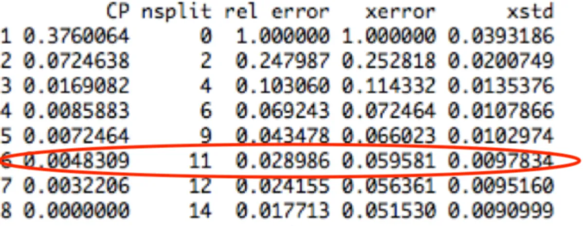
In general, big trees result in overfitting. Therefore, we grow a big tree and prune it back based on the cost-complexity method. We use a rule of thumb to determine the tree size: choose the smallest tree with an “xerror” less than the minimum “xerror” plus its “xstd” [5, 14, 3]. The terminology related to the decision tree method is explained in the next section.

3.3.1 Decision Tree Algorithm

Recursive partitioning is a greedy process because at each step of the tree-building process, the best split is made at that particular step, rather than looking ahead and picking a split that will lead to a better tree in some future step. This process receives a good prediction result on a training data set, but most likely it overfits data, i.e., the prediction result on a test data set may be poor. Therefore, the best way is to grow a very large tree and prune it back based on the cost-complexity method. Cost-complexity is also known as the weakest link pruning.

The authors in [2] considered a sequence of trees given by a nonnegative tuning parameterα instead of considering every possible subtree. They set

up a criterionC(T) such as misclassification rate, Gini index or entropy for each treeT, and computeC(T). The pruning criterion is written as

minC(T) +α|T|, (3.7)

where|T|is the tree size and a large value ofαpenalizes a big tree and tends

(59)

Algorithm of Building a Decision Tree

1. Use recursive binary splitting to grow a large tree on training data, until each terminal node has fewer than some minimum number of observa-tions.

2. Apply the cost complexity pruning to a large tree in order to obtain a sequence of best subtrees, as a function ofα.

3. Use theK-fold cross-validation to chooseα. That is, divide the training

observations intoKfolds. For eachk =1, ...,K:

• Repeat Steps 1 and 2 on all but thekth fold of the training data. • Evaluate the mean squared prediction error on the data in the

left-outkth fold, as a function ofα.

• Average the results for each value ofα, and choose the value of α

which minimizes the average error.

4. Regenerate a tree based on the chosen value ofα.

FIGURE 3.4: Example of How to Determine the Proper Tree Size.

Figure3.4 is an example of the output from Decision Trees. Some terms are explained below.

(60)

3.4. Application of Methodology 37 • CP is the smallest value of the complexity parameterαused in formula

(3.7) that produces a tree with a given number of nodes. • “nsplit” is T−1, whereT is the number of terminal nodes.

• “rel.error” is the residual sum of squares (RSS) with terminal node t

divided by the residual sum of squares with terminal node 1, which is

RSS(t)/RSS(1).

• “xerror” is a 10-fold cross-validated estimate of the error rate for each cost-complexity parameterαlisted.

• “xstd” is the standard deviation between 10 subsample estimates. We use DT because it is easy to understand and easy to interpret results. Peo-ple think that DT mimics the way how peoPeo-ple make decisions. Another rea-son is that trees can handle qualitative predictors without creating dummy variables. One disadvantage of DT is that it generally does not have the same accuracy of prediction as some other regression and classification approaches [7].

3.4 Application of Methodology

In Sections 3.1 to 3.3, we introduced all methods we use in this thesis. In the current section, we discuss how to apply all these methods to predict credit ratings.

For each company, we apply DTW on the ready-to -use set and then use the PCA on the similarity matrix calculated from DTW, then we select the first 20 principal components combined with the long-term credit ratings to form a new data set. The process is outlined in Table3.1. We then employ DT to

(61)

build a prediction model.

DTW Calculate the similarity matrix from clean data set

PCA

Extract important in-formation form matrix

First 20 PCs

Input variables

DT Build a prediction Model

Company

Input Variable

Response Variable

Company 1

PC 1, PC 2, PC 3, ..., PC 20

Credit Rating

Company 2

PC 1, PC 2, PC 3, ..., PC 20

Credit Rating

Company 3

PC 1, PC 2, PC 3, ..., PC 20

Credit Rating

...

Company 52

PC 1, PC 2, PC 3, ..., PC 20

Credit Rating

(62)

39

Chapter 4

Experiments and Results

In this Chapter, we will introduce the results obtained by using different ex-periments and strategies that were described in Chapter2. Sections4.1 and

4.2 entail the comparisons of Common Variables Method vs All Variables Method and different scaling methods for data in 10 grades and 4 grades. Section 4.3 covers the results of Overlapping Method and Section 4.4 sum-marizes the results of sample size increase strategies. Section4.6 gives the details on the examination of the delay effect in credit ratings and the differ-ent splitting affecting credit ratings.

4.1 Common Variables vs All Variables Methods

For each company, there are more than 300 variables available. We assume that all the variables are useful to predict credit ratings. We propose two approaches: one is called Common Variables Method (CV method) and the other one is called All Variables Method (AV method). Our first approach is to use variables that appear among all 52 companies. We extract the common variables first and then employ the methodologies introduced in Chapter3. We use theintersectfunction built-inRto find all the common variables. The second approach is to use all the variables from every company. Here we choose the transformation _stdx−₍X_X¯₎ as a variable scaling method. We use all 10-year financial information and the credit ratings of 2017. Then we compare

(63)

the results produced by the CV and AV methods.

4.1.1 Results for Data with 10 Grades

The results for the CV method of the data with 10 credit rating grades are presented in Table4.1. In Table4.1, the calculation of the training error and the test error is based on the criterion introduced in Section2.6. Column To-tal 0 counts the number of accurately predicted credit ratings. Column ToTo-tal 1 counts the number of predicted credit ratings that have a one-grade dif-ference with true credit ratings. Numbers belonging to the Total 0 column indicate for each test how many predicted credit ratings are the same as the true credit ratings. Numbers belonging to the Total 1 column indicate for each test how many predicted credit ratings are one grade away from the true credit ratings.

TABLE4.1: Common Variables with 10 Grades

Training Error Test Error

Total Total 0 Total 1 Total Total 0 Total 1

Test 1 75 20 5 37 1 0 Test 2 77 20 6 34 1 1 Test 3 91 11 7 25 2 2 Test 4 45 24 6 29 0 3 Test 5 80 18 2 26 1 2 Average 73.6 18.6 5.2 30.2 1 1.6

Ave per Company 1.752 0.44 0.12 3.02 0.1 0.16

The average per company of training error is 1.752, which means that the average distance between the true and the predicted credit ratings is close to 2, i.e., it is a two-grade difference. The average per company of test error is 3.02 which means that the distance between the true and the predicted credit ratings is 3, i.e., it is a three-grade difference. The average training error Total 0 (18.6) and Total 1 (5.2) indicate that in the training data there are almost 19 companies for which the predicted result is the same as the true credit rating

(64)

4.1. Common Variables vs All Variables Methods 41 and there are 5 companies for which the predicted credit rating has a one-grade difference with the true credit rating. The average test error Total 0 (1) and Total 1 (1.6) indicate for the test data there is only 1 company for which the predicted credit rating is the same as the true credit rating, and there are close to 2 companies for which the predicted credit rating has a one-grade difference with the true credit rating.

Secondly, we consider the scenario where we use all the variables collected for each company. The scaling method chosen is _stdx−₍X_X¯₎. The 10-year finan-cial information is used in this analysis. The result for all variables with 10 grades is presented in Table4.2. The average per company of training error is 1.72, which means that the average distance between the true and the pre-dicted credit rating is close to 2, i.e., a two-grade difference. The average per company of test error is 2.08, which means that the distance between the true and the predicted credit rating is 2, i.e., a two-grade difference. The aver-age training error Total 0 (18.8) and averaver-age Total 1 (6) indicate that for the training data there are about 19 companies for which the predicted result is the same as the true credit rating and there are 6 companies for which the predicted credit rating has a one-grade difference with the true credit rating. The average test error Total 0 (1.6) and test error Total 1 (3.4) indicate that for the test data there are data close to 2 companies for which the predicted credit rating is the same as the true credit rating and there are 3 companies for which the predicted credit rating has a one-grade difference with the true credit rating.

Comparing Tables4.1and4.2, we can infer that there is no obvious difference between the CV method and the AV method in terms of the average training errors. The average training error for the AV method is slightly better than that for the CV method. Comparing training Total 0 and Total 1 errors for

(65)

TABLE4.2: All Variables with 10 Grades

Test 1 79 19 5 26 2 2 Test 2 88 11 8 9 4 3 Test 3 54 24 4 27 0 5 Test 4 77 17 8 19 1 4 Test 5 64 23 5 23 1 3 Average 72.4 18.8 6 20.8 1.6 3.4

Ave per Company 1.724 0.45 0.14 2.08 0.16 0.34

both methods, we observe a slight improvement for the AV method. The AV method improves the prediction result by changing the test error from a three-grade difference to a two-grade difference. Test errors Total 0 (1.6) and test error Total 1 (3.4) for the AV method being compared with test error Total 0 (1) and Total 1 (1.6) for the CV method demonstrate a significant improve-ment.

The conclusion from Tables4.1 and4.2 is that the AV method demonstrates a better performance than the CV method for data with 10 categories.

4.1.2 Results for Data with 4 Grades

As mentioned earlier, we can group data with 10 categories into data with 4 categories. We use the same scaling method with _stdx−₍_XX¯₎ and the same methodology with 10-year financial information. The results of the CV method for data with 4 categories are shown in Table4.3. Total 1 in Table4.3 is not the same as in Table4.1with 10 categories. Total 1 in 4 categories only stands for difference between groupsAbandAaa. The reason is thatAbis formed by

Aa1, Aa2, Aa3. If a company’s true credit rating is one ofAa1, Aa2, Aa3and the predicted credit rating of that company isAaathen the error betweenAaa

(66)

4.1. Common Variables vs All Variables Methods 43

TABLE4.3: Common Variables with 4 Grades

Test 1 65 28 0 11 8 0 Test 2 77 24 2 20 6 0 Test 3 83 22 0 11 6 1 Test 4 53 29 2 5 9 0 Test 5 77 27 0 20 1 0 Average 71 26 0.8 13.4 6 0.2

Ave per Company 1.690 0.62 0.02 1.34 0.6 0.02

If a company’s true credit rating isAa3belonging to groupAb, and the pre-dicted credit rating is A1 belonging to group Ac, then the group distance between ratings is 3 but the real distance based on 10 grades is 1. However, if a company’s true credit rating isAa1belonging to groupAb, the predicted credit rating isA3, then the group distance is 3 and the real distance based on 10 grades is 5. If we use a group distance representing the former situation, the result is acceptable. If we use a group distance representing the latter situation, the result is not acceptable because the group experimental error is less than the real error. In the real world we do not know which situation may happen so if the second case occurs it will mislead investors. If investors invest a company, the company’s credit rating belonging toAa1but they treat it asA3company. This misleading would influence the profit. Therefore, we do not consider the difference betweenAbandAcand betweenAcandBaas a one-grade difference.

In Table4.3, the training error average per company is 1.69. It is less than 3, which is the average group assigned value for 4 grades. It means the credit rating can be accurately predicted. The test error average per company is 1.32, which indicates that credit rating prediction is accurate. The average training error Total 0 (26) and average training error Total 1 (0.8) indicate that for the training data there are close to 26 companies for which the predicted

(67)

result is the same as the true credit rating and there is close to 1 company for which the predicted credit rating has a one-grade difference with the true credit rating. The average test error Total 0 (6) and test error Total 1 (0.2) indicate that for the test data there are 6 companies for which the predicted credit rating is the same as the true credit rating and there are no company for which the predicted credit rating is one-grade away from the true credit rating.

The result for the AV method with 4 grades is shown in Table4.4. The aver-age per company of training error is 1.105, which indicates that credit rating prediction is accurate. The test error average per company is 1.32, which indicates that credit rating prediction is accurate. The training error Total 0 (24.2) and the training Total 1 (1.4) indicate that for almost 24 companies in the training data set whose predicted results are the same as the true credit ratings and for one company the predicted credit rating is one grade away from the true credit rating. The test error Total 0 (5.8) and test error Total 1 (0.4) indicate that for almost 6 companies in the test data set whose predicted group credit ratings are the same as the true group credit ratings and for 0 company the predicted credit rating is one grade away from the true credit rating.

TABLE4.4: All Variables with 4 Categories

Test 1 30 28 0 9 8 0 Test 2 49 24 2 11 6 0 Test 3 44 28 2 27 3 1 Test 4 44 30 2 11 7 1 Test 5 65 11 1 8 5 0 Average 46.4 24.2 1.4 13.2 5.8 0.4

(68)

4.2. Using Different Scaling Methods 45 Comparing Tables 4.4 and 4.3, it can be inferred that the AV method gives better results in terms of the average training error, training error Total 1, the average test error and test error Total 1. The CV method gets slightly better results than the AV method in terms of training error Total 0 and test error Total 0.

Comparing Tables4.2and4.4, we observe that better results can be obtained using 4 grades than 10 grades. The same conclusion we can get from Tables

4.1 and 4.3. We can conclude that using all variables can give more accu-rate results than using only common variables. Therefor, we decide to use all variables in the remaining experiments.

4.2 Using Different Scaling Methods

4.2.1 Tests with 10 Grades

We noticed that variables have different magnitudes. Therefore, we proposed several scaling methods in order to seek the method that produces the best results. In this section, we use 5-year financial information starting from 2013 to 2017. 10 years is a relative long time period for a company. We focus on the 2017 credit rating so we think that the last 5 years of financial information is sufficient to compare different scaling methods and also save computational time.

Results for data without scaling with 10 grades is presented in Table4.5. The training error average per company is 1.752, which means that the average distance between the true and the predicted credit ratings is close to 2, i.e., it is a two-grade difference. The test error average per company is 2.28, which means that the distance between the true and the predicted credit ratings is

Predicting Credit Ratings with Statistical Learning Methods

Predicting Credit Ratings with Statistical Learning Methods

Predicting Credit Ratings with Statistical Learning Methods

W

ILFRID

L

AURIER

U

NIVERSITY

M

ASTER

T

HESIS

Predicting Credit Ratings with

Statistical Learning Methods

Author:

Yinduo M

Supervisor:

Dr. Roman M

Dr. Xu (Sunny) W

A thesis submitted in fulfillment of the requirements

for the degree of Master of Science

in the

Department of Mathematics

October 4, 2018

c

Declaration of Authorship

Abstract

Acknowledgements

Contents

List of Figures

List of Tables

List of Abbreviations

Chapter 1

Introduction

1.1

Corporate Credit Ratings

1.2

Moody’s Investors Service Credit Rating

1.3

Literature Review

1.4

Data

1.5

Methodology

1.6

Thesis Structure

Chapter 2

High-dimensional Time Series

Financial Data

2.1

Structure of Data

2.1.1

Data Cleaning

2.2

Data Regrouping

2.3

Comparison Strategies

2.3.1

Common Variables vs All variables

2.3.2

Scaling Methods

2.3.3

10-year Financial Information vs 5-year Financial

Infor-mation

2.4

Strategies of Improving Prediction Accuracy

2.4.1

Examination of Credit Rating Delay Effect

2.5

Training and Test Sets

2.6

Model Evaluation Criterion

2.6.1

Ten Grades

2.6.2

Four Grades

Chapter 3

Methodology

3.1