Neural Network-Based High-Accuracy Motion Control of a Class of Torque-Controlled Motor Servo Systems with Input Saturation

0 INTRODUCTION

The torque-controlled motor servo system has been widely used in the industrial applications in recent years due to its low pollution and high efficiency

compared with its hydraulic counterpart [1]. How to

design a high-performance controller for the motor servo system has been a topic of great interesting in

domestic and foreign research fields [2]. Adaptive

control of nonlinear systems has received much attention for obtaining the global asymptotical stability

of the closed-loop system [3]. However, all kinds of

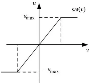
uncertainties always exist in the system, and these uncertainties could deteriorate the systematic control performance severely [4]. Input saturation is one such uncertainty in the motor servo system, and the typical input saturation is shown in Fig. 1. When the input of the actuator reaches a certain limit value, the output of the actuator does not increase with the increase of the input, which is defined as input saturation. Input saturation can deteriorate the dynamic performance and even result in the instability of the system [5].

To deal with the input saturation, one approach is to introduce an additional system to analyse the effect of it. The states of the auxiliary system are employed for controller design and stability analysis

[6]. In [7], an auxiliary design system is introduced

to analyse the input saturation effect. In [8], in order to overcome the problem of input saturation, a new

auxiliary design system and Nussbaum gain functions are incorporated into the control scheme. The control performance could be improved by establishing this kind of auxiliary system, but the model of the system becomes complex, which makes it difficult to be used in engineering applications. A second approach simply takes the input saturation as a kind of disturbance, and an observer is designed for it. An RBF neural network disturbance observer [9], a sliding-mode observer [10] and fuzzy state observer [11] are developed to estimate

Neural Network-Based High-Accuracy Motion Control

of a Class of Torque-Controlled Motor Servo Systems

with Input Saturation

Lei Liu – Jian Hu* _{– Yuangang Wang – Zhiwei Xie}

Nanjing University of Science & Technology, School of Mechanical Engineering, China

The torque-controlled motor servo system is widely used in many industrial applications. However, input saturation often occurs due to the limitation of the actuator output ability, which may worsen the system control performance. In this paper, in order to inhibit the impact of input saturation on the system, a single-hidden-layer neural network based observer is designed to estimate the value of input saturation, which could later be compensated in the proposed controller. In addition, an adaptive law is introduced to estimate the unknown parameters, and a nonlinear robust term is designed to overcome the time-varying disturbances and other compensation errors. The Lyapunov theorem is used to prove the stability of the proposed controller with the neural network-based observer. Extensive comparative experimental results are obtained to verify the high-performance of the proposed control strategy.

Keywords: torque-controlled motor, input saturation, adaptive robust control, neural network, disturbance

Highlights

• Input saturation has been considered when establishing the model of motor servo system.

• Both the parametric uncertainty and the external disturbance have been considered when designing the controller. • A single-hidden-layer neural network has been adopted to estimate the input saturation, which cannot be measured. • Experimental results show the effectiveness of the proposed control strategy.

the unknown disturbance, and the estimation error converges to a compact set if the observer’s parameters are selected appropriately. In [12], the effects of the control singularity and unknown input saturation along with the external disturbance are approximated by a disturbance observer. In [13], fuzzy logic systems are used to approximate the unknown nonlinear functions. Then, the disturbance including the input saturation could be observed and compensated in the controller. Thus, a better tracking accuracy could be obtained and the stability of the system could be guaranteed. However, when the external disturbance is large while the input saturation is relatively small, it is very difficult to eliminate the effect caused by input saturation with the disturbance compensation term.

Another approach involves the establishment of a smooth function to approximate the input saturation nonlinear characteristics [14] to [16]. In

[14], a dynamic signal and smooth function in a

non-affine structure subject to the control input signal are introduced to handle the un-modelled dynamics

and input saturation. In [15], the input saturation is

approximated by a smooth function, and a fuzzy state observer is designed for estimating the unmeasured

states. In [16], a smooth nonlinear function of the

control input signal is first introduced to approximate the saturation function to overcome the effect of non-differential saturation nonlinearity. This method restricted the input saturation nonlinearity, but the authenticity of the system is lost. There are still some other ways to deal with the effects of input saturation. For example, the non-affine problem of input saturation is solved by a mean value theorem

in [17]. A new adaptive sliding mode control scheme

is proposed to guarantee the globally asymptotic convergence of a motion system despite the presence of control input constraint, parametric uncertainties,

and external disturbances in [18]. This method could

directly overcome the impact of input saturation on the system by adjusting the controller’s parameters, but the tracking performance is not sufficient. A single controller is introduced in [19] to constrain the influence caused by input saturation. It can obtain better tracking accuracy, but the robustness of the system simultaneously decreased.

According to the above analysis, all the proposed controllers have both advantages and disadvantages. In this paper, an adaptive robust control method is proposed to improve the tracking accuracy of motion systems driven by torque-controlled motors with input saturation. Considering the universal approximation ability of neural networks (NN) [20] and [21], a kind

of single-hidden layer parameter linearized NN [22]is

designed to approximate the input saturation, and the input saturation is compensated effectively later in the controller. The experiment results verify the validity of the proposed controller. This method considers both the input saturation and the disturbance in the system, therefore, it has better performance than the other controllers do.

This paper is organized as follows. The dynamics of a motor servo system are established in Section 2. Section 3 designs an adaptive robust controller with a NN-based observer in detail. A Lyapunov stability proof and analysis has also been given in this part. Extensive experiments are carried out in Section 4, and the conclusions are given in Section 5.

1 DYNAMICS OF A TORQUE-CONTROLLED MOTOR SERVO SYSTEM

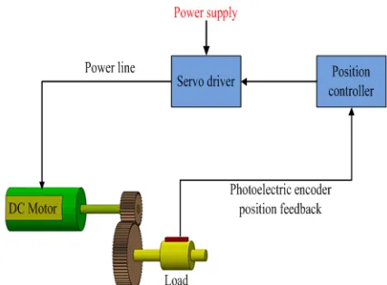
In this part, an accurate model of a torque-controlled motor servo system is established. A torque-controlled motor servo system is usually composed of a torque-controlled motor, a servo driver, a position controller,

a reducer, sensors, and so on [23] and [24]. The

systematic diagram is shown in Fig. 2.

Fig. 2. Specific composition diagram of the motor servo system

response speed is much higher than the mechanical response speed. Considering all the above factors

[25] and [26], the mathematic model of the

torque-controlled motor servo system can be described as:

J y k u Bequ= ⋅ −u equ⋅ −y d n−f t( ), (1)

where Jequis the equivalent inertia of the motor and

load, y is the position of the load, ku is the

voltage-torque coefficient, u is the control input, Bequ is

the equivalent viscous friction coefficient, dn is

the constant disturbance, f(t) is the time-varying

disturbance.

Before the controller is designed, some hypotheses should be made as follows:

1) All the parameters of system are invariant variables or slowly time-varying variables. That is Jequ =ku =Bequ =dn =0.

2) All the parameters are bounded, and the upper/ lower bounds for all these parameters are known. Assuming that the input saturation exists in the

actuator. u is the output of the actuator, the maximum

value of u is umax, v is the control input of the actuator,

δ is the input saturation. u = δ + v, u = sat(v), the function sat(v) can be expressed as:

sat v

u v u

v v u

u v u

( ) , , | | , max max max max max = > ≤ − <      , (2)

It is necessary to build a state space equation of the system for designing a controller for the system. Thus, a number of parameters are defined: θ1= Jequ / ku,

θ2=Bequ/ku, θ3=dn/ku. Then, the mathematical

model, Eq. (1), can be rewritten as:

θ1y v= −θ2y− −θ τ3 ( )t +δ, (3) where τ(t) = f(t) / ku indicates the time-varying

disturbance and other systematic un-modelled nonlinearities.

Denote the state variables as:

x y x y 1 2 = =  

 . (4)

Then the state space equation of the system could be obtained as follows:



 

x x

x v y t

1 2

1 2 2 3

=

= − − − +

 

θ θ θ τ( ) δ. (5)

2 DESIGN OF A CONTROLLER WITH NEURAL NETWORK BASED OBSEVER

2.1 Neural Network Based Observer Design

In the mechanical-electrical servo system, the state of the system is nonlinear, time-varying, and uncertain; in other words, it is very difficult to know the precise value of overflow by using the sensor and other measuring tools. Designing an observer to observe the overflow of input saturation is necessary. A NN can approximate any smooth nonlinear function to within arbitrary accuracy when given a sufficient number of hidden layer neurons and input information. Thus, a single hidden-layer network is defined to approximate the unknown parameter δ.

The mathematical expression of the single-layer NN is as follows:

δ =W h xT +ε

approx

* _{( )}

, (6)

h x c

b

j j

j

=exp(−|| − || ), 2

2 2 (7)

where x = [x1x2 ...xn]T is the input of network, j is the jth _{node of the hidden layer, h = [hj]}T _{is the output of}

network’s Gauss radial function, cj = [cj1cj2 ...cjn] is

centre vector value of the jth _{node, b = [b1 b2 ...bm]}T

is the width of the Gauss basis function, W*T _{is ideal}

weights of NN,

ε

NN and

ε

≤ ε

.

The input of the neural network is chosen as

x = [x1, x2]T_{, and then the real output of the network is:} δ=W h xT ( ), (8)

where W represent the estimated value of W*_{. Design}

the adaptive law of weights as follows:

(9) where Proj and and otherwis W i W i W i i W W i _i i _i    ( ) , , , max min ⋅ =

= ⋅ >

= ⋅ <

⋅ 0 0 0 0 ee      

, (10)

and Γ2 is the adaptive law matrix of weights.

Define W W W= − *_{, thus}

δ δ ε ε ε − = + − = − + = − +

 _{W h x W h x}

W W h x W h x

T approx T T T approx T * * ( ) ( ) ( ) ( )

Remark 1: Input saturation is an inevitable phenomenon in mechanical-electrical servo systems, so the impact of the input saturation should be restrained when designing the controller. How to compensate the overflow of input saturation is the key to solving the nonlinear problem. A single hidden-layer network-based observer can estimate the overflow δ and the estimation error of the single hidden-layer network can be close to 0 as long as the nodes in the hidden layer are enough in theory. That is to say, the single hidden-layer network can approximate δ within arbitrary accuracy. It is obvious that the value of δ could be replaced by estimation

value δ when designing the controller later, and the

control performance could be observably improved.

2.2 Design of a Controller

The system that is driven by a torque-controlled motor is a typical motor servo system, and the control system is a second-order system. The design process of a specific controller is as follows.

Step 1. In this step, x2 is deemed a dummy control input. And x2 is regarded as the dummy control input; afterwards, a control function x2eq ought to be

designed for x2. The result in the tracking property

is guaranteed. Denoting x1d as the ideal position and z1 = x2 – x1d indicate the position tracking error. After

that, the dynamic equation of error is as follows:

   

z1= −x x x x1 1_d= 2− 1_d. (12) Let z2 = x2 – x2eq indicates the error between the

virtual input and the real input, thus the Eq. (12) can be rearranged as follows:

 

z1=z2+x2eq−x1d. (13)

Based on Eq. (13), the resulting virtual control law x2eq could be designed as follows:

x2_eq =x1_d −k z1 1, (14)

where k1 > 0. Substituting Eq. (14) into Eq. (13), we could obtain:



z1=z k z2− 1 1. (15) From Eq. (15), it is indicated that we want to turn

z2 converge into zero to turn z1 converge into zero.

Step 2. The dummy control law x2eq has been

designed in Step 1. In this step, we need to design the real control law for v. The time derivative of z2 can be given by:

θ θ θ

θ θ τ δ θ

1 2 1 2 1 2

2 2 3 1 2

  



z x x

v x t x

v eq eq = − = − − − + − = ( )

−−θ1 2x eq−θ2 2x − −θ τ3 ( )t +δ. (16)

To make z2 converge to 0, the following control

law v is proposed:

v v v= +_{a s}, (17)

v_a=θ_{1 2}x _eq+θ_{2 2}x +θ₃−δ_{, (18)}

v vs= s1+vs2, (19)

v_s k z v_s h zs s

1 2 2 2

2

2 4

= − , = − ,

ε (20)

where va is the feed-forward compensation term of

the system model, vs1 is a linear robust feedback term

to stabilize the system nominal model and k2 > 0, vs2

is a nonlinear robust feedback term which is used to compensate for the time-varying disturbance and the model error.

Substituting Eqs. (18) and (11) into Eq. (16), later the Eq. (16) could be transformed to:

θ θ θ θ δ δ τ

θ

1 2 1 2 2 2 3 2 2 2

1 2

z x x k z v t

x eq s eq = + + − + − + − = ( ) ++ + − − + + − = − − − − θ θ ε τ θ

2 2 3 2 2

2

2 2 1

x k z

W h x v t

x x T s T eq ( ) ( ) _ _ − − − + − + − − = + + v

W h x k z t

v W h x k z s T T s T 2 2 2 2 2 ( ) ( ) ( ) ε τ θ ϕ ε

₂₂−τ( ),t (21)

where θ1, θ2, θ3 is unknown, and the value would be

changed in the working process of the system, in order to design the controller simply, we should adopt the estimated value to replace the uncharted parameter when designing the controller, (for example θ1, θ2, θ3). Thus, a parameter matrix θ = [θ1 θ2 θ3] and an

estimated parameter matrix θ=θ1 θ2 θ3 should

be defined. Based on Assumption 2.1, we could obtain:

θ∈Ω_θ =

{

}

|τ(t)|<δ_d, (23)

where θ_min =

[

]

θ_max=

[

]

the upper and lower bounds are known, and δdis a

Step 3. In this step, an estimator should be designed to estimate the unknown system parameters. In order to make both the estimated parameters and the model uncertainty bounded, design a discontinuous projection gradient type parameter adaptation law as follows:

(24) where

Proj

and and otherwis θ

θ θ

θ θ



 

( ) , , ,

max

min

⋅ =

= ⋅ >

= ⋅ <

⋅

i

i i i

i _i

i _i

0 0

0 0

ee 

 

  

, (25)

ϕ = − − −

 x eq x 

T

2 2 1 . (26)

φ is the parameter adaptive regression, Γ1 is

the adaptation law matrix, in addition, there are the following properties:

θ∈L_∞, θ_Proj_θ(Γϕz₂)−Γϕz_2≤0, (27)

where

θ θ θ

= -

estimation.

Step 4. In this step, in order to overcome the parameters approximation error and approximation error of model uncertainty, a nonlinear robust feedback item us2 should be designed to stabilize the

system and improve the tracking performance.

Define v_s2 h zs s

2

2 4

=(− ) ε , where this represents

all the errors’ upper bound, and it means

|θ φT | |+ W h xT ( ) | | |+ ε δ+ _d≤h_s, εs is a positive

real number which has the following characters:

i z v W h x t

ii z v

s T T S

s

: ( ) ( )

:

.

2 2

2 2 0

− − − −

  ≤

⋅ ≤

   

 

θ ϕ ε τ ε

(28)

2.3 Stability Analysis

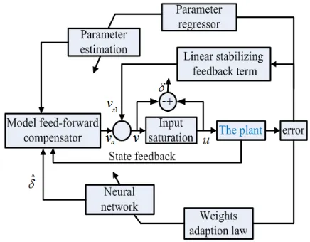
The specific diagram of control tactics is shown in Fig. 3. The strategy adopts an NN observer to estimate the state that cannot be measured, and the weight adaptive velocity is used to estimate the weights online. In addition, the parameter regression is used to estimate the unknown parameters; all the estimated parameters are required in the feed-forward compensator. A linear

robust term vs1 is designed to overcome the constant

disturbance of the system, and a nonlinear robust

term vs2 is designed to compensate the time-varying

disturbance and modelling errors.

Fig. 3. The neural network observer based robust adaptive control tactics graph

Based on the controller designed earlier, we could obtain the following theorem:

Theorem 2.1. With the NN-based observer, Eqs. (8) and (9), the parameter adaption law in Eq. (24), the adaptive robust full state feedback control law in Eq. (17), we can obtain a specified transient and everlasting performance in the sense that limiting the tracking error to a small extent by a known function exponentially converges to the

( ) ( ) (

)

Proof: See Appendix 7.1.

Remark 2: The consequence of theorem 2.1 denotes that the contrivable controller consists of a robust adaptive controller and NN-based observer, which has an exponential convergence transitory property with the exponentially converging rate λ, and the ultima tracking error was inhibited by adjusting the system’s parameters online. The parameter adaption law could approximate the unknown system parameters, and the weight adaptive law could estimate the value of the weights. The constant disturbance of the system was compensated by the feed-forward compensation item which used the estimated parameters. Moreover, the input saturation was compensated by the output value of the NN based observer. Furthermore, the nonlinear robust feedback item was proposed to reduce the effect of parameter estimation error and weights estimation error, which could effectively improve the stability of the closed-loop system.

full state feedback control law, Eq. (17), the system could achieve asymptotic export tracking merely in the presence of parametric uncertainty.

Proof: See Appendix 7.2.

Remark 3: The consequence of theorem 2.2 denote that the adaptive robust controller based on an NN observer could obtain improved tracking performance, and the system could achieve asymptotic export tracking in the absence of the estimated error of NN.

3 EXPERIMENTAL RESULTS

The experimental platform of torque-controlled motor servo system is shown in Fig. 4. This experimental platform consists of a torque-controlled servomotor, a speed reducer, a slewing mechanism, a photoelectric encoder, sensors, a power supply, and an IPC. The photoelectric encoder could sample the position signals of the two servo-motor. The voltage signal is transmitted to the driver by using a (digital/analogue) D/A board card.

Fig. 4. The experimental platform of torque-controlled motor servo system

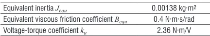
The parameters of the experimental platform are given as follows:

Table 1. The parameters used in experiment

Equivalent inertia Jequ 0.00138 kg·m2 Equivalent viscous friction coefficient Bequ 0.4 N·m·s/rad Voltage-torque coefficient ku 2.36 N·m/V

Three controllers are compared for a sinusoidal-like motion trajectory, and two cases are compared for this normal motion trajectory. Case 1 is “constant disturbance case”: Setting the constant disturbance

as dn = 0.5. Then, after a simple calculation, we can

obtain: θ1 = 0.01, θ2 = 0.294, θ3 = 0.36. Case 2 is

“time-varying disturbance case”: The time-varying

disturbance in the system was set as f(t) = 0.015∙x1∙x2,

and x1, x2 are state variables selected. The three

controllers are as follows:

1) The proportional–integral–derivative controller (PID): in industrial control applications, the PID controller was used widely, its proportional integral differential control of position and speed loop has low dependence on the system model, and could obtain a high accuracy. In this experiment, the PID controller of position loop is used, and its three parameters could be adjusted by observing the position error. Denote the parameters of the proportional, integral and differential as kp = 25, ki = 0.8, kd = 0.

2) The adaptive robust controller (ARC): in the closed-loop system was realized by the control law, Eq. (17), and the parameter adaptive law, Eq. (24), which designed in the above, and the effect caused by input saturation was not considered in this case. In this experiment, the feedback

gains are chosen as k1 = 35, k2 = 002. The

upper and the lower bounds of parameters are θmax = [0.05, 0.5, 0.5], θmin = [0.005, 0.01, 0.01].

3) The adaptive robust controller with neural network based observer (ARCNN): The control gains are chosen as k1 = 20, k2 = 0.01, and [v z2] is the input of the NN, the parameters of the Gauss basis function was designed via the actual input extent of the network; therefore, choose

cj = 8 × [–1, –0.5, 0, 0.5, 1], bj = 5, in this case,

and define the initial value of network weights as zero.

In order to verify the feasibility of the adaptive robust controller based on the NN observer, set the limitation of input saturation in actuator:

umax = 0.45, umin = –0.45. The desired output signal: yd = x1(t) = 2 ×sin(3.14t)[1 – exp(–0.01t)] [°]. To ensure

that the performance of the designed controller is fully demonstrated, the sample time at least is set to 15 s.

Table 2. The accuracy of the three controllers in Case 1: “constant disturbance case”

Controller Time [s] Accuracy [°]

ARC t > 5 0.062

PID t > 5 0.045

ARCNN t > 10 0.0028

ARC controller in terms of both transient and final tracking errors, the result of experimental indicate that the impact caused by input saturation could not be ignored in the control system. By comparing the control performance of the three controllers, the ARCNN controller has the best tracking property, and its maximum steady tracking error is about 0.0028°. Fig. 6 shows the voltage signals v and u; v

is the voltage signal before the saturation constraint

occurred, and u is the voltage signal after the

saturation constraint occurred; from the picture we can see the error between v and u cannot be ignored, thus the effect of input saturation should be considered. Fig. 7 shows the overflow of input saturation and corresponding estimation. It can be seen that the NN observer could estimate the overflow immediately and thus the input saturation could be compensated effectively. In addition, ARCNN adopts the parameter adaptive law and the weights adaptive law to estimate uncertain parameters and weights, which are used in the feed-forward compensation item. Therefore, a high performance was realized, which also proved the validity of the adaptive control law.

Fig. 5. Tracking error of three controllers in Case 1

Fig. 6. The voltage signal v, u in Case 1

Fig. 7. The true value and the estimated value of input saturation in Case 1

Table 3. The accuracy of the three controllers in Case 2: “time-varying disturbance case”

Controller Time [s] Accuracy [°]

ARC _t > 5 0.056

PID _t > 5 0.045

ARCNN t > 5 0.035

The position curve in the ideal state and the homologous tracking property of the three controllers in Case 2 is revealed in Fig. 8. As seen from the figure, the input saturation is compensated by NN or PID has the better tracking performance than uncompensated, which confirms that the accuracy of the estimation is very important. Fig. 9 indicate that the voltage before and after saturation constrain, as seen when t ≤ 1 s, the

less than 0.0035°; this also proved the effectiveness of parameter adaptive estimation and NN weight estimation in the presence of constant disturbance and time-varying interference (adaptive parameter estimation curve is shown in Fig. 11).

Fig. 11. Adaptive parameter estimation curve of ARCNN in Case 2

4 CONCLUSIONS

In this paper, considering the universal approximation ability of NN, a single hidden-layer NN based observer is designed to estimate the input saturation of the system, which is later compensated in the controller. An adaptive law is introduced to estimate the unknown parameters, and a nonlinear robust term is designed to overcome the time-varying disturbances. The NN weight adaption law has been deduced by using the Lyapunov method. The proposed controller pledges the asymptotic stability of the tracking performance under the condition that the NN estimation error is zero. The effectiveness of the proposed control strategy has been proved by comparing the experimental results. In the future, the input saturation and external disturbance should be estimated by designing a double- observer, which

is helpful in improving the control precision of the

motor servo system.

5 ACKNOWLEDGMENT

This work was supported by the National Natural Science Foundation of China under Grant 51505224, and the Natural Science Foundation of Jiangsu Province in China under Grant BK2015776.

6 REFERENCES

[1] Yao, J., Jiao, Z., Ma, D.. (2014). Adaptive robust control of dc motors with extended state observer. IEEE Transactions

Fig. 8. Tracking error of three controllers in Case 2

Fig. 9. The voltage signal v, u in Case 2

on Industrial Electronics, vol. 61, no. 7, p. 3630-3637,

DOI:10.1109/TIE.2013.2281165.

[2] Chen, M., Ge, S.S., Ren, B. (2011). Adaptive tracking control of uncertain MIMO nonlinear systems with input constraints. Automatica, vol. 47, no. 3, p. 452-465, DOI:10.1016/j. automatica.2011.01.025.

[3] Mesloub, M., Benchouia, M.T., Golea, A. (2017). A comparative experimental study of direct torque control based on adaptive fuzzy logic controller and particle swarm optimization algorithms of a permanent magnet synchronous motor. The International Journal of Advanced Manufacturing Technology, vol. 90, no. 1-4, p. 59-72, DOI:10.1007/s00170-016-9092-4.

[4] Zong, Q., Wang, F., Tian, B. (2014). Robust adaptive dynamic surface control design for a flexible air-breathing hypersonic vehicle with input constraints and uncertainty. Nonlinear Dynamics, vol. 78, no. 1, p. 289-315, DOI:10.1007/s11071-014-1440-z.

[5] Esfandiari, K., Abdollahi, F., Talebi, H. (2015). Adaptive control of uncertain nonaffine nonlinear systems with input saturation using neural networks. IEEE transactions on Neural Networks and Learning Systems, vol. 26, no. 10, p. 2311-2322,

DOI:10.1109/TNNLS.2014.2378991.

[6] Li, Y., Tong, S., Li, T. (2013). Direct adaptive fuzzy back-stepping control of uncertain nonlinear systems in the presence of input saturation. Neural Computing and Applications, vol. 23, no. 5, p. 1207-1216, DOI:10.1007/s00521-012-0993-3.

[7] Gao, S., Dong, H., Ning, B., Chen, L. (2015). Neural adaptive control for uncertain nonlinear system with input saturation: State transformation based output feedback. Neurocomputing, vol. 159, p. 117-125, DOI:10.1016/j. neucom.2015.02.012.

[8] Chen, M., Ge, S. (2013). Direct adaptive neural control for a class of uncertain nonaffine nonlinear systems based on disturbance observer. IEEE Transactions on Cybernetics, vol. 43, no. 4, p. 1213-1225, DOI:10.1109/TSMCB.2012.2226577.

[9] Ammar, A., Bourek, A., Benakcha, A. (2017). Nonlinear SVM-DTC for induction motor drive using input-output feedback linearization and high order sliding mode control. ISA Transactions, vol. 67, p. 428-422, DOI:10.1016/j. isatra.2017.01.010.

[10] Yao, J., Jiao, Z., Ma, D. (2014). RISE-based precision motion control of dc motors with continuous friction compensation. IEEE Transactions on Industrial Electronics, vol. 61, no. 12, p. 7067-7075, DOI:10.1109/TIE.2014.2321344.

[11] Yao, J., Yang, G., Jiao, J., Ma, D. (2013). Adaptive robust motion control of direct-drive DC motors with continuous friction compensation. Abstract & Applied Analysis, vol. 2013, p. 1-14,

DOI:10.1155/2013/837548.

[12] Wang, H., Liu, X., Liu, K. (2015). Adaptive neural data-based compensation control of non-linear systems with dynamic uncertainties and input saturation. IET Control Theory Application, vol. 9, no. 7, p. 1058-1065, DOI:10.1049/iet-cta.2014.0709.

[13] Sui, S., Tong, S. Li, Y. (2014). Predefined performance fuzzy adaptive tracking control for nonlinear stochastic systems with input saturation. International Conference on Mechatronics and Control, DOI:10.1109/ICMC.2014.7231572.

[14] Sun, W., Gao, H., Kaynak, O. (2011). Finite frequency

H∞ control for vehicle active suspension systems. IEEE Transactions on Control Systems Technology, vol. 19, no. 2, p. 416-422, DOI:10.1109/TCST.2010.2042296.

[15] Wang, H, Chen, B. Liu, X., Liu, K., Lin, C. (2014). Adaptive neural tracking control for stochastic nonlinear strict-feedback systems with unknown input saturation. Information Sciences, vol. 269, p. 300-315, DOI:10.1016/j.ins.2013.09.043.

[16] Zhou, Q., Shi, P., Tian, Y., Wang, M. (2015). Approximation-based adaptive tracking control for MIMO nonlinear systems with input saturation. IEEE Transactions on Cybernetics, vol. 45, no. 10, p. 2119-2128, DOI:10.1109/TCYB.2014.2365778.

[17] Wu, J., Liu, K., Han, D. (2013). Adaptive sliding mode control for six-DOF relative motion of spacecraft with input constraint. Acta Astronautica, vol. 87, p. 64-76, DOI:10.1016/j. actaastro.2013.01.015.

[18] Zong, Q., Wang, F., Su, R. (2015). Robust adaptive back-stepping tracking control for a flexible air-breathing hypersonic vehicle subject to input constraint. Institution of Mechanical Engineers, vol. 229, no. 1, p. 10-25,

DOI:10.1177/0954410014525128.

[19] Yao, J., Jiao, Z., Ma, D. (2014). Extended-state-observer-based output feedback nonlinear robust control of hydraulic systems with back-stepping. IEEE Transactions on Industrial Electronics, vol. 61, no. 11, p. 6285-6293, DOI:10.1109/ TIE.2014.2304912.

[20] Uran, S., Šafarič, R. (2012). Neural-Network estimation of the

variable plant for adaptive sliding-mode controller. Strojniški vestnik - Journal of Mechanical Engineering, vol. 58, no. 2, p. 93-101, DOI:10.5545/sv-jme.2011.098.

[21] Zilkova, J., Timko, J., Girovsky, P. (2012). Modelling and control of tinning line entry section using Neural Networks. International Journal of Simulation Modelling, vol. 11, no. 2, p. 97-109, DOI:10.2507/IJSIMM11(2)4.210.

[22] Hu, J., Liu, L., Wang, Y.G., Xie, Z. (2016). Precision motion control of a small launching platform with disturbance compensation using neural networks. International Journal of Adaptive Control and Signal Processing, vol. 31, no. 7, p. 971-984, DOI:10.1002/acs.2743.

[23] Alonge, F., Cirrincione, M., D’lppolito, F., Pucci, M., Sferlazza, A. (2016). Adaptive feedback linearizing control of linear induction motor considering the end-effects. Control Engineering Practice, vol. 55, p.116-126, DOI:10.5545/sv-jme.2011.098.

[24] Hu, J., Qiu, Y., Liu, L. (2016). High-order sliding-mode observer based output feedback adaptive robust control of a launching platform with backstepping. International Journal of Control, vol. 89, no. 10, p. 2029-2039, DOI:10.1080/00207179.2016 .1147604.

[25] Mrčela, T., Žeželj, D., Panić, N. (2009). Linear loading

measurement line for static torque and its performance. Tehnički vjesnik – Technical Gazette, vol. 22, no. 5, p. 1093-1098.

[26] Ahmad, F., Hudha, K., Mazlan, S.A., Jamaluddin, H., Zamzuri, H., Kadir, Z.A., Aparow, V.R. (2017). Modelling and control of a fixed calliper-based electronic wedge brake. Strojniški vestnik - Journal of Mechanical Engineering, vol. 63, no. 3, p. 181-190,

7 APPENDICES

Proof of Theorem 2.1: Without considering the neural network estimation error, the Lyapunov function is established as follows:

v t1 1 2z 2 1 2

( )= θ , (29)

v z z

k z v W h x z

k z

s T T approx

1 1 2 2

2 2 2

2 2

2 2

=

= − + − − −

≤ − θ

θ ϕ ε

( ( ) )

2 2

2 1

1

1 2

+ε = − + ≤ − +

θ ε λ ε

s k V( ) s V s, (30)

where λ=2k2/θ1min , we can obtain:

V t V t s t

1( )≤ 1( ) exp(0 −λ )+ [1−exp(− )].

ε

λ λ (31)

With the passage of time, the position tracking error and angular velocity tracking error will be limited to a certain extent.

| | ,

min

z s s

2

1 1

2 2

= ε ≤

λθ

ε

λθ (32)

| | .

min z

k s

1

1 1

1 2

≤ ε

λθ (33)

Proof of theorem 2.2: when εapprox = 0, consider

the following Lyapunov function candidate:

V Z T W WT

2 1 2

2 1

1

2 1 1

2

1 2

1 2

= _θ + _Γ−_{θ θ} + _Γ−  

, (34)

V z z T W WT

2 1 2 2 1

1

2 1

=_θ +_Γ−_{θ θ}+_Γ−

. (35)

Since θ and W are invariant or slowly varying

variables, we could have . Then we

could obtain: