UC San Diego
UC San Diego Electronic Theses and Dissertations
TitleInformative Hyper-parameter Optimization and Selection Permalink
https://escholarship.org/uc/item/7tj9c69t Author
Yepremyan, Alice Repsimeh Publication Date
2019
UNIVERSITY OF CALIFORNIA SAN DIEGO
Informative Hyper-parameter Optimization and Selection
A Thesis submitted in partial satisfaction of the requirements for the degree
Master of Science in Bioengineering by Alice Yepremyan Committee in charge:
Gert Cauwenberghs, Chair Todd Coleman
Gabriel Silva Brian Wilson
Copyright Alice Yepremyan, 2019
The Thesis of Alice Yepremyan is approved, and it is accept-able in quality and form for publication on microfilm and electronically:
Chair
University of California San Diego
TABLE OF CONTENTS
Signature Page . . . iii
Table of Contents . . . iv
List of Figures . . . vi
List of Tables . . . vii
Acknowledgements . . . viii
Abstract of the Thesis . . . ix
Chapter 1 Introduction . . . 1
1.1 Overview of problems . . . 3
1.2 Significance . . . 3
1.2.1 Existing Research projects . . . 3
1.2.2 Non-Expert Users . . . 5
1.3 Main Thesis Thrust . . . 5
1.4 Thesis Organization . . . 6
Chapter 2 Related Work . . . 7
2.1 AutoML Research . . . 7
2.2 Meta-Learning Applications . . . 8
2.3 Recent Approaches to Analyzing Optimizers . . . 8
Chapter 3 Material and Methods . . . 10
3.1 Experimental Setup . . . 10
3.1.1 Data . . . 10
3.1.2 Preprocessing of data . . . 11
3.1.3 Meta-features . . . 12
3.1.4 Algorithms . . . 13
3.1.5 Hyper-parameter search spaces . . . 14
3.2 Optimization Methods . . . 15 3.2.1 SMAC . . . 15 3.2.2 Hyperopt . . . 16 3.2.3 BOHB . . . 16 3.2.4 Excluded techniques . . . 17 3.2.5 Performance Measure . . . 18 3.3 Automation . . . 18 3.3.1 Analysis setup . . . 18 3.3.2 Auto-ML setup . . . 19 3.3.3 Meta-data . . . 19
3.3.4 Prediction of optimization improvement over defaults . . . . 20
Chapter 4 Results and Discussion . . . 21
4.0.1 Hyper-parameter search space . . . 21
4.0.2 Exploring the selection of categorical values . . . 21
4.0.3 Exploring the selection of extreme continuous values . . . . 22
4.0.4 Effect of tuning and model selection . . . 26
4.0.5 Optimization times . . . 28
4.0.6 Analysis of performance on hard and easy problems . . . . 29
4.0.7 Performance by Dataset . . . 32
4.0.8 Performance by Algorithm . . . 33
4.1 Optimization prediction model . . . 33
Chapter 5 Conclusion . . . 37
Appendix A Hyper-parameters . . . 40
Appendix B Meta-features . . . 46
Appendix C Datasets . . . 50
Appendix D Additional Analysis . . . 54
LIST OF FIGURES
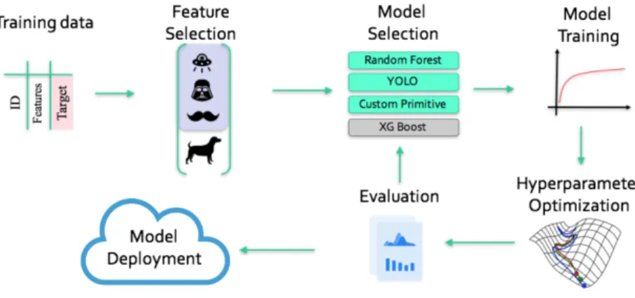
Figure 1.1: Simplified work flow of data driven discovery of complex models in D3M . 4 Figure 3.1: Meta-data of each dataset was transformed into two principal components to
show variance and diversity between each dataset used in this analysis . . . . 11 Figure 3.2: Diagram of optimization plug-in with the auto-composition pipeline
frame-work of D3M . . . 19 Figure 4.1: Evolution of the hyper-parameter ‘kernel’ for SVC on arrhythmia dataset . 23 Figure 4.2: Histogram of counts of max and min continuous values over all datasets . . 24 Figure 4.3: Histogram of counts of continuous values over all datasets . . . 26 Figure 4.4: Bar plot of percent improvement over default values vs. the number of
datasets that achieved that value. BOHB(blue), SMAC(orange), Hyper-opt(green) . . . 27 Figure 4.5: Stacked bar plot of percent improvement over default values vs. the number
of datasets that achieved that value. The colors represent each algorithm evaluated. . . 28 Figure 4.6: Mean rankings of the algorithms across all datasets . . . 36
LIST OF TABLES
Table 4.1: Run times (in seconds) for each optimizer on the arrhythmia dataset correlating to Figure 4.1 . . . 22 Table 4.2: Avg. Time in seconds to beat default loss. . . 29 Table 4.3: BOHB: Performance of most optimal hyper-parameter settings on ‘hard’ and
‘easy’ problems. Values in bold indicate columns which were discussed in section 4.0.6 . . . 31 Table 4.4: Hyperopt: Performance of most optimal hyper-parameter settings on ‘hard’
and ‘easy’ problems. Values in bold indicate columns which were discussed in section 4.0.6 . . . 31 Table 4.5: SMAC: Performance of most optimal hyper-parameter settings on ‘hard’ and
‘easy’ problems. Values in bold indicate columns which were discussed in section 4.0.6 . . . 32 Table 4.6: Raked meta-features for predicting percent optimization for SMAC . . . 34 Table 4.7: Raked meta-features for predicting percent optimization for BOHB . . . 34 Table 4.8: Raked meta-features for predicting percent optimization for Hyperopt . . . 35 Table A.1: Hyper-parameters tuned for each ML algorithm. λrefers to the total number
of hyper-parameters that were tuned. . . 40 Table B.1: Meta-features. 49 meta-features in total. . . 46 Table C.1: Datasets used in experiments from OpenML . . . 50 Table D.1: Hyperopt: The average time, minimum time, and maximum time to beat the
default hyper-parameter settings across all datasets in seconds . . . 54 Table D.2: BOHB: The average time, minimum time, and maximum time to beat the
default hyper-parameter settings across all datasets in seconds . . . 55 Table D.3: SMAC: The average time, minimum time, and maximum time to beat the
ACKNOWLEDGEMENTS
I would first like to express my sincere gratitude to Gert Cauwenberghs and Brian Wilson for their mentorship, motivation, and constructive critiques throughout the process of writing this thesis. I would also like to thank Chris Mattmann, who not only agreed to fund this research but also provided continuous advice and assistance.
I would also like to extend my thanks to the DARPA Data-driven discovery program for their generous funding and for their help in offering me the resources to conduct my research. I am also grateful for my colleagues from my internship at the Jet Propulsion Laboratory for always willing to extend their help and support.
Lastly, I wish to thank my parents, friends, and family for their unfailing support and momentum throughout my research endeavor.
ABSTRACT OF THE THESIS
Informative Hyper-parameter Optimization and Selection
by
Alice Yepremyan
Master of Science in Bioengineering
University of California San Diego, 2019
Gert Cauwenberghs, Chair
Hyper-parameter optimization methods allow efficient and robust hyperparameter search-ing without the need to hand-select each value and combination. Although hyper-parameter tuners, such as BOHB, Hyperopt, and SMAC have been investigated by researchers in terms of performance, there has yet to be an in-depth analysis of the values each tuner selected over all iterations. We propose a thorough aggregation of data in terms of the efficiency of the search values selected by each tuner over 59 datasets and ten popular ML algorithms from Scikit-learn. From this extensive data accumulated, we observe and advise which tuners show better results for particular datasets, through its meta-data, and algorithms. Through this research, we have also developed a simple plug-in for BOHB, Hyperopt, and SMAC into DARPA’s Data-driven discovery
(D3M) Auto-ML systems for smooth implementation of various tuners. This is advantageous as the desired hyper-parameter tuner may change depending on the pipeline search method in an Auto-ML system, particularly when compared with Auto-ML systems that only utilize one search method. Our results show that for Auto-ML systems, the Hyperopt tuner will give more desirable results in a fewer amount of iterations due to the significant exploration component, and BOHB performs the best generally over a large number of datasets and algorithms owing to strategic budgeting.
Chapter 1
Introduction
With the expanding field of data science, there is growing research towards automating model selection and making data science tools more accessible to non-experts. These Auto-ML systems seek to reduce the need for human interaction and increase performance by automatically generating pipelines that link various primitives, or models, together. Many have started using meta-learning, or using knowledge from previous runs, in order to make informative generations of pipelines [6]. For example, Auto-Sklearn utilizes meta-data from previous runs in order to automate pipeline construction and initialize the Bayesian Optimizer [5]. Through meta-learning, Auto-Sklearn has been able to demonstrate significant performance gains with improved searching efficiency.
The optimization of hyper-parameters can also lead to significant performance gains. Hyper-parameters are parameters that cannot be estimated or learned from the data and need to be manually set. Hyper-parameter values can have a considerable impact on the behavior of a model, and the performance of a model can be greatly affected by even small changes in these values [11][12][24]. Many Auto-ML systems rely on only one singular optimization technique, however, there has not yet been a structured analysis on which optimization technique is best suited for Auto-ML purposes.
Classical machine learning (ML) algorithms from the Scikit-learn library have between having two to fourteen hyper-parameters. The search space of hyper-parameter values can increase significantly with the addition of hyper-parameters, especially those which are real-valued. Moreover, some ML algorithms can be more sensitive to hyper-parameter tuning than others [14]. Thus, there is a need to understand how specific optimization techniques search in various situations. In other words, observing how tuners perform with various algorithms, a large number of hyper-parameters, easy or difficult input data, etc.
In this thesis, we explore various popular optimization methods in terms of performance, searching, and run times. We also use this information to estimate the expected optimization upper limit for the given inputs such as meta-data of the dataset, learning algorithm, and hyper-parameter optimization technique. From this, we can extract the feature importance for each tuner, which can potentially influence which optimizer to use under certain meta-data conditions. We envision that people will use this data and research in order to understand better how different optimization techniques search and which methods serve their time and accuracy needs.
Furthermore, we have designed an automated script that maps the hyper-parameters of any arbitrary primitive to the optimization techniques configuration space. This system is intended to be used by researchers in DARPA’s Data-driven discovery program. The Data-driven discovery program (D3M) is a DARPA program developing an automated machine learning system [21]. The program has the dual goal of both creating new machine learning algorithms, or primitives, and also creating systems that will automatically generate pipelines using a wide variety of primitives. These pipelines link and automatically perform data preprocessing, feature selection, and model selection for any given dataset. Our goal for this research is to design a system that allows the researchers using the D3M Auto-ML program to automatically optimize any of the primitives in the program, including those found in Scikit-learn, using any of the three hyper-parameter optimization techniques (BOHB, Hyperopt, and SMAC). Moreover, with the data collected from this research, we explore the efficiency of different tuners and formulate
data-driven advice on the strengths and weaknesses of each tuner.
1.1
Overview of problems
This thesis addresses:
1. Provide insight into values searched over at various stages of hyper-parameter optimization by each tuner.
2. Wrap various types of optimization methods in an automated way to be used in multiple Auto-ML systems.
3. Provide advice on the strengths and weaknesses of different tuners through a number of visuals and other data analysis techniques.
1.2
Significance
In this section, we will cover the significance of this research in terms of how individual users can apply the observations found in their own work and how it is utilized in existing research projects.
1.2.1
Existing Research projects
The Data-driven discovery program (D3M) is a DARPA program aiming to develop an automated machine learning system that can be utilized by those who are subject matter experts but lack the data science background to enable them to create complex machine learning models [21]. A simplified work flow of the D3M model can be seen in Figure??. As part of the DARPA D3M program, the Jet Propulsion Laboratory (JPL) is curating a library of Machine Learning and Deep Learning primitives (algorithms) in Python with sufficient meta-data and hyper-parameter
tuning hints to enable auto-assembly of pipeline steps. These steps include preprocessing, feature extraction and selection, tuning an ensemble of models, and ranking models using a metric. The library contains 60+ classic Machine Learning (ML) algorithms from Scikit-learn, pre-trained deep learning (DL) nets from Keras and PyTorch, and a set of advanced primitives from the D3M performer teams. Scikit-learn is a free machine learning library that contains various classification, regression, preprocessing, and feature extraction algorithms. The library includes many of the most common ML algorithms such as random forest, SVM, decision tree, and K nearest neighbors [15].
The D3M program is designed such that an end-to-end Auto-ML system is capable of constructing an optimal pipeline when given only a dataset and problem type (i.e. regression, classification etc.). There are well over 30 teams and universities working towards designing their own Auto-ML system to generate optimal pipelines. These pipeline generation systems can use a number of different approaches in their search as well as unique methods for handling their computation resources and run time. For instance, researchers can consider additional potential pipelines versus tuning a specific estimator. Thus, hyper-parameter optimization is a crucial step in the system in order to save time and computational resources. Depending on the search method, algorithm, dataset, or time constraint, a research group may wish to use a different hyper-parameter optimization approach.
The following hyper-parameter optimization techniques, BOHB, Hyperopt, and SMAC have been wrapped such that it can be easily plugged into the D3M program. The code developed will automatically wrap any D3M primitive so that it can be used by any of the three hyper-parameter optimization techniques analyzed in this paper.
1.2.2
Non-Expert Users
Time and resource limitations are often concerns for average users. Thus, the prediction for the expected optimization improvement over defaults can be particularly beneficial for this group as they can know ahead of time which optimization technique might provide them with their desired performance. The program we created provides a system to automatically loop through 60+ Scikit-learn primitives with three parameter optimization methods. This allows for hyper-parameter tuning without the need to manually outline the configuration space. Our program is available for common users through Githubhttps://github.com/yepremyana/ihoas. To the best of our knowledge, this is also the first repository for automated optimization of Scikit-learn primitives using Bayesian Optimization with Hyperband (BOHB).
1.3
Main Thesis Thrust
The primary topic of this thesis is to explore popular optimization techniques in terms of search efficiency and to provide data-driven advice for tuner selection based on performance over various datasets and algorithms. In addition, a plug-in for Auto-ML systems within the D3M program was designed in order to easily switch off between different optimization techniques depending on the pipeline search method.
1.4
Thesis Organization
The sections following Chapter 1 of this thesis are described as follows. Chapter 2 delves into related work and explains further important technical topics relating to this work. Chapter 3 explains the methods and the experimental setup for data collection. Chapter 4 analyzes the results obtained, including graphical representation describing search patterns, test scores of different hyper-parameter optimization and algorithms, timings, and feature importance. Chapter 5 discusses and summarizes the essential findings and conclusions from this work.
Chapter 2
Related Work
2.1
AutoML Research
Automated Machine Learning or ”Auto-ML” seeks to improve the efficiency of machine learning by providing the means and tools for non-machine learning experts to create custom models. Over the years, a number of different ”Auto-ML” packages have become available such as AutoWEKA, TPOT, Auto-Sklearn [24] [13] [5]. All of these systems entail automatic preprocessing of the data, model selection, optimization of hyper-parameters, and prediction over a wide variety of datasets. Despite all the similarities between these Auto-ML systems, they differ in terms of the methods they use to generate pipelines automatically. These Auto-ML systems often use a single tuning technique, often combined with meta-learning, to generate the best pipelines. In our research, we created a plug-in to allow for the use of different tuners in order to promote and encourage future research in how these tuners perform in various Auto-ML setups.
2.2
Meta-Learning Applications
Determining the potentially best parameter settings or best pipeline configurations is a lengthy task. This holds true even when using simplified ”surrogate” models, such as SMAC and TPE, that utilize past evaluations in order to effectively predict the next promising configuration [1] [8].
Luckily, the effectiveness of these automated hyper-parameter optimization systems can be greatly improved through the use of meta-learning. According to [10], the definition of meta-learning is ”knowledge to be exploited from past learning tasks, which may both mean past learning tasks on the same data or using data of another problem domain.” In other words, meta-learning is the ability to exploit the features of the meta-data, such as statistics, characteristics, and performance in order to adapt and improve the search.
In the Auto-ML systems described above, meta-learning is used to match datasets to machine learning algorithms. In this research, we build predictive models using meta-learning that will help with making the decision of which hyper-parameter optimization toolkit to use depending on the algorithm and meta-data from the input dataset.
2.3
Recent Approaches to Analyzing Optimizers
There have been a few in-depth analyses done in the area of hyper-parameter optimization in recent years. Most of these analyses select between three to thirteen of the most popular Scikit-learn ML algorithms and run a series of datasets on them. In [12], the authors analyzed thirteen popular Scikit-learn algorithms on 165 open classification datasets. In their research, the accuracy scores of various algorithms were compared before and after GridSearch optimization. Authors benchmarked and discussed GridSearch specifically for classification learning effectiveness. We further this discussion by comparatively discerning advantages and disadvantages of GridSearch as a hyper-parameter optimization technique in Chapter 3. In our research, we conducted a
similar experiment that utilized ten popular Scikit-learn algorithms on a wide variety of datasets, moreover, we analyzed them with three different advanced optimization methods.
Another prominent work [11] explores the sensitivity of the Decision Tree ML algorithm with the following four hyper-parameter tuning methods: Random Search, Genetic Algorithm, Particle Swarm Optimization, and an Estimation of Distribution Algorithms. The authors of [11] also investigate the predictive accuracy of an algorithm with optimized hyper-parameters compared to default settings. The results from this study showed that the tuning techniques outperformed default settings and the predictive performances between tuning techniques were very similar. We performed a similar performance characterization where we leveraged recent work in Bayesian optimization and compared them across ten popular ML algorithms.
Aside from GridSearch, an extensive amount of research on genetic algorithms usability in hyper-parameter optimization have been conducted. For example, researchers studied three Scikit-learn algorithms using a simple genetic optimization tuner [19]. They compared percent improvement with and without hyper-parameter optimization for SVM, MLP, and Decision Tree. In addition, they ranked the feature importance of the meta-data from constructed performance timing models. In contrast to this work, we trained a predictive model on the percent improvement of accuracy scores over defaults for each optimizer and compared the feature importance of the meta-data for each tuner.
The few papers highlighted above and other literature focus heavily on performance over defaults. To the best of our knowledge, there is no research on the efficiency of the search of different hyper-parameter tuners or an in-depth investigation of the selection of values per iteration.
Chapter 3
Material and Methods
3.1
Experimental Setup
In the following section, we will cover the important elements for the experimental setup of this research. This includes the selection of datasets and algorithms, preprocessing of data, performance measure, and automation. These subtopics are essential for understanding the reasoning behind the various design choices made in this experiment.
3.1.1
Data
We picked 59 datasets from OpenML for various classification problem types [25]. These datasets were selected in order to capture a wide variety of dataset types and features. All of the tested datasets have at least 100 samples (rows) and were selected for both binary classification and multi-classification problems. A complete list of datasets used in this thesis can be found in the Appendix, Table C.1.
In order to improve the robustness of this research, this experiment requires the use of a diverse set of datasets because the meta-learning presented in this research will generalize better when used with a diverse repository. Thus, these 59 datasets cover a wide range of applications
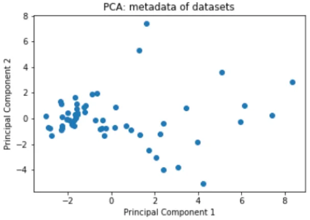
such as text classification, spam identification, breast cancer detection, and credit approval, Table C.1. Scikit-learns ‘fetch-openml’ function was utilized for this research in order to obtain the datasets from OpenML using the dataset identification number. In order to illustrate the diversity of the datasets used in this analysis, the meta-data of each dataset was transformed into two principal components and plotted in Fig. 3.1. A list of meta-data features analyzed from each dataset can be found in the Appendix, Table B.1.
Figure 3.1: Meta-data of each dataset was transformed into two principal components to show variance and diversity between each dataset used in this analysis
3.1.2
Preprocessing of data
Preprocessing is a data mining technique in which raw data is transformed in order to prepare it for a followup process – for instance, a classifier. Basic preprocessing steps include normalization, encoding, sampling, cleaning, feature extraction, and feature selection.
Minimal preprocessing on the data was performed because many algorithms in Scikit-learn require certain cleaning steps in order to run the algorithms [20]. This includes an encoder on categorical data, label encoder on labeled target columns, standard scaler on numerical data, and simple imputer for missing values. The simple imputer selected the most frequent response in the column for categorical features and the mean of the column values for numerical features. The following paragraphs will explain each preprocessing step in detail and the reasoning for
including each of these steps.
According to the Scikit-learn manual, Scikit-learn algorithms assume data is in the format of a Numpy array and cannot process categorical variables [20]. Thus, Scikit-learn machine learning algorithms require inputs variables to be numerical and cannot operate on categorical or labeled data. Moreover, some Scikit-learn algorithms, such as decision trees, cannot handle missing values; thus, it is required to impute the missing values in the input dataset.
The encoder converts the unique categorical values in the features to numerical integer values [20]. Similarly, the label encoder converts the non-numerical labels, or target columns, from 0 to the number of classes. Scaling of numeric columns in a dataset to center around zero prevents high magnitude features from dominating smaller features [20]. Scaling results in features having relatively the same orders of magnitude. Single Vector Machine, K-nearest neighbors, logistic regression, and Principal Component Analysis (PCA) are especially affected by non-scaled features since they utilize the euclidean distance in order to classify a data point [20].
3.1.3
Meta-features
We can describe datasets by extracting simple statistical properties, also known as meta-features. In this work, we will use the 49 meta-features described in Table B.1 in order to predict the expected optimization over defaults for each optimization techniques and analyze the performance of different algorithms and optimization techniques. Since the basis of this section of this research relies on capturing meta-features, we will exploit an extensive amount of qualities. This meta-feature analysis ranges from standard qualities, such as the number of instances or classes, to more advanced analyses using Principal Component Analysis (PCA) and landmark analysis. Landmarking measures the performance of the dataset on basic learning algorithms such as Linear Discriminant Analysis, Naive Bayes, and Decision Trees [16]. The performance of each algorithm can be used to characterize problem difficulty [22]. It is often challenging to
choose meta-features to describe a dataset. Therefore the meta-features chosen in this work will be building off of those in the Auto-Sklearn paper in order to keep consistency between different works [5].
3.1.4
Algorithms
Ten different classification methods were analyzed in this research, a list of the classifica-tion algorithms used can be found in the Appendix, Table A.1. The algorithms chosen include support vector machines, nearest neighbors, naive bayes, decision trees, and ensemble methods [20]. Generally speaking, the nearest neighbors algorithm is a simple classifier that assigns data points to a class based on the nearest neighbors to that point with the closest feature vector. These methods are typically less effective in high dimensional spaces because as the number of features increases, the number of training samples needed grows exponentially. Naive bayes classification methods are also relatively simple as they assume conditional independence between every pair of features. With this assumption, these algorithms estimate probability distributions from the Maximum A Posteriori (MAP). Although these methods are commonly used for their computational speed, they are known to lack accuracy/precision due to their ”naive” simplicity [20]. We considered the Gaussian and Bernoulli Naive Bayes variants in this research, in which the assumption for the probability distribution is Gaussian and Bernoulli respectively. Decision trees predict the value of the targets by learning a set of simple decision rules for different sets of data. Ensemble methods combine different estimators by either averaging the predictions, as seen in Bagging classifier, or boosting where base estimators are built sequentially, as seen in Gradient Boosting classifier. Support Vector machines model the optimal classification hyper-plane while maximizing the gap between categories. More information about each Scikit-learn algorithm used can be found on the main Scikit-learn user guide [20].
3.1.5
Hyper-parameter search spaces
The hyper-parameter search space refers to the mapping of the model hyper-parameters into a format that the optimization technique can recognize. The hyper-parameters are divided into the following types: integer, boolean, constant, enumeration, choice/conditions, and union. Boolean and enumerations are mapped as categorical hyper-parameters in which the search space consists of either True or False in the case of boolean values or a list of possible categorical values in the case of enumerations. Values which only have a singular value will be mapped as Constant hyper-parameters as they are not meant to change. Integer values will be set with an upper bound and a lower bound for the optimizer to search through. Union values refer to when a value can be multiple types, for instance, float and string values. Choice value refers to situations when there is a dependence between parameters. For instance, in support vector machines, the hyper-parameter ‘coef0’ is only significant when the hyper-parameter ‘kernel’ has the value ‘poly’ or ‘sigmoid’ [20]. In other words, conditions are applied in situations where a parameter is only activated when another hyper-parameter holds a certain value in order to minimize any unnecessary optimization. In the case of SMAC and BOHB optimization, default values will be provided for all hyper-parameters. The hyper-parameter search for these optimization techniques will start from these default values. All of the hyper-parameter configurations spaces are automatically wrapped utilizing the D3M core package as well as custom logic designed to map any primitive to the optimization hyper-parameter space. Both union and choice situations are handled internally and will ensure that no unnecessary or invalid choices are being made and sent to be evaluated. All hyper-parameter spaces including the ranges, defaults, and types can be found in the Appendix, Table A.1
3.2
Optimization Methods
The hyper-parameters of a model are usually set manually, but several methods exist to automatically selected the best values. The most popular methods of doing this are Grid Search and Random Search. Grid Search consists of setting up a grid of the hyper-parameter space and automatically looping through all combinations. Random Search, on the other hand, searches through random values within the given search space. However, these techniques are brute force methods that are inefficient and in some cases, even impractical for large datasets or large hyper-parameter spaces [27]. Grid Search, in particular, searches the entire hyper-hyper-parameter search space, and thus, it wastes resources because it explores over unimportant search spaces [27]. Both of these approaches are sub-optimal as they are not able to make use of past evaluations in order to continue evaluations on only optimal values. In contrast, Bayesian hyper-parameter optimization consists of building a model that predicts algorithm performance and uses that model in order to select the next promising hyper-parameters to evaluate [23]. Specifically, Bayesian optimization keeps past observations to build and update a probabilistic model that maps hyper-parameters to an evaluation probability score:
P(score|hyper parameter set) (3.1)
This model guides the optimal hyper-parameter search, but there are many different ways that this model can be generated. The following methods for generating the probabilistic model and optimization technique were analyzed in this paper: SMAC, Hyperopt, and BOHB.
3.2.1
SMAC
Sequential Model-based Algorithm Configuration (SMAC) is a Bayesian Optimization method which utilizes a random forest of regression trees to construct the probabilistic model [8]. The next points which are considered for evaluation are sampled from the region of greatest
expected improvement by the random forest and hence, are able to use observed hyper-parameter settings in order to explore new regions.
3.2.2
Hyperopt
Hyperopt uses a Tree Parzen Estimator(TPE) where two separate distributions are used in order to construct the optimization model [1]. These two distributions are divided based on hyper-parameter configuration results being above or below a certain threshold specified by the user. In this way, TPE is able to build the posterior distribution by selecting samples from the probability distribution of the hyper-parameters which performed above a certain threshold, or ‘good’ hyper-parameter sets. In other words, Hyperopt finds the next optimal set by reducing the ratio between the ‘good’ and ‘bad’ distributions. Hyperopt also balances between exploration and exploitation by incorporating random search in its optimization process. Thus, the optimizer is not limited to sampling only from the maximum expected improvement, or the hyper-parameter settings that the optimization model predicts will yield the best results.
3.2.3
BOHB
Bayesian optimization with Hyperband (BOHB) evaluates approximations of the prob-abilistic function on smaller budgets in order to get rid of sub-optimal configurations [4]. In other words, early investigations of the hyper-parameter search space will often yield undesirable scores as the optimizer builds the posterior distribution to determine future configurations. The underlying logic for BOHB is to utilize smaller budgets such that the entire budget is not spent rediscovering unfavorable configurations. Some examples of variables that can be budgeted include: number of iterations, number of epochs, time, and size of the dataset. In this research, budgeting was performed on a percentage of dataset points, starting from 10% of the dataset until the entire dataset was evaluated. Each iteration of BOHB consists of 100 workers that evaluate
an increasing amount of the budget until the entire budget is evaluated. Due to this budgeting structure, in this research, one iteration of BOHB is considered to be the highest score achieved when utilizing the full dataset. In this way, we are able to compare each of the optimization techniques on a per iteration level since all of the iterations represent the evaluation of the entire dataset.
There are many different implementations of Bayesian optimization with Hyperband (BOHB). According to Section B of the Supplementary material of [4], the employment of BOHB in [26] may result in weaker performance because a new model is built anew for every evaluation run, or Successive Halving in which the worst-performing half of target configuration sets are discarded [4]. Although [7] has a similar implementation of BOHB to [4], the use of the Gaussian function to model the performance might lead to weaker performance due to poor extrapolation [4]. Because of these reasons, the BOHB algorithm by [4] was analyzed in this paper and plugged into the D3M program.
3.2.4
Excluded techniques
The purpose of the following research is to give an insight into current hyper-parameter optimization techniques and time constraints. Hence, Spearmint was excluded from this list due to the repository and project inactivity.
In this research, the hyper-parameter search algorithms were run sequentially because one of them, Hyperopt, did not have parallelism enabled. Thus, it would otherwise be difficult to evaluate each unique optimization technique in parallel mode as the performance of the learning was not central problem at hand; instead this work focuses on the search effectiveness.
3.2.5
Performance Measure
To measure the performance of hyper-parameter tuned models on classification problems, optimizers were set to reduce the error in the accuracy; this is also known as the loss. The loss is a value which indicates the performance of how well or bad a model predicted. For each iteration, the scores over five cross-validation folds were averaged in order to reduce over-fitting or under-fitting. High values for the loss function indicate a bad predictor as the sum of errors on the training dataset is large. Ideally, we expect that the optimizers would observe lower loss values as the iterations increase.
3.3
Automation
In the following section, automation for this experimental experiment is described in detail. This includes automatically collecting data on an iteration level for all tuners, algorithms, and datasets as well as capturing meta-data for each dataset. The tuner plug-ins into the D3M program are also described further below. Finally, the model for prediction of optimization improvement over defaults is explained and outlined.
3.3.1
Analysis setup
Each dataset was run for 400 iterations for the tree primitives since they tended to run for relatively longer times (i.e. random forest). Primitives that were relatively faster (i.e. Gradient Boosting) were run for 600 iterations. At every iteration, the evaluated hyper-parameter settings and its associated loss were recorded for each optimizer. Moreover, the time for each iteration as well as the cumulative time until that point was noted and stored in individual files. A test set was held out to test the final optimal configuration with an unseen portion of the dataset, and those accuracy scores were reported. These experiments were run on two Ubuntu 32 core machines. All of these data files were finally congregated into one larger data frame in order to do the graphical
analysis seen in Chapter 4.
3.3.2
Auto-ML setup
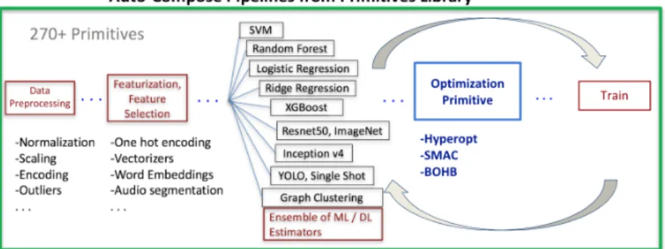
A plug-in for parameter tuning was constructed in order to easily integrate hyper-parameter optimization into the D3M program pipeline. Given any primitive with defined hyper-parameters in the D3M space, a fit method, and produce method, the plug-in automatically maps the hyper-parameters into the search space of the desired optimizer. Researchers in the D3M program can set the loss function for every optimizer, the cross-validation folds, and various resource configurations for each optimizer. This is particularly advantageous as the settings for the tuner can easily be set, and hyper-parameter optimization within the pipeline can continue seamlessly with relatively little additional effort from the user. Figure 3.2 illustrates a diagram of the optimization plug-in.
Figure 3.2: Diagram of optimization plug-in with the auto-composition pipeline framework of D3M
3.3.3
Meta-data
The meta-data discussed in this paper and described in Table B.1 in the Appendix are au-tomatically calculated from the data. After the meta-features for each dataset were calculated, the information was used to predict the optimization improvement over defaults for each optimization technique.
3.3.4
Prediction of optimization improvement over defaults
In order to construct a model for prediction of optimization improvement over defaults, a considerable amount of preprocessing of the collected data was needed. Meta-features that did not apply to certain datasets were filled in with extremely negative numbers in order to remove missing values. Algorithm names were one hot encoded such that the machine learning model would be able to interpret the column. For this research, the XGBoost regression algorithm was selected to learn the optimization improvement over defaults using the data collected across all datasets and algorithms for each tuner in addition to the meta-data for each dataset [2]. Only features with high feature importance were retained, less significant features were removed from the input dataset. A different model was trained for each unique tuner. Accuracy scores on the test dataset and features importance for each model were recorded.
Chapter 4
Results and Discussion
4.0.1
Hyper-parameter search space
Data collected from the hyper-parameter optimization runs were analyzed using various plots. Analysis plots of the examined hyper-parameter search spaces can provide insight into both the algorithmic hyper-parameters and the efficiency of the optimization method.
4.0.2
Exploring the selection of categorical values
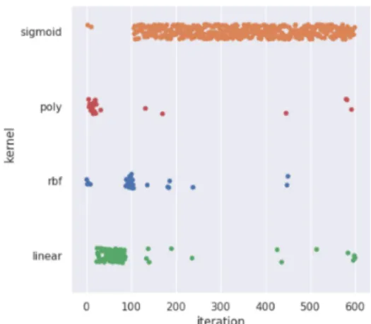
For categorical hyper-parameters, the evolutionary search over iterations provides insight on how the model searches for the optimal hyper-parameter values over time. In Figure 4.1, the Support Vector Machine (SVM) was run on the multi-class arrhythmia dataset (5) [25], and the hyper-parameters were optimized through Hyperopt, SMAC, and BOHB. Figure 4.1 shows the ‘kernel’ type value the optimizers selected for evaluation over each iteration. In all figures, one choice dominated the search space, but not all optimizers had the same value dominating the search. We see that Hyperopt and SMAC continuously selected ‘sigmoid’, whereas BOHB over-selected ‘poly’ in two separate runs, Figures 4.1 (c)(d). A rerun of SMAC with a different seed showed a graph more similar to Figure 4.1 (d). Categorical hyper-parameter values typically
Hyperopt SMAC BOHB(1) BOHB(2)
180 210 687 737
Table 4.1: Run times (in seconds) for each optimizer on the arrhythmia dataset correlating to Figure 4.1
have a dominating selection of a single value, but it might not be the same every time due to randomness in Bayesian optimization. However, it is interesting to note that there is more continuous searching over other possible values for ‘kernel’ in Hyperopt, Figure 4.1(a), than in BOHB or SMAC, Figures 4.1(b)(d). This seemed to be the case throughout all runs of categorical hyper-parameters. This exploration pattern throughout all iterations can probably be explained by the random search component in the Hyperopt tuner. We also note that BOHB has more exploration in earlier iterations as BOHB behaves more randomly in early iterations until enough data is collected.
In most cases, the over selected hyper-parameter becomes the final value selected for the ”most optimal” hyper-parameter combination after 600 runs. Despite the different choices in this hyper-parameter, all of these runs (SVM on arrhythmia dataset) resulted in similar accuracy scores ranging between 70% - 73% for all best hyper-parameter configurations selected on the test dataset from the holdout set. The time to complete the 600 iterations for SVM on the arrhythmia dataset varied between optimizers as Hyperopt and SMAC took significantly less time to complete when compared to BOHB. According to the OpenML website, there are 3,345 unique runs on the arrhythmia dataset with the highest accuracy score of 77% obtained using the Scikit-learn random forest pipeline [25]. Learning run-times for these methods are summarized in Table 4.1.
4.0.3
Exploring the selection of extreme continuous values
For certain hyper-parameters that set a min or max bound, such as values ‘min samples leaf’ or ‘max features’, we expect to see the value distributions to be skewed towards one direction or another. We expect this because the optimizer should gradually see improvement in the loss value
(a) Hyperopt: ‘kernel’ search over 600 iter (b) SMAC: ‘kernel’ search over 600 iter
(c) BOHB: ‘kernel’ search over 600 iter
RUN 1 (d) BOHB: ‘kernel’ search over 600 iter RUN 2
Figure 4.1: Evolution of the hyper-parameter ‘kernel’ for SVC on arrhythmia dataset
when using smaller numbers for ‘min samples leaf’ and using larger numbers for ‘max features’. This relationship is confirmed in Figures 4.2 (a)(b) for ‘max features’ and ‘min samples leaf‘ since both graphs are relatively skewed towards one extremity over all optimizers.
Figure 4.2 and Figure 4.3 are plots of every value selected for the specified hyper-parameters over all datasets where each unique color represents one of the three optimizers: BOHB (blue), SMAC (orange), or Hyperopt (green). Although both graphs in Figures 4.2 (a)(b) show relatively similar trends between the different optimizers, the Hyperopt distribution shows
(a) Bagging Classifier ‘max features’ (b) Extra Trees Classifier ‘min samples leaf’
(c) Extra Trees Classifier ‘min samples leaf’ over iterations for BOHB optimizer
Figure 4.2: Histogram of counts of max and min continuous values over all datasets
more uniform searching in comparison to the SMAC and BOHB optimizers. This uniform trend for Hyperopt was clear for most continuous hyper-parameters, as seen again in Figure 4.3. BOHB also shows some uniformity at a smaller frequency while SMAC displays distinct peaks throughout the spectrum of acceptable values. The patterns seen in these graphs can be explained by the unique exploration methods for each of the three optimizers. As explained in Chapter 3, Hyperopt contains a continuous exploration component, in the form of Random Search, which could explain the continuous uniformity in the search. BOHB exhibits Random Search tendencies in early iterations and becomes more refined in later iterations as it develops the posterior distribution. This trend can be more clearly seen in Figure 4.2 (c) where the development of a right skew for the hyper-parameter ‘min samples leaf’ begins after 200 iterations and becomes more defined by iteration 300. With limited exploration, SMAC mostly investigates the close neighborhoods of
the initial configurations; hence, distinct peaks appear in the search in comparison with the other optimizers.
In Figure 4.3, the selected values of ‘n estimators’ and ‘learning rate’ for the Gradient Boosting Classifier over all datasets and all iterations are plotted. As presented in Figures 4.2 (a)(b), relative to Hyperopt and BOHB, SMAC shows more distinct peaks at specific values for the hyper-parameters ‘n estimators’ and ‘learning rate’. For all three estimators, there is a relative peak of around 0.1 for the ‘learning rate’, which is expected since this hyper-parameter shrinks the contribution of each tree by this value. Typically, one would increase the number of estimators and decrease the learning rate in ensemble methods [20][18]. Although Gradient boosting classifier is robust enough to avoid over-fitting, a high enough learning rate with increasing trees could lead to over-fitting. In short, there is typically an inverse relationship between the number of estimators and the learning rate. Thus, one would expect that the distribution count of ‘n estimators’ to be closer to a uniform shape that resembles the learning rate, as seen by the Hyperopt (green) and BOHB (blue) optimizers, Figure 4.3 (b). Interestingly, the SMAC optimizer instead exhibits a distribution that is more right-skewed, as seen in Figure 4.3 (b). One possible explanation for this right skew is that the SMAC optimizer uses the default values for the hyper-parameters as the first iteration of the search and closely searches that area first. In this particular case, ‘n estimators’ was set to 100, as recommended by the Scikit-learn user guide [20]. Because SMAC tends to perform a neighborhood search rather than an exploratory search, we notice that the search for this optimizer tends to stay in the neighborhood of the initial default configuration followed by a precise search around the next best configurations. When looking from a per iteration basis, as in Figure 4.3 (c), the early iterations of SMAC start at the default configuration and slowly expand the search out towards larger ‘n estimators’ values. But a more substantial portion still remains closer to the default value of 100 and expands out to higher values at a slower rate than the other optimizers. In article [17], authors note that when implementing Auto-Sklearn, which utilizes SMAC as the underlying optimizer, they noticed a similar behavior of searching over a small
number of configurations that are close to the best so far configuration, reducing the exploration over possible values.
(a) Gradient Boosting ‘learning rate’ (b) Gradient Boosting ‘n estimators’
(c) Gradient Boosting ‘n estimators’ over iterations for SMAC optimizer
Figure 4.3: Histogram of counts of continuous values over all datasets
4.0.4
Effect of tuning and model selection
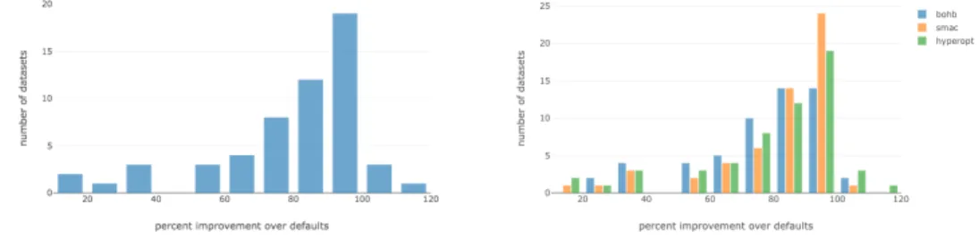
Figure 4.4 and Figure 4.5 illustrate the percent improvement over defaults for all algo-rithms evaluated. In specific, the percent improvement refers to the ratio between the smallest loss achieved through hyper-parameter optimization and the loss achieved when utilizing the default hyper-parameter values. The default values were selected based on the recommendations for the defaults as provided by the Scikit-learn user guide [20]. For each dataset, the percent improvement over defaults was calculated and aggregated into Figure 4.4 and Figure 4.5, which displays the number of datasets that achieved that percent improvement. In Figure 4.4 (a), LinearSVC shows a considerable amount of improvement over defaults for most datasets when using the Hyperopt
optimizer with the majority of datasets achieving improvements of over 60%. All three optimizers produced similar amounts of percent improvement across all datasets, as seen in Figure 4.4 (b). In addition, more models achieved percent improvement values that were over 100% when utilizing Hyperopt than any other optimizer for LinearSVC. Although SMAC did not achieve any percent improvements over 100%, we note that SMAC has the tallest peak in Figure 4.4 (b) for binned values in 90%-99%. Figure 4.5 shows that, in general, a considerable amount of improvement over defaults is achieved across all datasets and algorithms. Algorithms which had smaller search spaces, or fewer hyper-parameters to tune, achieved greater improvements over defaults than algorithms with larger search spaces. Because there are fewer values to tune, it is able to search a larger portion of the total amount of possible combinations of hyper-parameter values. Thus, more iterations would be necessary for algorithms with larger search spaces to get the same improvements as those algorithms which have smaller search spaces. In short, hyper-parameter optimization is advised for most datasets as all three optimizers achieved a large amount of improvement over defaults after only a couple hundred iterations.
(a) LinearSVC hyper-parameters opti-mized with Hyperopt
(b) LinearSVC hyper-parameters opti-mized with SMAC/BOHB/Hyperopt
Figure 4.4: Bar plot of percent improvement over default values vs. the number of datasets that achieved that value. BOHB(blue), SMAC(orange), Hyperopt(green)
(a) Hyperopt (b) SMAC
(c) BOHB
Figure 4.5: Stacked bar plot of percent improvement over default values vs. the number of datasets that achieved that value. The colors represent each algorithm evaluated.
4.0.5
Optimization times
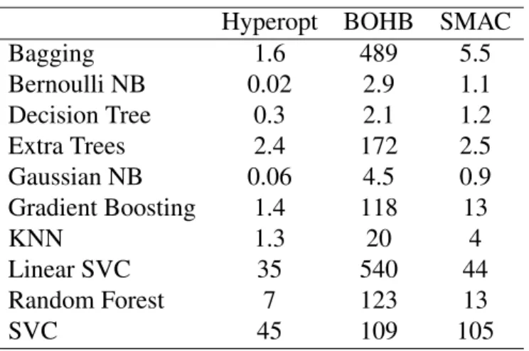
Most common users and automated machine learning systems face time constraints. Table 4.2 lists the average time in seconds to beat the loss achieved by the default values for each optimizer. Hyperopt, in general, was able to beat the default loss in a shorter amount of time than the other optimizers. There are several potential reasons for this. As explained in Chapter 3, one iteration of BOHB was considered to be when the entire budget was evaluated. BOHB budgets its resources until the full budget is used over 100 workers. Hence, it takes longer for one iteration of BOHB to complete an evaluation on the entire dataset as 100 mini-runs are performed first. As discussed in earlier results and Chapter 3, we noticed that SMAC has the least amount of exploration in comparison with the other methods described. Thus, one possible explanation for Hyperopt beating the default loss in quicker times is that it is able to randomly find better configurations while SMAC searches values around its closest neighbors first. An overall trend across all optimizers is that the amount of time to beat the default loss is considerably more for algorithms that are more complex and have more hyper-parameters to tune
and optimize. For example, support vector machines and tree algorithms take considerably more time than simpler algorithms such as Naive Bayes. Figures D.1, D.2, and D.3 in the Appendix show the average, minimum, and maximum times in seconds for all algorithms and datasets. In general, the minimum and maximum times for improving over the default values are much faster for algorithms that have fewer hyper-parameter values. Moreover, the average, minimum, and maximum times for improving over defaults were much faster for algorithms which utilized Hyperopt rather than SMAC and BOHB. Thus, the random exploration element of Hyperopt could result in faster times for the optimizer to beat default values.
Table 4.2: Avg. Time in seconds to beat default loss.
Hyperopt BOHB SMAC
Bagging 1.6 489 5.5 Bernoulli NB 0.02 2.9 1.1 Decision Tree 0.3 2.1 1.2 Extra Trees 2.4 172 2.5 Gaussian NB 0.06 4.5 0.9 Gradient Boosting 1.4 118 13 KNN 1.3 20 4 Linear SVC 35 540 44 Random Forest 7 123 13 SVC 45 109 105
4.0.6
Analysis of performance on hard and easy problems
To further analyze these optimizers, we compared the performance on the test datasets of ‘hard’ and ‘easy’ problem difficulty. We quantify problem difficulty through the landmarked meta-features that we captured and discussed earlier. To reiterate, landmarking measures the performance of basic learning algorithms on a particular dataset. Hard problems are defined as landmarked algorithms that achieved an accuracy score of less than 40%, and easy problems are accuracy scores that were greater than 95%. Specifically, the particular landmarking algorithm selected as the quantifier for problem difficulty was the simple Decision Tree. As discussed in
Chapter 3, a model was designed to predict the percent improvement for each optimizer given the dataset meta-features. A list ranking feature importance was calculated from the trained XGBoost model; this will be explored in-depth in Section 4.1. The feature ranking showed that the Decision Tree landmarking attribute held a significant amount of importance across all three tuners. Thus, it was selected as the quantifier for hard and easy problems. The accuracy scores presented in Tables 4.3, 4.4, and 4.5 utilized test data which was withheld from the training dataset.
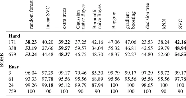
These tables contain the accuracy score from seven unique datasets which are used to analyze further how different hyper-parameter optimizers perform on very easy datasets versus very hard datasets. On the easier datasets, Hyperopt and BOHB generally performed better than SMAC for each machine learning algorithm with BOHB achieving higher accuracy scores overall. This trend does not hold for the difficult problems as no single optimizer significantly outperformed any other tuner across all algorithms. However, some algorithms seemed to achieve higher accuracy scores with certain optimizers than others. BOHB tended to outperform the other optimizers for the Extra Trees, Support Vector Machines, and Random Forest algorithm (Table 4.3). Extra Trees, Support Vector Machines, and Random Forest algorithms have only ten hyper-parameters which were optimized. Hyperopt achieved higher scores with Linear Support Vector Machines, which also have ten hyper-parameters (Table 4.4). As seen in Table 4.5, SMAC scored the highest accuracy on the more difficult problems with the Gradient Boosting algorithm. Gradient Boosting algorithm had more hyper-parameters than any other algorithm analyzed in this paper, 14 in total. In Figure 4.5, 25 datasets achieved over 75% improvement with the SMAC optimizer for the Gradient Boosting algorithm. Whereas only 16 datasets in BOHB and 17 datasets in Hyperopt achieved over 75% improvement for the Gradient Boosting algorithm. It appears from this data that SMAC outperforms the other tuners with algorithms that contain a large number of hyper-parameters.
Table 4.3: BOHB: Performance of most optimal hyper-parameter settings on ‘hard’ and ‘easy’ problems. Values in bold indicate columns which were discussed in section 4.0.6
random forest linear SVC extra trees Gaussian nai v e Bayes Bernoulli nai v e Bayes
Bagging gradient boosting decision
tree kNN SVC Hard 171 38.23 40.20 39.22 37.25 42.16 47.06 47.06 23.53 38.24 42.16 338 53.19 27.66 59.57 59.57 34.04 55.32 46.81 42.55 29.79 48.94 679 53.24 44.48 48.37 46.75 48.70 48.37 52.27 44.80 52.60 54.55 BOHB Easy 3 96.04 97.29 99.17 79.46 85.30 99.79 99.17 97.29 95.72 99.17 61 93.33 97.78 95.56 95.56 68.89 95.56 95.56 95.56 95.56 97.78 24 99.26 99.18 95.12 89.79 87.94 100 100 98.65 100 100 759 100 100 100 90 90 100 100 100 90 90
Table 4.4: Hyperopt: Performance of most optimal hyper-parameter settings on ‘hard’ and ‘easy’ problems. Values in bold indicate columns which were discussed in section 4.0.6
random forest linear SVC extra trees Gaussian nai v e Bayes Bernoulli nai v e Bayes
Bagging gradient boosting decision
tree kNN SVC Hard 171 45.10 50.98 45.10 36.27 46.08 44.12 41.18 38.24 43.14 34.31 338 44.68 48.94 53.19 55.32 40.43 51.06 42.55 46.81 55.32 38.30 679 48.05 45.78 43.18 45.45 48.05 49.03 46.43 45.13 50 53.57 Hyperopt Easy 3 93.74 97.60 93.85 80.29 87.79 99.27 99.37 93.74 96.04 99.27 61 95.56 97.78 93.33 95.56 75.56 97.78 95.56 95.56 95.56 97.78 24 97.54 98.89 95.32 90.89 88.11 100 100 94.79 100 100 759 100 95 95 80 75 100 100 100 80 90
Table 4.5: SMAC: Performance of most optimal hyper-parameter settings on ‘hard’ and ‘easy’ problems. Values in bold indicate columns which were discussed in section 4.0.6
random forest linear SVC extra trees Gaussian nai v e Bayes Bernoulli nai v e Bayes
Bagging gradient boosting decision
tree kNN SVC Hard 171 21.57 42.16 21.57 36.27 46.08 45.10 48.04 20.59 44.12 43.14 338 48.94 46.81 46.81 48.94 40.43 38.30 48.94 29.79 36.17 38.30 679 49.03 43.51 47.40 44.48 46.75 46.75 52.60 46.75 50.32 49.03 SMA C Easy 3 92.60 97.50 92.60 82.17 85.19 99.27 98.02 92.60 95.93 99.06 61 91.11 93.33 88.89 91.11 73.33 91.11 91.11 91.11 88.89 99.11 24 91.91 99.18 94.54 89.91 86.96 100 100 87.16 100 100 759 100 100 100 80 85 100 100 100 90 100
4.0.7
Performance by Dataset
For each dataset, the overall best score across all algorithms was compared for each optimizer. For this section, overall best scores across all algorithms are analyzed as this paper’s primary focus is geared towards Auto-ML systems. This is not a definitive analysis as runs should be done multiple times in order to capture randomness between runs. A more comprehensive review would be necessary for this and has already been explored in [3][28][4]. In the 59 datasets run, BOHB was the best optimizer in 8 cases, Hyperopt for 8 cases, and SMAC in 4 cases. The best optimizer which outperformed the other optimizers was defined as having a score of greater than 2% from the second-highest score. There was a significant amount of ties between different optimizers. Hyperopt and SMAC had ties in 2 cases, Hyperopt and BOHB had ties in 9 cases, BOHB and SMAC had ties in 4 cases. In 24 cases, all three optimizers had a tie on the test sets. In most cases, the optimizers performed relatively the same on the withheld test dataset. Overall, BOHB achieved the maximum score on more datasets than SMAC and Hyperopt (45 out of 59 datasets). In short, no single tuner outperformed all other tuners over all datasets.
4.0.8
Performance by Algorithm
To bulk compare performance of tuners across ten algorithms, a ranking system is used as a measure of performance. The ML algorithms are ranked by the accuracy score of each algorithm on the test dataset for each of the 59 problems. The mean performance ranking of the algorithms across all datasets is plotted in Figure 4.6. Lower rankings indicate higher accuracy scores, while higher rankings indicate lower accuracy scores. These plots show that overall ensemble-based tree algorithms are higher performing on average than naive Bayes algorithms. As explained in Chapter 3, we expected naive Bayes algorithms to rank lower due to its naive simplicity. When looking at each individual tuner, BOHB observes lower rankings for ensemble-based tree algorithms than the other two methods, Figure 4.6 (c). SMAC shows lower rankings for LinearSVC as it was the fourth-ranked algorithm in the tuner when compared with seventh-ranked (Hyperopt) and sixth-ranked (BOHB), Figure 4.6 (a).
4.1
Optimization prediction model
As shown in Section 4.0.4, hyper-parameter tuning results in improved scores over the default values in almost all cases. In earlier sections, we discussed situations in which certain tuners tended to perform better than other tuners. In order to pre-determine which tuner might perform better given a dataset and algorithm, a model was constructed to predict the percent optimization over defaults for each tuner. As discussed in Chapter 3, three different models were created for each tuner. The Correlation Coefficient for each model is as follows: SMAC (0.51), BOHB(0.54), and Hyperopt (0.56). The models yielded moderate correlation coefficients indicating that there is some sort of correlation between tuner and percent optimization expected. This could be further investigated as part of a larger effort for achieving a viable prediction model. An alternative purpose of these models is to calculate the most significant meta-features in predicting the percent optimization over defaults for each tuner. Tables 4.6, 4.7, and 4.8
summarize the results of the top eleven meta-features from the learned model. From these tables, it appears that we see some similar observations as previously seen in Section 4.0.6. In Section 4.0.6, BOHB appeared to achieve higher scores with the tree algorithms, and we observe in Table 4.7 that four tree algorithms are in the top 11 most important meta-features. We also previously discussed how Hyperopt scored higher accuracy scores with LinearSVC, which is also the ranked third in feature importance in Table 4.8.
Table 4.6: Raked meta-features for predicting percent optimization for SMAC
Rank Meta-feature
1 Minimum of the ratios of data-points in each class
2 The minimum number of unique symbols across all categorical features
3 Bagging
4 Extra Trees
5 Landmark with decision tree
6 Gradient Boosting
7 Standard Deviation of the ratios of data-points in each class
8 K Nearest Neighbors
9 Landmark with decision node learner
10 Ratio of numerical features to categorical features 11 Support Vector Machine
Table 4.7: Raked meta-features for predicting percent optimization for BOHB
Rank Meta-feature
1 Landmark with knn (n=1) 2 Number of categories
3 Maximum kurtosis value on numerical features 4 Landmark with decision tree
5 Bernoulli NB 6 Extra Trees 7 Random Forest 8 Decision Tree 9 Number of instances 10 Gaussian NB 11 Gradient Boosting
Table 4.8: Raked meta-features for predicting percent optimization for Hyperopt
Rank Meta-feature
1 Landmark decision tree
2 The ratio of number of features to the number of data points
3 Linear SVC 4 Gaussian NB 5 Bernoulli NB 6 Gradient Boosting 7 Bagging 8 Landmark with knn (n=1) 9 K Nearest Neighbors
10 The sum of unique symbols for each categorical feature 11 Number of instances
(a) SMAC: Average ranking of the ML al-gorithms
(b) Hyperopt: Average ranking of the ML algorithms
(c) BOHB: Average ranking of the ML al-gorithms
Chapter 5
Conclusion
There are many different methods available for hyper-parameter optimization, such as BOHB, SMAC, and Hyperopt. In most Auto-ML systems and common-user pipelines, there is only one type of hyper-parameter optimization technique utilized. However, each unique optimization technique has its own advantages and disadvantages. For instance, Hyperopt has a large amount of random search implemented throughout the search, whereas SMAC fine-tunes in the neighboring regions. Thus, understanding the search method and how these optimizers produced the values that were deemed optimal is very insightful for ways to improve and make searches more efficient. For instance, in the case of categorical values, it is useful to note that the ‘dominant’ value is usually the value that is part of the final incumbent configuration. An in-depth analysis of the search of a hyper-parameter optimizer also gives clues on the trade-off between exploration and exploitation. For a shallow search over a large number of algorithms, an Auto-ML system may choose an optimizer such as Hyperopt because it implements a large amount of Random Search throughout the optimization. Moreover, such an optimizer could potentially be useful as one can achieve desirable results much quicker than the other two optimization methods (Table 4.2). The SMAC optimizer, on the other hand, has a larger focus on exploitation rather than exploration and searches the immediate neighboring space and expands out over more iterations
(Figure 4.3 (c)). BOHB is a happy medium between these two methods as it exhibits random search tendencies in early iterations and focused search in later iterations, Figure 4.1 (d). In this analysis, BOHB performed very well over most algorithms and datasets and achieved the highest test score in the most problems. However, no one optimization technique outperformed the others in all datasets.
Because of the varying advantages of different optimization, our research suggests that the selection of a hyper-parameter tuner should be based on the design of the Auto-ML system for constructing pipelines. Thus, for a large research project, such as DARPA’s Data-driven discovery program, it is advantageous to create a plug-in optimization method for any Auto-ML system. There is a large amount of continuous research for making hyper-parameter optimization more effective and efficient. Thus, this design is particularly advantageous as new optimization methods can easily be plugged into existing Auto-ML systems. Moreover, one can implement different optimization techniques depending on the structure of their search method. For instance, a system can implement Hyperopt for generalized searches which takes advantage of exploration, and then follow with fine-tuning with the SMAC optimizer. Systems such as Auto-Sklearn and Hyperopt-Sklearn are incompatible with the DARPA D3M system as users are limited to a small number of algorithms whose search spaces are hard-coded in the software [5][9]. The implementation presented in this system automatically wraps any algorithm in the program which follows the D3M convention. It also handles difficult cases such as Union and Choice hyper-parameters. This is particularly important as the implementation of conditions for choice cases can significantly reduce the search space. In short, each Auto-ML system has the flexibility to use different optimizers based on their search preference, the flexibility to use algorithms that are not in the Scikit-learn library, selection of loss function, and easy customization of optimizer settings.
Future research could include reruns of the experiments and analyzing more optimization techniques other than the three presented in this paper, such as genetic optimizers. This paper
focused on comparing tuners over classification problems. Moreover, it would be interesting to see how other algorithms, datasets, and problem types (i.e. regressions, graph problems, deep nets) respond to these hyper-parameter tuning techniques.
We hope that with this work, users are more informed regarding the selection of hyper-parameter tuning systems and effectively identifying which tuner would be more appropriate for their specific application. In addition, the aggregated metadata may help in identifying possible areas of improvement for each of these optimization techniques based on the analysis presented in this work.
Appendix A
Hyper-parameters
Table A.1: Hyper-parameters tuned for each ML algorithm. λrefers to the total number of
hyper-parameters that were tuned.
Algorithm λλλ Type Parameter Default Range
Support Vector Machine
9 Bounded(float) C 1 [0.1, 100]
Choice kernel ‘rbf’ [‘linear’, ‘poly’, ‘rbf’,
‘sigmoid’]
Bounded(int) degree 3 [0, 6]
Union(float, const)
gamma ‘auto’ [0, 10][‘auto’]
Enumeration decision function shape ‘ovr’ [‘ovr’, ‘ovo’]
Bounded(float) tol 0.001 [0.001, 0.1]
Union(str, const)
class weight None [‘balanced’, None]
Table A.1: continued from previous page
Algorithm λλλ Type Parameter Default Range
Bool probability False [True, False]
Bool shrinking True [True, False]
LinearSVC 10 Enumeration penalty ‘l2’ [‘l1’, ‘l2’]
Enumeration loss ‘squared
hinge’
[‘squaredhinge’, ‘hinge’]
Bool dual True [True, False]
Bounded(float) tol 0.0001 [0.0001, 0.1]
Bounded(float) C 1 [0.1, 100]
Enumeration multi class ‘ovr’ [‘crammersinger’,‘ovr’]
Bool fit intercept True [True, False]
Bounded(float) intercept scaling 1 [1, 10]
Union(str, const)
class weight None [‘balanced’, None]
Bounded(int) max iter 1000 [0, 4000]
Extra Trees 10 Bounded(int) n estimators 100 [1, 1500]
Enumeration criterion ‘gini’ [‘entropy’, ‘gini’]
Union(int, const)
max depth None [0, 15][None]
Bounded(float) min samples split 0.25 [0, 1]
Bounded(float) min samples leaf 0.25 [0, 0.5]
Bounded(float) min weight fraction leaf 0 [0, 0.5]
Table A.1: continued from previous page
Algorithm λλλ Type Parameter Default Range
Union(str, const, float)
max features auto [‘auto’,‘sqrt’,‘log2’]
[None] [0,1]
Bounded(float) min impurity decrease 0 [0, 0.4]
Bool bootstrap False [True, False]
Union(str, const)
class weight None [‘balanced’, None]
Random Forest
10 Bounded(int) n estimators 100 [1, 1500]
Enumeration criterion ‘gini’ [‘entropy’, ‘gini’]
Union(int, const)
max depth None [1, 15][None]
Bounded(float) min samples split 0.25 [0, 1]
Bounded(float) min samples leaf 0.25 [0, 0.5]
Bounded(float) min weight fraction leaf 0 [0, 0.5] Union(str,
const, float)
max features auto [‘auto’,‘sqrt’,‘log2’]
[None] [0,1]
Bounded(float) min impurity decrease 0 [0, 0.4]
Bool bootstrap True [True, False]
Union(str, const)
class weight None [‘balanced’, None]
Decision Tree
10 Enumeration splitter ‘best’ [‘best’, ‘random’]
Table A.1: continued from previous page
Algorithm λλλ Type Parameter Default Range
Enumeration criterion ‘gini’ [‘entropy’, ‘gini’]
Union(int, const)
max depth None [1, 15][None]
Bounded(float) min samples split 0.25 [0, 1]
Bounded(float) min samples leaf 0.25 [0, 0.5]
Bounded(float) min weight fraction leaf 0 [0, 0.5] Union(str,
const, float)
max features None [‘auto’,‘sqrt’,‘log2’]
[None] [0,1]
Bounded(float) min impurity decrease 0 [0, 0.4]
Bool presort False [True, False]
Union(str, const)
class weight None [‘balanced’, None]
Gradient Boosting
14 Enumeration loss ‘deviance’ [‘deviance’,
‘exponen-tial’]
Bounded(float) learning rate 0.00001 [0, 1]
Bounded(int) n estimators 100 [1, 1500]
Bounded(int) max depth 3 [1, 15]
Enumeration criterion ‘friedman
mse’
[‘friedmanmse’, ‘mse’, ‘mae’]
Bounded(float) min samples split 0.25 [0, 1]
Bounded(float) min samples leaf 0.25 [0, 0.5]
Bounded(float) min weight fraction leaf 0 [0, 0.5]